Modeling Object Pursuit for 3D Interactive Tasks in Virtual Reality Lei Liu∗
Robert van Liere† CWI, Amsterdam, NL
A BSTRACT Models of interaction tasks are quantitative descriptions of relationships between human temporal performance and the spatial characteristics of the interactive tasks. Examples include Fitts’ law for modeling the pointing task and Accot and Zhai’s steering law for the path steering task, etc. Models can be used as guidelines to design efficient user interfaces and quantitatively evaluate interaction techniques and input devices. In this paper, we introduce a 3D object pursuit interaction task, in which users are required to continuously track a moving target in a virtual environment. The entire movement of the task is broken into a tracking phase and a correction phase. For each phase, we propose a model that has been verified by two experiments. As the experimental results show, the time for the tracking phase is fixed once a task has been established, while the time for the correction phase usually varies according to some characteristics of the task. It can be modeled as a function of path length, target width and the velocity with which the target moves. The proposed model can be used to quantitatively evaluate the efficiency of user interfaces that involve the interaction with moving objects. Index Terms: H5.1 [Information Interfaces and Presentation]: Multimedia Information Systems—Artificial, augmented, and virtual realities; H5.2 [Information Interfaces and Presentation]: User Interfaces—Ergonomics, Theory and methods 1
I NTRODUCTION
In physiology, pursuit is defined as the action of the eye in following a moving object. In this paper, we introduce the term to describe an interaction task, in which users are required to continuously track a 3D moving object with a tracker held in their hands in a virtual environment. Object pursuit tasks can be found extensively in gaming, video surveillance system, air traffic control system, etc. A shooting game with moving targets, for example, is a typical pursuit task. As with pointing and path steering, object pursuit can be considered to be a primitive but unique interaction task. One major characteristic it differs from pointing and steering tasks is that in an object pursuit task, subjects interact with a non-stationary target which is usually kept stationary in a pointing or a path steering task. In human computer interaction, modeling is the approach to quantify interaction tasks. Widely used and well known examples include Fitts’ law [7] for modeling pointing task and Accot and Zhai’s steering law [1] for path steering task, etc. Models formally describe quantitative relationships between human temporal performance and the spatial characteristics of an interactive task. Interaction models have guided user interface designers in designing efficient user interfaces [20, 16]. They also provide a quantitative approach to evaluate the efficiency and performance between e.g. input devices [17, 2] or interaction techniques [15], etc. ∗ e-mail: † e-mail:
[email protected] [email protected]
The goal of this paper is to derive a model for the 3D object pursuit interactive task. The complete object pursuit movement is divided into a tracking phase and a correction phase. For each phase, we propose a model to describe the temporal information. The time for the tracking phase is fixed once a task has been established, while the time for the correction phase usually varies with the characteristics of the task. The correction time can be modeled as a function of the size and velocity of the target and the path length crossed by the target. The model has been verified by two experiments with repeated measures design. As indicated by the experimental results, the growth of the velocity with which the target moves usually results in longer correction time, but shorter tracking time. Therefore, the selection of the target velocity is important on reducing the total time (tracking time + correction time) of an object pursuit task. By analyzing the proposed model, we manage to derive a velocity, with which the total movement time reaches its minimum. This velocity, described as a function of path length and target width, can be used as a guide in designing user interfaces with moving targets. Furthermore, there are several aspects that we can learn from modeling the object pursuit task for a general interaction task. The way that the influence of path length and target width combines in object pursuit tasks very much resembles the way how it affects pointing and path steering tasks. This fact may be interpreted as evidence of such combination in modeling a general interactive task. In addition, the model also reveals that at least one time-related factor, besides spatial factors, is required to model an interactive task that involves a non-stationary target. The time-related factor, e.g. the target velocity in the object pursuit task, plays such an important part that it may even become an overwhelming factor in affecting users’ performance time. We suggest that both time and space-related factors should be taken into account when modeling an interaction task with moving targets. The main contributions of this work focus on the following points: • We propose to analyze an object pursuit task in such a way that the complete movement should be broken into a tracking phase and a correction phase (see Section 3.3 for details); • We point out that the time for the tracking phase is fixed if the task has been established. It can be described by Ttracking =
L v
(1)
when the target moves a distance L with a uniform velocity v (see Section 4); • We propose a model for the time of the correction phase, which has been experimentally verified. It has the following form (see Section 4.2.3): log(Tcorrection ) = a + b
L +c v W
(2)
where a, b and c are the empirically determined constants, and L, W and v are the path length, target width and target velocity.
• We manage to derive an optimal target velocity with which the total time (Ttracking + Tcorrection ) can be minimized. This velocity can be expressed with path length and target width (see Section 5). 2 R ELATED W ORK 2.1 Pursuit Task Pursuit is one of the important human skills that have been used, for example, to differentiate normal subjects from psychiatric patients [12, 8, 9] or to qualify a pilot [11, 19]. Given the parts of the human body that are used, pursuit can be categorized into eye movement [13, 3], locomotion [4], manual tasks [21], etc. It has been extensively studied in the discipline of psychology, but has never been systematically investigated as an interaction task in human computer interaction. In this paper, we use the term to describe an interaction task that requires subjects to manually steer an input stylus in pursuit of a 3D target that moves with uniform velocity in a virtual environment. 2.2 Modeling Interaction Task In human-computer interaction, there are quite a few wellformalized and accepted quantitative models that can be used as tools to compare the efficiency between interaction techniques or input devices. One of the best known model Fitts’ law, proposed by Paul Fitts in 1954 [7], has a long history and a widely applied scope [22, 6, 17]. It predicts that the time required to rapidly move to a target is a function of the distance to and the size of the target. Fitts’ law has been used to model the act of pointing in both the physical world [5] and the virtual environment [10, 24]. One common formulation of the law is as follows: T = a + b ID = a + b log2 (
L + 1) W
It is important to note that the models mentioned above all describe the temporal information with the spatial characteristics of the tasks. In this paper, we use a similar way to propose a model for 3D object pursuit task. 3
E XPERIMENT
3.1 Apparatus and Environment The experiment was performed in a desktop virtual environment as shown in Figure 1. The specific apparatus includes: • • • •
a desktop PC equipped with high end GPU, a Samsung 67-inch 3D-capable LED DLP HDTV, a pair of Crystal Eyes stereoscopic LCD glasses, a Polhemus FASTRAK connected with one 6DOF stylus tracker (sampling @ 120Hz), • a 6DOF ultrasound Logitech head tracker (working @ 60Hz). During the experiment, the resolution of the Display was set to 1920 × 1080 @ 120Hz. The end-to-end latency was measured to be approximately 80ms with the method proposed by Steed [23].
(3)
where a and b are experimentally determined constants, L is the distance to the target, and W is the target width. The term log2 (L/W + 1) is referred to as the index of difficulty (ID) of a pointing task. It was not until a few decades later that Accot and Zhai derived the steering law [1, 25] from Fitts’ law for path steering tasks. The idea of the steering law assumes that a path steering task is composed of an infinitive number of goal crossing tasks, each of which could be separately modeled by Fitts’ law. If the path width varies with the path, the generic steering law can be expressed in the following formula: ∫
TC = a + b ID = a + b
ds C W (s)
(4)
where a and b are empirically determined constants, C is a curved path, s is the elementary path length along C and W (s) is the path width at path length s. If the path width keeps fixed, the steering law can be rewritten as: TC = a + b
L W
(5)
with L and W representing the length and width of the path, respectively. However, as Liu et al. [14] questioned, it is counterintuitive to describe the steering time only as a function of path length and width. They proposed to involve other factors to the steering law as shown below: log(T ) = a + b ID = a + b(log
L + cρ ) W
(6)
where ID is redefined as log(L/W ) + cρ , introducing the influence of curvature ρ of the steering path, together with length L and width W.
Figure 1: The experimental environment: a head tracked stereo display and a 6DOF input stylus. Several depth cues were created during the experiment, including the stereoscopic viewing, head tracking, head lighting, wire-frame box and the chessboard pattern floor.
The experiment was set up in a non-colocated environment with a distance of 0.65m between the visual and motor space (see Figure 2). The control and display ratio was always kept 1. The origin of the visual space was set to 0.4m in front of the display and 0.6m above the desktop, while that of the motor space was 0.3m ahead of the subject and 0.3m above the desktop. Subjects were seated 1.35m away from the display and were required not to rest their arms on the table. 3.2 Subject Twenty right-handed subjects voluntarily participated in the experiment. There were six females and fourteen males, aged 24 to 35. Five of them were invited to perform a pilot study, while the remaining fifteen subjects were instructed to take part in the following main experiment. The experienced and non-experienced subjects were kept in a ratio of 2:3 in both pilot study and main experiment.
stereoscopic glasses
3.4 Procedure
1.35 0.4 0.65
head tracker
0.72 0.4 0.4 0.6
0.3
motor space
visual space
display
Figure 2: The experimental setup [14] (units: meter): Motor and visual space were not co-located and C-D ratio=1.
3.3 Task The experiment was designed to examine the object pursuit tasks performed by the subjects. For this, subjects were required to hold an input stylus, represented as a 3D pen in the virtual environment, with their dominant hands to trace a target (3D ball) moving in the visual space. To enhance the visual feedback, 3D coordinate axes were attached to the tip of the pen. The space in which the 3D ball moved were encapsulated in a 0.72×0.4×0.4m3 (length × height × depth) sized wire-frame box, whose floor was covered with a chessboard pattern (See Figure 1 and 2). In the initial phase, subjects were shown a stationary target ball and both the ball and the axes attached to the pen were colored red. The target ball started to move with a uniform velocity, once the tip of the pen, i.e. the origin of the 3D axes was inside the target ball (see Figure 3, right). Meanwhile, the ball and the axes turned to green. Subjects were asked to track the moving target by keeping the tip of the pen within the ball as possible as they could. If they failed, the moving target stopped, making the axes and the ball red again (see Figure 3, left). Subjects had to correct this movement by steering the pen back to the ball and resuming the tracking where they left off. A trial started when the target ball left the initial position and proceeded until the target ball moved to a predefined destination that was not known to the subjects in advance. Consequently, subjects were shown the number of trials left on the screen.
A pilot study was carried out before the main experiment with the purpose of acquiring a proper model and parameter setting for the upcoming main experiment. The design of the pilot study was different from that of the main experiment in a way that it distinguished the effect of velocity of the moving target from that of target width and path length, examining the effect of only a minimum number of independent variables at a time. Therefore, the study was split into four independent pilot studies. In pilot study 1 and 2 where velocity was fixed, we examined linear and circular paths respectively with 2 target widths and 3 path lengths, while in pilot study 3 and 4 where path length and target width were kept constant, linear and circular paths were studied with 10 velocities. As a result, two sizes for the target ball, three lengths for path and five constant velocities of the target ball were selected for the main experiment. We have conducted two main experiments of repeated measures design, in which two types of paths of the moving target were applied. The target ball always made a uniform motion on a straight path (see Figure 3.4, left) in experiment 1, while it moved along a segment of a circular path (see Figure 3.4, right) with a constant velocity in experiment 2. The radius of the target ball was set to 0.015m and 0.02m, constraining the movement of the pen to 0.03m and 0.04m in amplitude. We chose 0.24m, 0.30m and 0.36m as the path length so that completing an object pursuit task only required the extension of the arm, keeping the body relatively still. The velocity of the moving target, including 0.10, 0.15, 0.20, 0.25, 0.30m/s, was tested to be suitable to track for both nonexperienced and experienced subjects. Each combination of the above parameters was repeated three times, resulting in 2×3×5×3 (target size× path length×motion velocity×repeats) trials in each experiment and a total number of 180 trials for a subject. To compensate the practice effect, trials were presented in a random order that differed from one subject to another. Subjects were allowed to have a break whenever they suffered from fatigue between trials. This was, however, strictly prohibited during a trial.
ρ=0
ρ=8
Figure 4: Two types of paths used in Experiment 1 (left) and 2 (right). The curvature of the path, represented by ρ , is defined as the reciprocal of the path radius. The paths were not shown to the subjects.
Target ball
4 Input stylus
3D coordinate axes
Correc!on
Tracking
Figure 3: The correction phase (left) and the tracking phase (right) for an object pursuit task.
The time when the tip of the pen was within the target ball and moved with it was defined as the tracking time, i.e. the total time when target ball remained green, while the time when the tip of the pen deviated from target ball and the subject made a correction was defined as the correction time, i.e. the total time when the target ball remained red. The time for completing an object pursuit task, i.e. the sum of the tracking time and the correction time, was defined as the total time.
R ESULT
To model the object pursuit tasks, inspired by Fitts’ law and steering law, we chose to statistically explore a relationship between the temporal information, e.g. the tracking time Ttracking , correction time Tcorrection and total time Ttotal = Ttracking + Tcorrection , and the characteristics of the tasks, e.g. the target size W , the velocity of the moving target v and the path length L crossed by the target during a trial. The tracking time, i.e. the time when the target ball moves with a constant velocity, can be described as: Ttracking =
L1 L2 Ln L + + ... + = v v v v
(7)
where Ln is the length of the n-th path segment crossed by the target ball without a correction. As can be seen, Ttracking is constant if L and v have been fixed. Different from Ttracking , modeling Tcorrection requires ANOVA and regression analysis. It is, therefore, necessary to verify if the
0.7
0.7 T distribution Normal distribution
0.6
density
density
0.5
0.4 0.3
0.3 0.2
0.1
0.1 0
2
4
0
6
1
Raw data Linear model
0.5 0 −0.5 −1 5
6
7
8
9
10
11
12
13
L/W
Figure 7: Pilot study 1: Linear regression between log(Tcorrection ) and L/W for linear paths where each asterisk represents a mean correction time of a certain L/W and the corresponding error bar is its 95% confidence interval calculated using the method in [18]. The oblique line is the model fitting onto log(Tcorrection ) using Equation 8.
0.4
0.2
0
T distribution Normal distribution
0.6
0.5
1.5
log(Tcorrection)
data is normally distributed. Figure 4 plots the associated probability density function of Tcorrection for experiment 1 and 2, correspondingly. As shown, both histograms considerably deviate from the normal distribution that fits onto the data (right-skewed). A data transformation is needed to bring the density function closer to that of a normal distribution. Our approach was to apply natural logarithmical transformation (base e) to Tcorrection . As illustrated in Figure 6, the data after transformation approximately follow a bellshaped density function. The Kolmogorov-Smirnov test shows that the null hypothesis, i.e. the transformed data have a normal distribution, can not be rejected (h = 0) at the 5% significance level in each experiment.
0
2
T
4
the goodness of the fit can be evaluated by R2 =0.9528 (close to 1). A similar plot for pilot study 2 which studies the same L/W values for circular paths is demonstrated in Figure 8. The model fits the data with R2 =0.9686.
6
T
correction
correction
2
0.6
0.7
log(T) distribution Normal distribution
0.6
0.4 0.3 0.2
0 −4
0.5
6
7
8
9
10
11
12
13
L/W
0.4 0.3
Figure 8: Pilot study 2: Linear regression between log(Tcorrection ) and L/W for circular paths.
0.2
0.1
1
−0.5 5
0.5
density
density
0.5
Raw data Linear model
0 log(T) distribution Normal distribution
0.1 −2
0
2
4
0 −4
−2
log(Tcorrection)
0
2
4
log(Tcorrection)
Figure 6: The distribution of log(Tcorrection ) in experiment 1 (left) and experiment 2 (right). The histograms represent the distribution of log(Tcorrection ), while the red curves represent the pdf of the normal distribution fitting onto the data.
4.1 Pilot Study The pilot study, prior to the main experiment, was conducted with five subjects. It aims at roughly revealing how Tcorrection could be modeled with W , L and v. Intuitively, a smaller W , a longer L or a larger v is expected to result in a longer Tcorrection . In pilot study 1 and 2, therefore, we simply hypothesize that the relationship has the following form: log(Tcorrection ) = a + b
L W
(8)
The idea above is based on the fact that the temporal characteristics of both pointing task (Equation 3) and steering task (Equation 6) could be successfully modeled by term L/W . Since the definition of L and W is quite similar in these interaction tasks, we assume that there should be some correlation between the correction time and L/W for an object pursuit task. Figure 7 illustrates how model 8 fits onto the data from linear paths. As shown, there is a strong linear relationship between log(Tcorrection ) and L/W , evidenced by the fact that the linear model passes through the 95% confidence intervals of the six means and
As the values selected above provide widespread representation, they were appointed as the values of L and W for the main experiments. In pilot study 3 and 4, we hypothesize a linear relationship between log(Tcorrection ) and v in a formula below: log(Tcorrection ) = a + b v
(9)
Figure 9 and 10 specify log(Tcorrection ) in terms of various values of v and how Equation 9 fits onto log(Tcorrection ) for linear paths and circular paths. 1.5
log(Tcorrection)
0.7
1.5
log(Tcorrection)
Figure 5: The distribution of Tcorrection in experiment 1 (left) and experiment 2 (right). The histograms represent the distribution of Tcorrection , while the red curves represent the pdf (probability density function) of the normal distribution fitting onto the data.
1
Raw data Linear model
0.5
0
−0.5 0
0.05
0.1
0.15
0.2
0.25
0.3
0.35
0.4
0.45
v
Figure 9: Pilot study 3: Linear regression between log(Tcorrection ) and v for linear paths. Asterisks represent the average log(Tcorrection ) for different values of v, while the error bars represent the associated 95% confidence intervals. The oblique line is the linear model fitting onto the data using Equation 9.
between the actual data and the result of the fit. The regression parameter estimates are shown in Table 1. The fact that the 95% confidence intervals of coefficient b does not include zero illuminates that L/W is an independent variable that significantly influence the correction time of the object pursuit tasks.
log(Tcorrection)
2 Raw data Linear model
1.5
1
Coef. a b
0.5
0 0
0.05
0.1
0.15
0.2
0.25
0.3
0.35
0.4
0.45
Value -2.287 0.245
[95% Conf. Interval] [-3.316, -1.258] [0.130, 0.360]
v
Figure 10: Pilot study 4: Linear regression between log(Tcorrection ) and v for circular paths.
It can be seen that there is a strong linear correlation between the log(Tcorrection ) and v in both linear and circular paths, evidenced by R2 =0.9410 and 0.9418, respectively. However, as reported by the subjects, a tracking task with a target moving faster than 0.35m/s is too difficult to achieve, we decided to control the velocity of the moving target below 0.35m/s. There is also a velocity threshold, as indicated in Figure 9 and 10, under which subjects find the tracking task so easy to fulfil that the correction time stays relatively constant. This threshold should fall between 0.05m/s and 0.1m/s. Therefore, we chose five proper velocities for the main experiments, including 0.10, 0.15, 0.20, 0.25, 0.30m/s.
Table 1: Experiment 1: regression parameter estimates on log(Tcorrection ) fitting onto Equation 8 for linear paths.
A similar analysis has been done for the circular paths in experiment 2 (see Figure 12). As indicted by the results of the repeated measures ANOVA (F(5,70)=20.225, p