Progress In Electromagnetics Research B, Vol. 44, 89–116, 2012
MODELING OF METASHEETS EMBEDDED IN DIELECTRIC LAYERS M. Y. Koledintseva1, * , J. Huang2 , R. E. DuBroff 1 , and B. Archambeault3 1 Missouri
J. L. Drewniak1 ,
University of Science and Technology, Rolla, MO 65409-0040,
USA 2 Nokia, 3 IBM,
San Diego, CA 92127, USA
Research Triangle Park, NC, USA
Abstract—Metasheet structures together with bulk composite dielectric layers can be used for antenna radomes, absorbers, and band gap structures. Transmission (T ) and reflection (Γ) coefficients for a plane wave incident at any angle upon a metasheet embedded in a dielectric layer are considered. These metasheets are either patch-type or an aperture-type, and they can be either singlelayered or multi-layered. To calculate T and Γ for a patch-type metasheet, a concise unified matrix approach is derived using the Generalized Sheet Transition Conditions (GSTC). The Babinet duality principle is utilized to get T and Γ for single-layered aperture-type metasheets (as complementary to the patch-type ones) at an arbitrary angle of incidence. The T-matrix approach is applied to calculate characteristics of multilayered metasheet structures containing a cascade of metasheets and dielectric slabs. In this paper, the minimum distance for neglecting higher-order evanescent mode interactions between the metasheets has been determined. Computed results based on the proposed analytical approach are compared with the full-wave numerical simulations. The analytical results are verified for satisfying the energy balance condition.
Received 9 July 2012, Accepted 11 September 2012, Scheduled 18 September 2012 * Corresponding author: Marina Y. Koledintseva (
[email protected]).
90
Koledintseva et al.
1. INTRODUCTION The development, research, and applications of metamaterials (MM), metafilms (MF), photonic bandgap (PBG) crystals, and artificial dielectric or magnetodielectric composite materials with desirable frequency responses are of an increased interest [1–5]. A metafilm, or a metasheet (MS), is the two-dimensional case of a metamaterial, and it can be either of a patch type (a dielectric film with identical metallic patches on it), or of an aperture type (conducting film with apertures, typically on a dielectric substrate). Thin planar metasheets find application over a wide range of frequencies from RF to the visual spectrum for designing antenna systems, filters, shielding enclosures, screens, and absorbers. Such structures have been studied, for example, for the development of frequency-selective surfaces (FSS) [6, 7], and for perforated film absorbers, such as CARAM (Circuit-Analog Radar Absorbing Materials) [8, 9]. FSSbased structures are used in antenna radomes [10], patch antennas [11], as well as controllable microwave absorbers [12]. Frequency characteristics of transmission (T ) and reflection (Γ) coefficients of MS with simplest patterns have been analyzed using full-wave numerical methods, especially at arbitrary angles of electromagnetic incidence [13–15], as well as analytically (see, e.g., [16– 20], and references therein). The generalized sheet transition condition (GSTC) for averaged macroscopic fields across a metafilm is proposed in [16]. GSTC relates field discontinuities to the electric and magnetic polarization densities of scatters on a metafilm. Based on the GSTC approach, the analytical formulas for T and Γ have been derived in [21], both for normal and oblique incidence. The GSTC approach is very attractive for designing metafilm shielding and filtering structures, since it substantially simplifies modeling and reduces computational resources, provided the polarizability of a desired pattern is determined in advance. A polarizability of interest may be retrieved comparatively easily either analytically or numerically, as is done in [22–26]. The formulation presented in [16] and [21] allows for treating polarizabilities only in the form of diagonal tensors, while the crosscoupling between electric and magnetic polarizabilities of metafilm elements is not taken into account. However, in many cases electric and magnetic cross-coupling cannot be neglected in principle, and the GSTC approach is not applicable to many pattern geometries. The examples of such pattern geometries are an edge-coupled split-ring resonator [27–29] and an Ω-particle used in chiral media [30]. Therefore one of the objectives of the present paper is to modify the GSTC for the case of cross-coupled electric and magnetic polarizabilities.
Progress In Electromagnetics Research B, Vol. 44, 2012
Ht
91
Kt
Figure 1. General geometry and main vectors describing interaction of a plane wave with a metasheet in cartesian coordinates. Another objective is modeling multilayered metasheet structures, which provide more degrees of freedom in engineering material structures with desirable frequency responses. A problem is an interaction of individual metasheets through higher-order evanescent modes. However, when metasheets are placed far enough from each other, these evanescent modes can be neglected. Finding a distance between two neighboring metasheets, at which they can be considered as non-interacting, is an important issue. It was shown that the GTSC analytical approach agrees well with numerical simulations for patch-type scatterers. However, analytical expressions in [16] and [21] for aperture structures should be modified to get better agreement. Herein, we generalize the formulation for both patch- and aperture-type metasheets, any shape of scatterers on a metasheet, an arbitrary number of layers, any frequency dispersion of a dielectric and/or magnetic media, in which these metasheets are embedded, and for all angles of a plane wave incidence. 2. GENERALIZED SHEET TRANSITION CONDITION (GSTC) FOR METASHEET A general geometry of a metasheet is shown in Figure 1 in cartesian coordinates. For simplicity, assume that scatterers in the MS are small compared to a wavelength in the medium, and the MS is buried in a homogeneous host material with permittivity ε and permeability µ. The electric and magnetic dipole moments associated with an
92
individual scatterer are expressed as ¸ · · ¸ · act ¸ · ~ ¯ee a ¯em a p~ E ¯ = a · ~ act = ¯ ¯mm · ame a m ~ H
Koledintseva et al.
~ act E ~ act H
¸ ,
(1)
~ act H ~ act ] is the local acting electromagnetic field acting where [E on the scatter; p~ = q~l and m ~ = π · r2 I · n ˆ are the induced ¯ee , a ¯em , a ¯me , a ¯mm electric and magnetic dipoles, respectively; a are the 3 × 3 tensors denoting the electric (ee), magnetic (mm), and cross-coupling-electromagnetic (em) and magnetoelectric (me) polarizabilities from the microscopic point of view. The GSTC relates the discontinuity of the macroscopic field across the metasheet with microscopic polarizabilities of the scatters. The macroscopic field is defined as the superposition of an incident field and an induced secondary field from the metasheet, averaged in such a way that rapid variations of the field over a distance on the order of typical particle separations in the sheet are eliminated, · ¸ · mac ¸ · inc ¸ · sheet ¸ ~ ~ ~ ~ E E E E = = + (2) ~ ~ mac ~ inc ~ sheet . H H H H In [16], the GSTC have been derived for the case without cross-coupling between electric and magnetic polarizations. Below, the GSTC are ¯em and a ¯me . generalized for non-zero a The complete process can be divided into two steps: (1) the ~ s ] are derived surface polarization and magnetization densities [P~s M ¯; and (2) the discontinuity from the dipole polarizability tensor a of the macroscopic field is expressed in terms of the microscopic ~ s ] into the boundary polarizabilities by substituting the derived [P~s M conditions ¯0+ ~ ¯¯ ~ sz ; zˆ × H = jω P~st − zˆ × ∇t M z=0− (3) ¯0+ ~sz P ¯ ~¯ ~ st − ∇t E × zˆ, × zˆ= −jωµM ε z=0− where the boundary is located at z = 0. In (3), index “t” stands for transverse coordinates (x and y), and “z” corresponds to the zcomponents. According to the Lorentz static field theory, only the dipole terms corresponding to the scatterers are considered for the induced field [31]. The induced field from the sheet is the superposition of the dipole fields of all the scatters in the infinite array. The acting field on the scatter under consideration (the jth scatterer) is the incident field, plus the field from all the neighboring dipoles (excluding the one under
Progress In Electromagnetics Research B, Vol. 44, 2012
93
consideration). The GSTC can be applied if two conditions are fulfilled. First, the scatters are densely packed, i.e., the distance between the scatterers is small compared with any large-scale dimension of the structure under consideration. This assures that the averaged field varies slowly enough, so that its discontinuity across the surface can ~ s. be regarded as due to continuous surface distributions of P~s and M Second, the distribution of the scatterers over the surface is sparse as measured in terms of the sizes of the scatters themselves, i.e., interactions of the field from all the other scatterers on the scatterer under consideration can be replaced by a continuous distribution of ~ s . This means that the jth scatterer can be replaced with P~s and M an equivalent small disk of radius R centered at the position of the ~ s , and the field from scatterer with uniformly distributed P~s and M the neighboring scatterers acting on the jth scatter is modeled as a “punctured sheet” with the hole corresponding to the disk located at the jth scatterer (see Figure 1). The radius R is determined in [16] in the static limit k → 0, assuming that the field of the punctured sheet is equal to the field caused by the dipole array constructed by all the discrete scatters, except the one to be studied. For example, R ≈ 0.6956D for a square array with the period D [32]. ~ act H ~ act ] is then defined as the sum of the The acting field [E inc inc ~ ~ ] and the field from the entire sheet of the incident wave [E H ~ sheet H ~ sheet ], excluding electric and magnetic polarization density [E ~ disk H ~ disk ]. the contribution of a small disk under consideration [E Thus for the scatterer to be studied · act ¸ · ¸¯ · ¸¯ ~ ~ −E ~ disk ¯ ~ −E ~ disk ¯ E E E ¯ ¯ = = ~ act ~ −H ~ disk ¯ + ~ −H ~ disk ¯ − H H H z=0 z=0 · disk ¸ · ¸ ~ ~ E E , (4) − ~ disk = ~ H H av av where
· ·
~ E ~ H
~ disk E ~ disk H
¸ = ¸
av
1 = 2 av
÷
1 2
÷
~ disk E ~ disk H
~ E ~ H ¸¯ ¯ ¯ ¯
¸¯ ¯ ¯ ¯
·
~ E ~ H
¸¯ ¯ ¯ ¯
~ disk E ~ disk H
¸¯ ¯ ¯ ¯
+ z=0+
z=0+
+
·
! ; z=0−
!
(5) ,
z=0−
~ and H ~ are the total fields. and E The average field generated from the equivalent disk for the jth
94
Koledintseva et al.
scatter is [16]
·
~ disk E ~ disk H
¸
¯· =G av
·
P~s ~s M
¸ (6)
¯ is the diagonal matrix, derived in [16] assuming that near-field where G interactions are ignored for small kR with an error of O{(kR)2 }, where √ k = ω εµ, ¤ ¯ = Diag £ − 1 − 1 1 1 1 1 G . (7) 4Rε 4Rε 2Rε − 4R − 4R 2R Considering the relation between the electric and magnetic polarization densities and the electric and magnetic dipole moments given by ¸À ¸ ¿· · p~ P~s , (8) ~s = N m ~ M where N is the number of scatters per unit area, and the symbol hi denotes averaging over the scatters in the vicinity of the points where Ps and Ms are defined. Substituting (1), (4), (6) in (8), a relation between polarization densities and macroscopic fields can be derived as * ÷ ¸ · ¸ ¿ · act ¸À · ¸!+ ~ ~ ~s P~s E E P ¯ ¯ ¯ −G · ~ (9) ~s = N α· H ~ act = N α · H ~ M Ms av For simplicity, assume that metasheet is a square array with the period D (center-to-center), so that · ¸ · ¸ 1 P~s p~ (10) ~ s = D2 m ~ M ~ s ] can be written through the macroscopic field as Then, [P~s M · ¸ · ¸ · ¸ h i−1 ~ ~ E E P~s mac 2¯ ¯ ¯ ¯ ¯ ·α =α · ~ , (11) ~ ~s = D I+α·G H H M av
where ¯ mac
α ¯
· ¸ i−1 h ¯ EE α ¯ EM α 2¯ ¯ ¯·G ¯= ·α = D I+α ¯M E α ¯M M α
av
(12)
is the macroscopic polarizabily tensor relating the polarization density to the macroscopic field, and is a function of the periodicity of the I is the unity tensor. array and the polarizabilities of the inclusions. ¯
Progress In Electromagnetics Research B, Vol. 44, 2012
95
Substituting (11) in (3) to replace the surface polarization and magnetization with the macroscopic field terms, the GSTC that includes macroscopic polarizabilities [33, 34] is · ¸ ¯0+ ~ E ¯ ~¯ ¯ EE, t α ¯ EM, t ] · zˆ × H = jω [ α ~ z=0− H av à · ¸ ! ~ E ¯ M E, z α ¯ M M, z ] · −ˆ z × ∇t [ α ; ~ H av
¯0+ ~ ¯¯ E
z=0−
·
¸
~ ¯ M E, t α ¯ M M, t ] · E × zˆ = −jωµ [ α ~ H av à · ¸ ! ~ 1 E ¯ EE, z α ¯ EM, z ] · − ∇t [ α × zˆ. (13) ~ ε H av
The coordinate system is as in Figure 1. The left-hand sides of (13) are the field discontinuities, while the right-hand side is the average field across the sheet. The field relation across the sheet is solely governed by the array period and the geometry parameters of the scatterer. Further, using (13), the field discontinuity across the metasheet will be expressed through the incident, reflected and transmitted components, and T and Γ will be calculated. The reflection and transmission coefficients also depend on the array period and geometry of scatterers. 3. T AND Γ FOR A SINGLE-LAYERED METASHEET A case of an arbitrary angle of incidence θ of a plane wave upon a single metasheet is considered herein. The transmission T and reflection Γ coefficients are derived for both patch-type and aperturetype metasheets. For a patch-type metasheet, a system of two linear
Hr
kr
kt Et
Er
Ht
θ
ki Ei Hi
Figure 2. T E plane wave incident on a metasheet.
96
Koledintseva et al.
equations for T and Γ is solved, and for an aperture-type metasheet, the Babinet’s duality principle [35, 36] is used to map T and Γ from the complementary patch-type problem. It is easy to verify that the formulas obtained below for the GSTC, T and Γ converge to those obtained in [16] and [21]. However, this is valid for the case, when the cross-coupling terms in the polarizability tensor tend to zero. It should be mentioned that the similar approach can be used in a straightforward manner for the general case of non-zero cross-coupling (non-diagonal polarizability tensor), and this is the subject for the future paper. 3.1. TE Plane Wave Incident on a Patch-type Metasheet Incident, reflected, and transmitted electric and magnetic fields are shown in Figure 2 for a metasheet located in the plane z = 0. The expressions for the corresponding fields are as in [37], ~ i = yˆE0 e−j k¯i ·¯r ; E ~ r = yˆΓT E E0 e−j k¯r ·¯r ; E ¯ ¯ i = E0 (−ˆ H x cos θ + zˆ sin θ) e−j ki ·¯r ; η ¯ ¯ r = E0 ΓT E (ˆ x cos θ + zˆ sin θ) e−j kr ·¯r ; H η ¯ ¯ t = E0 TT E (−ˆ H x cos θ + zˆ sin θ) e−j kt ·¯r . η
~ t = yˆTT E E0 e−j k¯t ·¯r ; E
(14)
In (14), ˆx+ yˆy+ zˆz is the radius-vector of the point of observation; q r¯ = x
η = µε is the characteristic impedance of the host medium, and the incident, transmitted, and reflected wave vectors are k¯i = k¯t = (ˆ x sin θ + zˆ cos θ)k; (15) k¯r = (ˆ x sin θ − zˆ cos θ)k. TT E and ΓT E are the transmission and reflection coefficients for an incident T E plane wave. Defining the forward vector C¯T+E and the backward vector C¯T−E , · ¸ cos θ sin θ T + ¯ CT E = 0 1 0 − 0 ; η η (16) · ¸T cos θ sin θ C¯T−E = 0 1 0 0 , η η
Progress In Electromagnetics Research B, Vol. 44, 2012
one can write the total field in regions 1 and 2 as ¸ · ¸ · ¸ · ~ ~i ~r ¡ + ¢ E E E ¯ + ΓT E C¯ − ; = + = E C 0 T E T E ~i ~r ~ H H H z0
The average field is · ¸ · ¯+ ¸ ~ CT E + ΓT E C¯T−E + TT E C¯T+E E = E0 , ~ 2 H z=0 av and the field jump at the boundary is · ¸¯ + ~ ¯z=0 £ ¡ ¢¤ E ¯ = E0 TT E C¯T+E − C¯T+E + ΓT E C¯T−E z=0 . ¯ ~ H z=0− For the TE wave be written as
∂ ∂x
= −jk sin θ and
∂ ∂y
(18)
(19)
= 0, and the GSTC (13) can
¡ ¢ − + [0 0 0 1 0 0] · C+ T E TT E − CT E ΓT E − CT E
C + T +CT−E ΓT E +CT+E ¯ mac ] · T E T E = [0 jω 0 0 0 jksinθ] · [α ; (20a) 2 ¢ ¡ + + [0 1 0 0 0 0] · CT E TT E − C− T E ΓT E − CT E − + C+ T E TT E +CT E ΓT E + CT E . (20b) 2 In a compact matrix form, the system of linear equations with respect to the unknowns TT E and ΓT E is then · ¸ · ¸ · ¸ A1, T E A2,T E TT E A3,T E · = , (21) 1 −1 ΓT E 1
¯ mac ] · = [0 0 0 jωµ 0 0] · [α
where
µ · ¸ ¶ jk jk sin θ ¯ mac ] · C¯T+E ; [0 0 1 0 0] − 0 000 · [α 2ε 2 ¸ ¶ µ · jk sin θ jk mac ¯ ] · C¯T−E ; (22) 000 · [α = − [0 0 0 1 0 0] + 0 2ε 2 µ · ¸ ¶ jk jk sin θ mac ¯ = [0 0 0 1 0 0] + 0 000 · [α ] · C¯T+E . 2ε 2
A1,T E = A2,T E A3,T E
98
Koledintseva et al.
Er
kr Hr
Ht
kt Et
θ
Ei
ki Hi
Figure 3. T M plane wave incident on a metasheet. 3.2. TM Incident Plane Wave on a Metasheet The T M plane wave incident on a metasheet is shown in Figure 3. Using the same expression for the fields as in [37], and defining the forward and backward vectors as h iT C¯T+M = cos θ 0 − sin θ 0 η1 0 ; (23) h iT 1 − ¯ cos θ 0 sin θ 0 − 0 CT M = , η respectively, a system of linear equations analogous to (21) can be written as · ¸ · ¸ · ¸ A1,T M A2,T M TT M A3,T M · = , (24) 1 −1 ΓT M 1 where A1,T M A2,T M A3,T M
¸ ¶ µ · jω mac ¯ 0 0 0 0 0 · [α ] · C¯T+M ; = [0 0 0 0 1 0] + 2 ¸ ¶ µ · jω mac ¯ ] · C¯T−M ; 0 0 0 0 0 · [α = − [0 0 0 0 1 0] + 2 ¸ ¶ µ · jω mac ¯ 0 0 0 0 0 · [α ] · C¯T+M . = [0 0 0 0 1 0] − 2
(25)
3.3. Transmission and Reflection Coefficients for an Aperture-type Metasheet The reflection and transmission coefficients T and Γ for aperturetype metasheets cannot be calculated by directly applying the corresponding polarizabilities to the GSTC. For example, if there is a circular aperture array with a normally incident plane wave, the
Progress In Electromagnetics Research B, Vol. 44, 2012
99
zz , αxx only non-zero components of the polarizability tensor are αEE MM yy and αM M . Then the expressions that coincide with (20), (24) in [21] for θ = 0 are kαxxM −j M 1 2 TT E = ; ΓT E = ; kαxx kαxx MM M 1−j 2 1−j M 2
TT M =
1
−j
kαyy MM 2 kαyy M j M 2
; ΓT M = . (26) kαyyM 1−j M 1 − 2 Then T corresponds to a low-pass frequency response, which conflicts with the expected high-pass characteristics [18], as well as with the full-wave simulations. As is indicated in [16], further treatment is needed to generalize the GSTC for the aperture-type case. The obstacles in applying the GSTC formulation directly to aperture-type metasheets can be overcome by solving the problem formulated for the corresponding patch-type complementary structure. Then, using the Babinet principle [18, 35], it is easy to map the results into Γ and T of the aperture-type metasheet. The relations between Γ and T of complementary arrays under normal incidence are [18] Tpatch = −Γaperture and Γpatch = −Taperture . (27) Below, this complementary principle is generalized for an arbitrary P angle of incidence. In Figure 4(a), the surface a denotes an aperture, P and the surface a ˜ denotes a perfect electric conductor (PEC). P P In the complementary structure in Figure 4(b), a is a PEC, and a ˜ is an aperture. ˜T M ] If [TT E ΓT E ] corresponds to a metasheet, then [T˜T M Γ corresponds to the complementary metasheet, where T E plane wave polarization is complementary to the T M plane wave polarization. Then the following relations between the reflection and transmission coefficients for the aperture and the patch problems are ˜ T M and ΓT E = −T˜T M . TT E = −Γ (28) The detailed derivation of these relations is given in Appendix A. Therefore, Γ and T of an aperture-type metasheet for both T E and T M polarizations can be mapped from the results of the complementary metasheet. It is important to note that for considering aperture-type and patch-type metasheets as complementary, they must be embedded in the same media. 4. MULTILAYERED METASHEETS Metasheets may be stacked together with the dielectric or composite slabs in some practical applications to get the desirable frequency
100
Koledintseva et al.
response for Γ and T . The T-matrix (transfer-matrix) approach is convenient to get Γ and T expressions for a plane wave incident at an arbitrary angle upon the multilayered metasheets (cascade of metasheet and dielectric slabs). The T-matrix cascading is helpful not only for the reflected and transmitted wave analysis, but also for the process of synthesis of a structure with the required frequency characteristics. For simplicity, assume that a metasheet is buried inside a homogeneous host material. 4.1. T-Matrix Approach The T-matrix, illustrated by Figure 5, is a type of a chain matrix convenient for modeling the wave-transmission system as a two-port network that relates the forward and backward waves at the input and output ports [38]. ¸ ¸ · · ¸ · b2 a1 t11 t12 , (29) = · a2 b1 t21 t22 where a1 and b2 are the forward waves, and b1 and a2 are the backward waves. The reflection and transmission coefficients Γ and T can be derived using the definitions ¯ ¯ b1 ¯¯ b2 ¯¯ Γ = Γ11 = and T = T21 = . (30) a1 ¯ a1 ¯ a2 =0
I
ε, µ
ε, µ
Σa
a2 =0
I
II
II ε, µ
ε, µ
Σ a~
Σ a~
Σa
θ
H1i
θ E 2i
k1i
k2 i
H2 i
E1 i Metasheet M
(a)
~ Complementary Metasheet M
(b)
Figure 4. Wave incidence upon a PEC screen with an (a) aperture, and the (b) complementary problem.
Progress In Electromagnetics Research B, Vol. 44, 2012
1
]
a b
T
a
2
b
2
101
]
1
Figure 5. Definition of incoming and outgoing waves in the T-matrix.
I, Q +
E1
-
E1
+ En+1
-
E1n+1
(a)
(b)
(c)
Figure 6. Decomposition of multilayered metasheet. (a) Medium slab. (b) Medium interface. (c) Metasheet. The T-matrix of N cascaded 2-port networks T1 , T2 , . . . , TN is the product of the corresponding T-matrices, · ¸ t11 t12 Ttot = = T1 · T2 . . . TN . (31) t21 t22 Then, Γ and T for the multilayered metasheet can be easily derived with (30). 4.2. T-Matrix for a Multilayered Metasheet Any individual metasheet embedded in a dielectric can be decomposed into three basic elements: (a) a host medium slab, (b) a medium interface, and, (c) a metasheet inside the homogeneous host medium, as shown in Figure 6. The overall T-matrix is a product of the partial T-matrices of these basic elements, and then Γ and T of the whole structure can be easily obtained. According to [31], the T-matrix for a slab of a homogeneous medium of thickness l is·defined as ¸ ejkl cos θ 0 TS = . (32) 0 e−jkl cos θ The T-matrix for a medium interface is · ¸ 1 1 ρT 1 TI = , (33) τT 1 ρT 1 1
102
Koledintseva et al.
where ηT 2 − ηT 1 2ηT 2 , ρT 1 = , ηT 2 + ηT 1 ηT 2 + ηT 1 r µ1,2 1 for T E cos θ ε 1,2 = r . µ1,2 cos θ for T M ε1,2
τT 1 =
and ηT 1,2
(34)
are the corresponding transmission and reflection coefficients, and the characteristic impedance. The T-matrix for a metasheet buried in the homogeneous host material can be obtained through the S-parameter matrix for a metasheet. Suppose that the transmission and reflection coefficients for an individual metasheet ΓT E, T M and TT E, T M are known, then the corresponding S-parameter matrix is related to the reflection and transmission coefficients as (if the second port is matched), · ¸ ΓT E, T M TT E, T M sMT E, T M = , (35) TT E, T M ΓT E, T M and the corresponding T-matrix is easily derived from (35), · ¸ 1 1 −ΓT E, T M TMT E, T M = . 2 2 TT E, T M ΓT E, T M TT E, T M − ΓT E, T M
(36)
4.3. Distance Requirement Between the Neighboring Metasheets An incident wave scattering from an array of patches or apertures results in the excitation of the evanescent modes in addition to the propagating wave, when the array period is smaller than the wavelength [18]. The distance d between metasheets should be kept large enough to assure that the evanescent waves decay sufficiently and do not couple to the adjacent sheet. Otherwise, the expressions for Γ and T derived for propagating waves, will be not valid. The requirement to the distance d between the neighboring metasheets can be obtained assuming that the amplitudes of all the evanescent waves, normalized to the propagating wave amplitude, are smaller than some required value δ. The total scattered field can be expressed in terms of the Floquet
Progress In Electromagnetics Research B, Vol. 44, 2012
space harmonics as a double Fourier expansion [18], XX −jkz u ˆ T e + u ˆ Tpq Qpq (x, y)e−jγpq z p q ~ r) = E(~ XX ˆΓejkz + u ˆ Γpq Qpq (x, y)ejγpq z u p
103
z>0 z q¡ ¢ (40) ¡ 1 ¢2 . 1 2 2π + D λ Numerous simulations indicate that the accuracy of the analytical approach used herein for a multilayered metasheet is quite satisfactory for δ < 0.1. 5. VERIFICATION 5.1. Verification of the Analytical Formulas with Energy Conservation for a Lossless Metasheet A polarizability tensor of any lossless patch-type metasheet, containing PEC scatterers, has the following properties: (a) Reciprocity is fulfilled [18]: T ¯ ee = α ¯ ee α ,
T ¯ mm = α ¯ mm α ,
T ¯ em = −µα ¯ me α .
(41)
(b) There is only the tangential current induced, so there is no electric dipole in the normal direction, and no magnetic dipole in
104
Koledintseva et al.
the tangential direction. At the same time, considering (41), the polarizability tensor has the following format: ⊗ ⊗ 0 0 0 ⊗ ⊗ ⊗ 0 0 0 ⊗ 0 0 0 0 0 0 (42) 0 0 0 0 0 0 . 0 0 0 0 0 0 ⊗ ⊗ 0 0 0 ⊗ where ⊗ denotes non-zero elements. ¯ ee , α ¯ mm are the real matrices, while α ¯ em and α ¯ me are the (c) α imaginary matrices. ¯ mac derived from (12) also (d) The macroscopic polarizability α has the properties (a)–(c). Specifically, the reciprocity property can be expressed as T ¯ EE = α ¯ EE α ,
T ¯M M = α ¯M α M,
T ¯ EM = −µα ¯M α E.
(43)
The proof for (d) is cumbersome, but it can be done by processing (12) with a symbolic software tool, e.g., Mathematica. Based on these properties, one can get that for any metasheet made of a PEC, the energy conservation relation always holds for TE and TM modes and any angle of incidence, i.e., |T |2 + |Γ|2 = 1,
T E or T M.
(44)
This is detailed in Appendix B. 5.2. Verification for T and Γ of a Single-layered Metasheet 5.2.1. Disc Array The geometry of a disc array is shown in Figure 7. The cell period is D = 12 mm, disc radius is a = 5 mm, and the host medium is
Figure 7. Geometry of the disc array.
Progress In Electromagnetics Research B, Vol. 44, 2012
105
1 .0
| T | and | Γ |
0 .8
0 .6
Γ , calculated T, calculated Simulation Γ , HFSS Γ , MoM T , HFSS
0 .4
T , MoM
0 .2
0 .1
0.2
0 .3
0.4
0 .5
D/λ
Figure 8. T and Γ at normal incidence upon a disk array. vacuum. The calculation based on the proposed analytical formulation and the simulation results obtained using the commercial software ANSYS HFSS and Ansoft Designer (MoM) are shown in Figure 8. The results of computations agree well in a low-frequency range (or D/λ < 0.4). However, with the increase of frequency (or D/λ > 0.4), the discrepancy increases. This is because only the dipole moment is considered in the quasi-static analytical solution. More accurate result is expected, when the dynamic interaction and higher order polarizations are taken into account [39, 40]. 5.2.2. Edge-coupled Split-ring Resonator with Cross-coupling Edge-coupled split-ring resonator (EC-SRR) shown in Figure 9 is a typical scatter that has electric and magnetic cross-coupling. Its polarizability components are ee act px = αxx Ex ;
0
ee em act ee py = (αyy + αyy )Eyact + jαyz Bz ;
mm act em act mz = αzz Bz − jαyz Ey
(45)
¯ in (44) can be calculated using The components of the tensor α the formulas in [27]. The parameters of the modeled EC-SRR are the following: the cell period is D = 8 mm, the external radius is rext = 2.6 mm, the trace width is c = 0.5 mm, the gap width is d = 0.2 mm, εr = 1, and thickness of the dielectric slab is t = 0.49 mm. As is seen from Figure 10, in the low-frequency range the agreement is better than at higher frequencies. The higher accuracy at higher frequencies may be achieved with more accurate modeling of the polarizabilities of the EC-SRR.
106
Koledintseva et al.
Figure 9. Geometry of the EC-SRR [27]. Parallel Incidence, 60 deg Perpendicular Incidence, 60 deg
1.0
1.0
0.8
T, simulation T, calculated R , simulation R , calculated
T and Γ
0.8
T and Γ
0.6
0.6
0.4
0.4
T, T, R, R,
0.2
simulation calculated simulation calculated
0.2
0.0
0.0 0
5
10
15
20
0
5
10
15
Frequency (GHz)
Frequency (GHz)
(a)
(b)
20
Figure 10. T and Γ for the EC-SRR at the oblique incidence: (a) T E incidence with θ = 60◦ ; (b) T M incidence with θ = 60◦ .
Figure 11. structure.
Geometry of aperture array and its complementary
5.2.3. Aperture Structure: Utilization of the Babinet’s Principle The geometry of an aperture array and its complementary structure are shown in Figure 11. The cell period is D = 12 mm, the radius is a = 5 mm, and εr = 1. Figure 12 shows the results mapped from the complementary disk array and those simulated using HFSS. Their good agreement justifies the feasibility of the obtained analytical solution for
Progress In Electromagnetics Research B, Vol. 44, 2012
107
45 deg incidence 1.0
0.8
T, disc, parallel R, aperture, perpendicular R, disc, parallel T, aperture, perpendicular
T or Γ
0.6
0.4
0.2
0.0 0
2
4
6
8
10
12
14
16
Freq (GHz )
Figure 12. T and Γ of an aperture array and its complementary structure. ε0 , µ0
ε0 , µ 0
Figure 13. Geometry of a multilayered metasheet. aperture-type metasheets. 5.3. Multilayered Metasheet Structure 5.3.1. Lossless Medium The geometry of the two-layered structure with a disc array metasheet and an aperture array metasheet is shown in Figure 13. The array periods of the metsheets are D1 = D2 = 12 mm, their radii are r1 = r2 = 5 mm, and the distance between the metasheets is d = 6 mm. Analytical and numerical simulation results almost coincide in the considered frequency range up to 15 GHz.
108
Koledintseva et al.
5.3.2. Requirement for a Separation Distance between Metasheets According to the simulations, when d is so small that the corresponding parameter δ > 10% in (40), the accuracy of calculating T and Γ degrades greatly. Thus, for the same geometry as in Figure 13, when d = 3 mm and δ = 28%, there is an apparent frequency shift observed, as shown in Figure 14. At the same time, Figure 15 shows that when d = 6 mm and δ reduces to 8%, there is a good agreement between the analytical computations and numerical simulations. 1.0
dist =6mm
0.9 SimulationΓ Calculated Γ SimulationT Calculated T
0.8
T and Γ
0.7 0.6 0.5 0.4 0.3 0.2 0.1 0.0 2
4
6
8
12
10
14
Frequency (GHz)
Figure 14. Comparison of analytically calculated and numerically simulated results for transmission (T ) and reflection (Γ) coefficients for a multilayered metasheet, when the distance between the metasheets is comparatively large (d = 6 mm). 1.0
dist=3mm
T and Γ
0.8
0.6
0.4
Simulated Calculated Simulated Calcualted
0.2
Γ Γ
T T
0.0 2
4
6
8
10
12
14
16
18
20
Frequency (GHz )
Figure 15. Comparison of analytically calculated and numerically simulated results for transmission (T ) and reflection (Γ) coefficients for a multilayered metasheet, when the distance between the metasheets is comparatively small (d = 3 mm).
Progress In Electromagnetics Research B, Vol. 44, 2012
109
40
Re( εr )
Re ( εr ), Im ( εr)
30
Re( gr) Im(gr) 20
Im( εr ) 10
0 0. 1
1
10
Frequency (GHz)
Figure 16. Real and imaginary parts of the permittivity of a lossy host material, where metasheets are embedded. -30 -40 -50
T (dB)
-60
1 aperture a rray: d1 ,d2 =1,4 aperture+ dis c: d1 ,d2 ,d3=1 ,3,1 Simulation 2 aperture arrays : d1 ,d2 ,d3=1 ,3,1 d1 ,d2 ,d3=1 ,2,1 d1 ,d2 ,d3=1 ,1,1
-70 -80 -90 -100 -110 0.1
1
10
Frequency (GHz)
Figure 17. Frequency dependence of transmission coefficient of a twolayered metasheet structure for different separation distances between the metasheets. 5.3.3. Lossy Structure Consider the same structure as shown in Figure 13. The parameters are the following: the slab is of the thickness d1 + d2 + d3 = 5 mm, the cell period is D1 = D2 = 2 mm, the radius of the aperture is r1 = 0.6 mm, and the radius of the disc is r2 = 0.6 mm. The host dielectric has the Debye frequency response shown in Figure 16. This frequency characteristic is of a composite material that has a Teflon as a host matrix with εr = 2.2, and carbon inclusions with an aspect ratio of 50, volume fraction 8%, and conductivity σ = 1000 S/m as a filler. It has been modeled as in [41, 42]. The results of computations based on the presented analytical
110
Koledintseva et al.
model for the normal incidence are shown in Figure 17. In the same figure, the analytical results for a multilayer structure, containing two metasheets, an aperture array and a disk array, are compared with the numerically obtained (HFSS) results. The lowest curve in Figure 17 corresponding to two aperture arrays with distances d1 = 1 mm, d2 = 3 mm, and d3 = 1 mm, is the best solution, providing the lowest transmission coefficient in the frequency range of interest. It was also obtained using an optimization technique based on a genetic algorithm [41]. Varying the dielectric thickness, the location of the MS inside the dielectric slab, the cell periodicity, and the geometry of scatterers, more design freedom can be obtained to synthesize a desirable frequency response of a metasheet structure. 6. CONCLUSION Analysis and synthesis of frequency characteristics of reflection and transmission coefficients (T and Γ) for single- and multilayered metasheets is critical for the design of frequency-selective structures. Although full-wave numerical methods can provide fairly accurate results, they lose the attraction due to the complexity, large memory consumption, and long computation time. An analytical approach discussed in this paper provides a powerful alternative to numerical computations, since it gives more freedom (variables to be synthesized) for the synthesis, substantially speeds up the synthesis process, and reduces a design cost. With the known (available analytically or numerically beforehand) electric and magnetic polarizabilities of an individual scatter, T and Γ can be directly related to the array period and the geometry parameters of the scatters. In this paper, the GSTC of a metasheet are reformulated into a concise and simple matrix form, then T and Γ are determined by solving a system of two linear equations for a single-layered patch-type metasheet. T and Γ of the aperture-type metasheet are derived from the complementary structure based on the Babinet’s duality principle. The formulas for T and Γ can handle arbitrary incidence angle. For multilayered metasheets, the T-matrices approach is used to derive T and Γ. The stack is decomposed into 3 types of basic structural elements, and the T-matrix of the multilayered metasheet is then derived by cascading, i.e., a product of the T-matrices of all the partial elements. The resultant T and Γ can be readily derived using the overall T-matrix. Comparison of the analytical results and numerical simulations shows a good agreement, when the array period D is less than 0.5λ (or the more stringent condition is 0.4λ), which also agrees with [21]. The applicable frequency range is expected to be further
Progress In Electromagnetics Research B, Vol. 44, 2012
111
extended to higher frequency rang (D ∼ λ), considering interaction between scatters in inhomogeneous local fields, and taking into account higher-order polarizabilities. Further study will be carried out based on more general case that the metasheet is located in the interface between two different materials. Also, polarizabilities of the other types of scatterers will be studied to enrich the “pattern library” for engineering metamaterial structures. ACKNOWLEDGMENT The authors from Missouri University of Science and Technology acknowledge a support in part by a National Science Foundation (NSF), grant No. 0855878 through the I/UCRC program. APPENDIX A. RELATION BETWEEN T AND Γ FOR COMPLEMENTARY METASHEETS Consider the metasheet in Figure 4(a) and its complementary structure in Figure 4(b). They are excited by TE and TM incident sources in region I, respectively. They are a pair of dual sources, ~ i = ηH ~ i; ~ i = −E ~ i /η. E H (A1) 2
1
2
1
The total fields on the region II of (a) and (b) are [35]: Region II (a): ~ 1 = −jωµH ~ 1; ∇×E boundaryconditions :
~ 1 = jωεE ~ 1; ∇×H ½ ~1 = 0 n ˆ×E ~1 = n ~i n ˆ×H ˆ×H 1
P on a ˜ P (A2) on a
~ 2 = jωεE ~ 2; ∇×H ½ ~2 = n ~i n ˆ×H ˆ×H 2 ~2 = 0 n ˆ×E
P on a ˜ P (A3) on a
Region II (b): ~ 2 = −jωµH ~ 2; ∇×E boundaryconditions :
~ s+ = On the other hand, the forward scattered fields in region II E 1,2 ~ 1,2 − E ~ i and H ~ s+ = H ~ 1,2 − H ~ i satisfy the following relations: E 1,2 1,2 1,2 Region II (a): ~ s+ = −jωµH ~ s+ ; ~ s+ = jωεE ~ s+ ; ∇×E ∇×H 1 1 1 1 ½ s+ i ~ ~ ~i n ˆ×E1 = −ˆ n×E1=ˆ n×η H 2 boundaryconditions : s+ ~ =0 n ˆ×H 1
P on a ˜ P (A4) on a
112
Koledintseva et al.
Region II (b): ~ s+ = −jωµH ~ s+ ; ~ s+ = jωεE ~ s+ ; ∇×E ∇×H 2 2 2 2 ½ s+ ~ n ˆ×H2 = 0 boundaryconditions : ~ i = −ˆ ~i ~ s+=−ˆ n ˆ×E n×E n × ηH 2 1 2
P on a ˜ P (A5) on a
Comparing (A2) and (A5), (A3) and (A4), one can get ~ s+ = η H ~ 2; ~ s+ = −η H ~ 1; E E 1 2 (A6) ~ ~ ~ s+ = − E2 ; ~ s+ = E1 . H H 1 2 η η ~ s− and H ~ s− in The reflected wave is the backward scattered field E 1,2 1,2 Region I. The forward and backward scattered fields are related as [36] ~ s− = n ~ s+ ; ~ s− = −ˆ ~ s+ ; n ˆ×E ˆ×E n ˆ·E n·E ~ s− = −ˆ ~ s+ ; ~ s− = n ~ s+ . n ˆ×H n×H n ˆ·H ˆ·H Then the reflection and transmission coefficients in (a) are ΓT E =
(A7)
E1s− E1s+ ηH2 = = = −T˜T M ; E1i E1i −ηH2i
E1 ηH2s+ H2s− ˜T M . = = = −Γ (A8) E1i −ηH2i H2i Similarly, the following relations can be obtained by exchanging the incident sources in Figures 4(a) and 4(b), ˜T E ΓT M = −T˜T E ; TT M = −Γ (A9) Additionally, the following relations can be derived from (A7), corresponding to the second equations in (21) and (24), respectively, ½ t ½ ~ =E ~ i +E ~ s+= E ~ i+E ~ s− = E ~ i +E ~r E T = 1+ΓT E 1 1 1 1 1 1 1 ⇒ TE (A10) s− ~ i ~ s− t i i r ~ ~ ~ ~ ~ TT M = 1+ΓT M H2 = H2 + H2 = H2−H2 = H2 − H2 TT E =
APPENDIX B. ENERGY CONSERVATION FOR METASHEET MADE FROM PEC The proof will be carried out based only on a patch-type metasheet. The aperture-type metasheet is dual to the patch-type one, so the energy conservation should fulfill automatically. For definiteness, consider the T E case. The T M case can be proved by analogy. According to (21), · ¸ · ¸−1 · ¸ TT E A1,T E A2,T E A3,T E = · (B1) ΓT E 1 −1 1
Progress In Electromagnetics Research B, Vol. 44, 2012
Then
· 2
2
|TT E | + |ΓT E | =
[TT∗ E
Γ∗T E ]
·
TT E ΓT E
113
¸
(· ¸−1 · ¸)H· ¸−1 · ¸ A1,T E A2,T E A3,T E A1,T E A2,T E A3,T E = · · , (B2) 1 −1 1 1 −1 1 where “H” means Hermitian operation. For the PEC case, the coefficients of A1, T E , A2, T E and A3, T E in (22) can be expressed according to (43) as ( A1,T E = a − jb A2,T E = a − jb , (B3) A3,T E = a + jb where
(
a = − cosη θ YY + b = 12 ωαEE
k sin2 θ 2η
ZZ αM M
.
(B4)
Then, substituting (B3) and (B4) in (B2), the energy balance is proved, · ¸−1· ¸−1· ¸ a+jb 1 a−jb a−jb a+jb 2 2 |TT E | +|ΓT E | =[a−jb 1]· · · =1. (B5) a+jb −1 1 −1 1 REFERENCES 1. Pokrovsky, A. L. and A. L. Efros, “Electrodynamics of metallic photonic crystals and the problem of left-handed materials,” Phys. Rev. Lett., Vol. 89, 093901, 2002. 2. Rahmat-Samii, Y., “The marvels of electromagnetic band gap (EBG) structures: Novel microwave and optical applications,” Proc. Microwave and Optoelectronics Conference, 265–275, Sep. 2003. 3. Foteinopoulou, S., E. N. Economou, and C. M. Soukoulis, “Refraction in media with a negative refractive index,” Phys. Rev. Lett., Vol. 90, 107402, 2003. 4. Shvets, G., “Photonic approach to making a material with a negative index of refraction,” Phys. Rev. B, Vol. 67, 035109, 2003. 5. Krowne, C. M. and Y. Zhang, Physics of Negative Refraction and Negative Index Materials, Springer Series in Materials Science, Vol. 98, Springer, 2007. 6. Wu, T. K., Frequency Selective Surface and Grid Array, Wiley, New York, 1995.
114
Koledintseva et al.
7. Munk, B. A., Frequency Selective Surfaces: Theory and Design, Wiley, New York, 2000. 8. Munk, B. A., Metamaterials, Critique and Alternatives, Wiley, 2007. 9. Knott, E. F., J. F. Shaeffer, and M. T. Tuley, Radar Cross Section: Its Prediction, Measurement and Reduction, Ch. 9, Artech House, Dedham, 1986. 10. Narayan, S., K. Prasad, R. U. Nair, and R. M. Jha, “A novel EM analysis of double-layered thick FSS based on MM-GSM technique for radome applications,” Progress In Electromagnetics Research Letters, Vol. 28, 53–62, 2012. 11. Mahdy, M. R. C., M. R. A. Zuboraj, A. A. N. Ovi, and M. A. Matin, “Novel design of triple band rectangular patch antenna loaded with metamaterial,” Progress In Electromagnetics Research Letters, Vol. 21, 99–107, 2011. 12. Xu, Z., W. Lin, and L. Kong, “Controllable absorbing structure of metamaterial at microwave,” Progress In Electromagnetics Research, Vol. 69, 117–125, 2007. 13. Mittra, R., C. H. Chan, and T. Cwik, “Techniques for analyzing frequency selective surfaces-a review,” Proceedings of the IEEE, Vol. 76, No. 12, 1593–1615, Dec. 1988. 14. Lockyer, D. S., J. C. Vardaxoglou, and R. A. Simpkin, “Complementary frequency selective surfaces,” IEE Proceedings — Microwaves, Antennas and Propagation, Vol. 147, No. 6, 501– 507, Dec. 2000. 15. Moss, C. D., T. M. Grzegorczyk, Y. Zhang, and J. A. Kong, “Numerical studies of left-handed metamaterials,” Progress In Electromagnetics Research, Vol. 35, 315–334, 2002. 16. Kuester, E. F., M. A. Mohamed, M. Piket-May, and C. L. Holloway, “Averaged transition conditions for electromagnetic fields at a metafilm,” IEEE Trans. Antennas Propagat., Vol. 51, No. 10, 2641–2651, Oct. 2003. 17. Levy-Nathanson, R. and D. J. Bergman, “Decoupling and testing of the generalized Ohm’s law,” Phys. Rev. B, Vol. 55, 5425–5439, 1997. 18. Lee, S. W., G. Zarrillo, and C. L. Law, “Simple formulas for transmission through periodic metal grids or plates,” IEEE Trans. Antennas Propagat., Vol. 30, No. 5, 904–909, 1982. 19. Kazantsev, Y. N., V. P. Mal’tsev, and A. D. Shatrov, “Diffraction of a plane wave from a two-dimensional grating of elements with inductive and capacitive coupling,” Journal of Communications
Progress In Electromagnetics Research B, Vol. 44, 2012
20.
21.
22. 23. 24. 25. 26.
27.
28.
29. 30.
31.
115
Technology and Electronics, Vol. 46, No. 12, 1303–1313, Dec. 2001. Yatsenko, V. V., S. I. Maslovski, S. A. Tretyakov, S. L. Prosvirnin, and S. Zouhdi, “Plane-wave reflection from double arrays of small magnetoelectric scatterers,” IEEE Trans. Antennas Propagat., Vol. 51, No. 1, 2–11, Jan. 2003. Holloway, C. L., M. A. Mohamed, and E. F. Kuester, “Reflection and transmission properties of a metafilm with application to a controllable surface composed of resonant particles,” IEEE Trans. Electromag. Compat., Vol. 47, No. 4, 1–13, Oct. 2005. De Meulenaere, F. and J. Van Bladel, “Polarizability of some small apertures,” IEEE Trans. Antennas Propagat., Vol. 25, No. 2, 198– 205, Mar. 1977. Fabrikant, V. I., “Magnetic polarizability of small apertures: Analytical approach,” J. Phys. A: Math. Gen., Vol. 20, 328–338, 1987. McDonald, N. A., “Polynomial approximations for the electric polarizabilities of some small apertures,” IEEE Trans. Microw. Theory Techn., Vol. 33, No. 11, 1146–1149, Nov. 1985. McDonald, N. A., “Polynomial approximations for the transverse magnetic polarizabilities of some small apertures,” IEEE Trans. Microw. Theory Techn., Vol. 35, No. 1, 20–23, Jan. 1987. Podosenov, S. A., A. A. Sokolov, and S. V. Al’betkov, “Method for determining the electric and magnetic polarizability of arbitrarily shaped conducting bodies,” IEEE Trans. Electromag. Compat., Vol. 39, No. 1, 1–10, Feb. 1997. Marques, R., F. Mesa, J. Martel, and F. Medina, “Comparative analysis of edge- and broadside-coupled split ring resonators for metamaterial design — Theory and experiments,” IEEE Trans. Antennas Propagat., Vol. 51, No. 10, 2572–2581, Oct. 2003. Simovski, C. R. and P. A. Belov, “Backward wave region and negative material parameters of a structure formed by lattices of wires and split-ring resonators,” IEEE Trans. Antennas Propagat., Vol. 51, No. 10, 2582–2591, Oct. 2003. Sauviac, B., “Double split-ring resonators: Analytical modeling and numerical simulations,” Electromagnetics, Vol. 24, No. 5, 317– 338, 2004. Simovski, C. R., M. S. Kondratjev, P. A. Belov, and S. A. Tretyakov, “Interaction effects in two-dimensional bianisotropic arrays,” IEEE Trans. Antennas Propagat., Vol. 47, No. 9, 1429–1439, Sept. 1999. Collin, R. E., Field Theory of Guided Waves, 2nd edition, 1991.
116
Koledintseva et al.
32. Maslovski S. I. and S. A. Tretyakov, “Full-wave interaction field in two-dimensional arrays of dipole scatterers,” Int. J. Electron. ¨ Commun., Vol. 53, 135–139, Arch. Elek. Ubertragungstechn. ¨ (AEU), 1999. 33. Idemen, M., “Straightforward derivation of boundary conditions on sheet simulating an anisotropic thin layer,” Electron. Lett., Vol. 24, 663–665, 1988. 34. Idemen, M., “Universal boundary relations of the electromagnetic field,” J. Phys. Soc. Japan., Vol. 59, 71–80, 1990. 35. Kong, J. A., Electromagnetic Wave Theory, 2nd edition, Wiley, New York, 1990. 36. Jackson, J. D., Classical Electrodynamics, 3rd edition, Wiley, New York, 1999. 37. Inan, U. and A. Inan, Electromagnetic Waves, Ch. 3.5, Prentice Hall, New Jersey, 2000. 38. Weber, R. J., Introduction to Microwave Circuits: Radio Frequency and Design Application, Ch. 2, 25–27, IEEE, New York, 2001. 39. Eggimann, W. H. and R. E. Collin, “Dynamic interaction fields in a two-dimensional lattice,” IEEE Trans. Microw. Theory Techn., Vol. 9, No. 2, 110–115, Mar. 1961. 40. Eggimann, W. H., “Higher-order evaluation of electromagnetic diffraction by circular disks,” IEEE Trans. Microw. Theory Techn., Vol. 9, No. 5, 408–418, Sep. 1961. 41. Huang, J. Y., P. C. Ravva, M. Y. Koledintseva, R. E. DuBroff, J. L. Drewniak, B. Archambeault, and K. N. Rozanov, “Design of a metafilm-composite dielectric shielding structure using a genetic algorithm,” Progress In Electromagnetics Research Symposium, 297–301, Cambridge, MA, USA, Mar. 26–29, 2006. 42. Koledintseva, M. Y., J. L. Drewniak, R. E. DuBroff, K. N. Rozanov, and B. Archambeault, “Modeling of shielding composite materials and structures for microwave frequencies,” Progress In Electromagnetic Research B, Vol. 15, 197–215, 2009.