Modeling of MOS Transistors Based on Genetic Algorithm and ...

Modeling of MOS Transistors Based on Genetic Algorithm and Simulated Annealing A. Abbasian, M. Taherzadeh-Sani, B. Amelifard*, and A. Afzali-Kusha Low-Power High-Performance Nanosystems Laboratory ECE Dept., University of Tehran, Tehran, Iran {abbasian, taherzadeh, amelifard }@ece.ut.ac.ir, [email protected] Abstract— A novel method to extract the efficient model for Metal-Oxide-Semiconductor (MOS) transistors in order to satisfy a specific accuracy is presented. The approach presented here utilizes a Genetic Algorithm (GA) to choose the necessary physical and heuristic elements in order to define a compact yet accurate model for MOS I-V characteristic. Then the values of the free parameters related to each element are determined using Simulated Annealing (SA). For a desired accuracy considered here, the accuracy of the results predicted by our model were within 3.1%, for PMOS, and 1.3%, for NMOS, of the results of BSIM3 model while having much less complexity compared to the BSIM3 model. When this model with a variable accuracy is implemented in a circuit simulator, it provides the freedom of making a selection between the time and the accuracy of the simulation.

I. INTRODUCTION The proposed analytical models describing the I-V characteristic of CMOS transistors have a trade-off between the complexity and the accuracy [1][2]. When these models are incorporated in a circuit simulator such as SPICE, the higher the accuracy is, the more time is needed for the CAD tool to simulate the circuit. The models with higher accuracies use large numbers of parameters while models with smaller accuracy have small numbers of parameters making them also appropriate for hand-calculations. In order to define more accurate expression for I-V modeling of MOS transistors, several physical and heuristic approaches have been presented [2]-[7]. All of them claimed they are leading to more accuracy for MOS modeling. Although in a perfect model for MOS, all of them have to be considered, the resulting model would not suitable for developing CAD tools as well as hand calculations. Hence, developing a most compact model with a specific accuracy seems fascinating. In this paper, in order to choose the necessary elements including physical and heuristic elements for an MOS model, a genetic algorithm (GA) based approach is utilized. The goal of the algorithm is to find the elements of the model so as the resulted model has a specific accuracy and the most compactness. After choosing building block elements, the value related to each element is determined using a simulated * Currently with System Power Optimization and Regulation Technology Lab, University of Southern California, Los Angeles, CA.

annealing (SA) method to prevent the local optimization for them. In order to reveal the effectiveness of the proposed approach, we present a new compact model with a closed form expression for the I-V characteristics of MOSFET’s which is more accurate compared to the n-th power model [4] due to the incorporation of more physical effects. Using the genetic algorithm approach, the effects of various model parameters on the accuracy of the model are determined. The model, which has few parameters, can be easily used in CAD tools as well as for hand calculation of circuit analysis. In Section II, the compact I-V model used in this work is presented. The use of the genetic algorithm and simulated annealing in determining the model parameters for a given accuracy are discussed in Section III. The results and discussion are given in Section IV while we present the summary and conclusion in Section V. II.

COMPACT MODEL

The α-power model [3] takes into account the velocity saturation effect while neglects the channel length modulation. Therefore, the behavior of short channel MOSFET’s in strong inversion is not described properly in this model. To enhance the accuracy of the α-power model for short channel devices, the n-th power model has been proposed by Sakurai [4]. In this model, the effects of the channel length modulation and the velocity saturation have been taken into account. This model can be expressed by the following expressions: VT = VT 0 + γ ( 2ϕ f − VBS − 2ϕ f )

(1)

VDSAT = K .(VGS − VT )m

(2)

I DSAT =

W .B.(VGS − VT ) n Leff

(3)

I D = I DSAT (1 + λVDS ) ; λ = λ0 − λ1VBS

(VDS ≥ VDSAT: saturated region) I D = I DSAT (2 −

(4)

VDS V ) DS (1 + λVDS ) VDSAT VDSAT

(VDS < VDSAT : linear region)

(5)

where W is the channel width and Leff is the effective channel length, VT0 is the threshold voltage at zero bulksource voltage, γ is the body factor, and 2ϕF is the band bending of the semiconductor at the onset of strong inversion, IDSAT is the drain saturation current, VGS, VDS, VBS, VT, and VDSAT are the gate-source, drain-source, bulk-source, threshold voltage, drain saturation voltages, respectively. Parameters K and m control the linear region characteristics while B and n determine the saturated region characteristics. Finally, the finite drain conductance in the saturation region has been modeled by λ0 and λ1 [4]. In [8], comparisons between the results of the I-V characteristics predicted by n-th power model and the results of complicated BSIM3 model [2] were presented. The comparisons show that the n-th model may not have enough accuracy for many applications. To improve the accuracy of the compact model, we consider several physical effects that have been ignored in the n-th power model. These effects which include velocity saturation, channel length modulation, static feedback, effective channel width, and deep inversion have been described in [8]. They may be included in the model based on the desired accuracy.

III.

CHOOSING THE PARAMETERS FOR A GIVEN ACCURACY

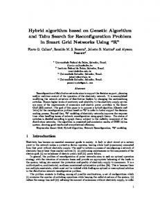
The accuracy of the model discussed in the previous section is higher compared to the n-th power model. This increase in the accuracy was achieved at the price of a bit more complex model compared to the initial model, though still much simpler compared to the BSIM3 model. Some of the parameters added to the compact model may not improve the accuracy considerably, and hence their omission leads to the simplification of the model. The flowchart of the proposed model for choosing parameters and their values is illustrated in Figure 3 which can be described briefly with the following stages ♦

GA determines which terms is used in the model,

♦

SA determines the corresponding coefficient to each term,

♦

Fitness function is calculated,

♦

If the value of Fitness function is not below a desired value, the process is repeated.

As is understood from the figure, we use the genetic algorithm to determine these less important parameters, and simulated annealing to determine the best values for the parameters. A. Genetic Algorithm The Genetic Algorithm (GA) utilizes a non-gradientbased random search and is used in the optimization of complex systems [9]. The algorithm models the process of biological evolution and optimizes the parameters of problem. In the algorithm, each unknown parameter is called gene and each vector of these parameters is called a chromosome [9]. The purpose of the genetic algorithm is to determine the elements of the unknown vector (chromosome) which maximizes or minimizes the defined fitness function. The algorithm starts with a population of chromosomes. In each generation, new population of the chromosomes is enhanced in the fitness function by means of some operators such as cross over and mutation. The initial population is chosen randomly. More details about this method can be found in [9]. In our work, this method is used to determine existing parameters.

Figure 1. The flowchart of the proposed method.

B. Simulated Annealing The Simulated Annealing (SA) is a combinational optimization technique [10]. The principle behind it is analogous to what happen when metals are cooled at a controlled rate. A typical simulated annealing process starts with a very high temperature (T), where the system state is generated at random. The cost function is analogous to the energy E(S) of a system in state S which should be minimized for the system stability. In [10], more details about this method are given. We use this method in our approach to determine the value of existing parameters.

C. Formulation of the Problem There are thirteen parameters in our proposed compact model defined in [8]. In the GA, the chromosome is defined to be a bit vector with 13 elements where each bit relates to the model parameters as follows: [K m n VT β κ λC λV σ WW WVGS p q]

(6)

If a bit becomes zero, the corresponding parameter is eliminated from the model i.e. n would be replaced by 2, p and q by 1, β, κ, λV , σ,WW, and WVGS by 0 and K , λC and VT by their physical values. Using a simple GA approach, the bit-vector chromosome can be easily determined in order to minimize the value of a goal function. In order to define the goal function, two major objectives have been considered which are the accuracy and the complexity of the model. To consider the first objective in our GA, we define the error of the model by

1 ε= NW .NVGS

∑ ∑

(7)

(8)

where δ is the number of nonzero elements in the chromosome, and η is the number of bits in each chromosome. This definition for complexity guarantees that the GA program considers minimizing the number of elements in the model to compact it. The fitness of the problem, therefore, is defined as ϕ = ε + χ .θ

T (k ) =

T0 ln k

(10)

where k is iteration number and T0 is a high starting temperature. Generating function defines as follow.

{[

(

1 λ (1 + sgn(λ − 0.5) ) X imax (k ) − X i (k ) 2 + (sgn(λ − 0.5) − 1) X i (k ) − X imin (k ) ; k = 1 : m

X i +1 (k ) = X i (k ) +

[

(

)] }

)]

(11)

where ε is the error of the model, ID,Model and ID,BSIM3 are the drain currents predicted by the compact model and the BSIM3 model (HSPICE) for the same VDS, VGS, and W, and ID,Max is the drain current at VDS = VDD, NW and NVGS are the number of sampled widths and VGS used for calculating error. For the second objective in the GA, the complexity factor is defined as δ θ= η

Annealing schemes are selected as follow:

1/ 2

 VDD   ( I D, Model − I D , BSIM 3 )2  Wmax VDD    VDS =0    I D, Max W =Wmin VGS =VT      

∑

steps. First, the objective function corresponding to the energy function must be identified. Second, one must select a proper annealing scheme consisting of decreasing temperature with increasing of iterations. Third, a method of generating a neighbor near the current search position is needed. Fourth, after a new point has been evaluated, SA decides whether to accept or reject it based on value of an acceptance function. In our optimization problem, the aforementioned functions define in (7).

(9)

where ϕ is the fitness, and χ is a weight coefficient which specifies the importance of the complexity versus the error. Having a very small χ means that the accuracy of the model is very important for the user. This leads to a model with more parameters. If χ is large enough, the model would be reduced to the α-power and n-th power models. We choose χ=1/50 to attain an average error of about 2.5%. In the SA optimization method, utilized to determine the values of the model parameters, the accepting and generating functions are the Boltzmann probability distribution and a Gaussian probability density function, respectively. The algorithm involves the following four

where sgn is the sign function, m is the number of characteristics to fit, Ximax and Ximin are the maximum and minimum of the ith dimension, and λ ∈ [0,1] . The generating function for λ has a Gaussian probability density function of

[

g (∆x, T ) = (2πT )− n 2 exp − ∆x

2

(2T )

]

(12)

The acceptance function has a Boltzmann probability distribution of h( x ) =

1 1 + exp(∆ε / cTk )

(13)

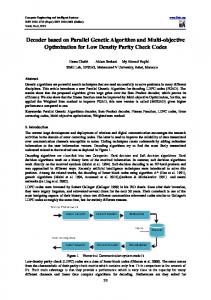
where ∆ε = ε ( X i +1 ) − ε ( X i ) and c is a system dependent constant and Tk is the temperature in kth iteration. IV. RESULTS AND DISCUSSION We have implemented the models discussed above in MATLAB. Our simulations show that for attaining 2.5% error, nine of the thirteen model parameters are required. These parameters include K, m, n, VT, β, κ, λC, WVGS, and p. The first five parameters belong to the n-th power model whereas the last four parameters have been added by the improvements that we have made to the model. The eliminated parameters were λV, σ, WW, and q. It is obvious that choosing a different value for χ could have led to another set of the model parameters. In Figures 4 and 5, the ID-VDS and ID-VGS characteristics of a NMOS transistor obtained by the proposed model and the SPICE simulations are compared which show a very good accuracy for the proposed model. The errors and the CPU time (for a 500MHz Pentium III processor) of the new and the n-th power models for NMOS and PMOS transistors (Wn = Wp = 1µm, L = 0.35µm and VDD = 3.3V) are given in Table I. As a

V. SUMMARY AND CONCLUSION We presented a compact MOSFET I-V model with the ability to modify the accuracy of the model using the genetic algorithm and simulated annealing. Using GA, one can select between the thirteen model elements based on the accuracy that needed for a specific application. For the accuracy considered in this paper, only nine elements were necessary and hence considered in the simulations. The value of each model parameter was found using simulated annealing. The results predicted by the model were compared to the results of the very accurate but complex model of BSIM3, predicting 1.3% and 3.1% of error. The very good accuracy obtained for this model suggests that for many (digital) applications, the model presented in this paper may be used in place of very complicated models like the one currently implemented in SPICE to speed up the circuit simulation.

[10] J. Roger Jang, C. Sun, and E. Mizutani, Neuro-fuzzy and soft computing, Prentice Hall, 1997. TABLE I. COMPARISON OF BSIM3, N-TH POWER AND PROPOSED MODEL

Model Error (PMOS) Error (NMOS) CPU time (ms) This Model 3.1% 1.3% 0.3 n-th power 7.5% 3.7% 0.2 BSIM3 10 -4

x 10 6

Vgs=3 V

4

ID (A)

reference, the required time of BSIM3 is also given in this table. The times required for the compact models are much smaller compared to the BSIM3 model while having few percents of error.

2

Vgs=2 V

0

Vgs=1 V 0

REFERENCES

0.5

1

Vds (V)

1.5

2

Figure 2. The ID-VDS characteristic of a NMOS transistor [1] [2] [3]

[4] [5] [6]

[7] [8]

[9]

A.P. Chandrakasan, W.J. Bowhill and F. Fox, Design of Highperformance Microprocessor Circuits, IEEE Press. 2001. D.P. Foty, MOSFET modeling with SPICE, principles and practice, Prentice Hall, 1997. T. Sakurai and R. Newton, “Alpha-power low MOSFET model and its application to CMOS inverter delay and other formulas,” IEEE J.l of Solid-State Circuits, vol. 25, pp. 584-594, Apr. 1990. T. Sakurai and A.R. Newton, “A simple MOSFET model for circuit analysis,” IEEE Trans. Electron Device, vol. 38, pp. 887-894, 1991. W. Shockley, “A unipolar filed effect transistor,” Proc. IRE, vol 40, pp. 1365-1376, Nov. 1952. R. Van Langevelde and F.M. Klaassen, “Accurate drain conductance modeling for distortion analysis in MOSFETs,” IEDM 1997 Tech. Digest, pp. 313-316, 1997. Y. Tsividis, Operation and modeling of the MOS transistor, McGrawHill, 1999. M. Taherzadeh-Sani, A. Abbasian, B. Amelifard, and A. AfzaliKusha, “MOS Compact I-V Modeling with Variable Accuracy Based on Genetic Algorithm and Simulated Annealing,” in Proceedings of the 16th International Conference on Microelectronics, Tunis, Tunisia, December 6-8, pp. 364-367, 2004. D. E. Goldenberg, Genetic algorithm in search, optimization and machine learning, Addison Wesley, Reading MA, 1989.

(W=1µm, L=0.35 µ and VDD=3.3V).

Figure 3. The ID-VGS characteristic of a NMOS transistor (W=1µm, L=0.35 µm and VDD=3.3V).