Mar 6, 2008 - equispaced points to generate a look-up table for psd as a function of t. (iii) Create a histogram of t and smooth it with a low- ..... pub-9165.html.
PHYSICAL REVIEW SPECIAL TOPICS - ACCELERATORS AND BEAMS 11, 030701 (2008)
Modeling of the microbunching instability M. Borland ANL, Argonne, Illinois 60439, USA (Received 4 December 2007; published 6 March 2008) We show that, through careful control of noise sources, it is possible to determine the microbunching gain curve for the FERMI@ELETTRA linac using the particle tracking code ELEGANT. In addition to using a sufficiently large number of particles (60 � 106 ), use of a low-pass filter is very helpful in controlling noise and providing convenient intrabin interpolation. Gains of up to 1500 are seen for modulation wavelengths down to 25 �m. Because of the high gain, very small initial modulations are needed to avoid saturation, which further motivates the use of a large number of particles. We also show, for the first time, how the density modulation evolves in detail inside the dipoles of a multichicane system. DOI: 10.1103/PhysRevSTAB.11.030701
PACS numbers: 29.20.�c, 29.27.�a, 41.60.Ap
I. INTRODUCTION That coherent synchrotron radiation (CSR) generated by short bunches in magnetic bunch compressors and other bending systems may degrade beam quality has been known for more than a decade [1]. Magnetic bunch compression is a common feature of linacs designed as drivers for free-electron lasers (FELs), for example, the Linac Coherent Light Source (LCLS) [2] and FERMI [3] projects. At one time, it was thought that the most important effect of CSR was to increase the projected beam emittance and energy spread. However, simulations [4,5] with the code ELEGANT [6] predicted in addition a CSRdriven microbunching instability that may have a dramatic impact on FEL performance. In addition to CSR, it was discovered [7] that longitudinal space charge (LSC) can lead to a potentially more serious microbunching instability when combined with bunch compression and CSR. Various suppression mechanisms were identified, such as use of a superconducting wiggler [2] or ‘‘laser-undulator beam heater’’ [8] to increase the slice energy spread of the beam. In this paper, we simulate CSR- and LSC-driven microbunching instabilities in the FERMI linac, using the lattice from April 2007 [9] and the parallel version of ELEGANT [10]. (Note that the lattice ends with the final bunch compressor, i.e., it does not include the vertical ‘‘dog-leg’’ at the end of the linac.) We discuss the simulation methods, in particular, issues of noise control. We exhibit gain curves for the instability over a range of initial modulation wavelengths.
II. PREPARING THE INITIAL PARTICLE DISTRIBUTION Typically modeling with ELEGANT begins at about 100 to 150 MeV. Below that energy, a code such as PARMELA [11], ASTRA [12], or GPT [13] is used, since these codes have detailed models of space-charge effects and can per1098-4402=08=11(3)=030701(8)
form accurate injector modeling. Often these codes are run with 200 to 500 thousand particles, due to code limitations or in order to limit running times. It was determined [14] that the appearance of the instability in ELEGANT simulations of LCLS resulted from noise in the input particle distribution generated with the code PARMELA. In other words, for a sufficiently quiet input beam, the instability did not appear. Given this, one might reasonably question whether the instability is a valid prediction. To answer this in detail, one needs to systematically inject density modulations into the beam and determine the gain curve of the instability [14]. One may also draw on common experience in the accelerator control room, where one frequently observes electron and drive laser beams that exhibit much more structure than the typical perfectly smooth Gaussians and beer cans used in simulations. Analysis of the instability gain requires that we start with a much quieter distribution than available from typical photoinjector simulations. To accomplish this, we wrote a self-describing data sets (SDDS)-based script SMOOTHDIST6 that smooths particle distributions in 6dimensional phase space �x; x0 ; y; y0 ; t; p�. The sequence of operations performed by the script is listed below. Many of the numerical parameters used in the script are obtained by trial and error, based on examination of the noise levels in the resulting distribution and the degree to which it reproduces features in the original distribution. (i) Fit a 12th-order polynomial to p as a function of t. Evaluate the polynomial at 10 000 equispaced points to generate a look-up table for the momentum variation with time. (ii) Compute the standard deviation of the momentum psd for blocks of 2000 successive particles. Fit this data with a 12th-order polynomial and evaluate it at 10 000 equispaced points to generate a look-up table for psd as a function of t. (iii) Create a histogram of t and smooth it with a lowpass filter having a cutoff at 0.1 THz. This may result in
030701-1
© 2008 The American Physical Society
M. BORLAND
Phys. Rev. ST Accel. Beams 11, 030701 (2008)
ringing at the ends of the histogram, which is clipped off by masking with the original histogram. (iv) Optionally modulate the histogram H�t� with a sinusoid, by multiplying the histogram by 1 � dm cos�2�ct=�m �, where dm is the modulation depth and �m is the modulation wavelength. For nonzero dm , this will result in a longitudinal-density-modulated distribution when the histogram is used as a probability distribution and sampled to create time coordinates. (v) Sample the time histogram N times using a ‘‘quiet start’’ Halton sequence [15] with radix 2, where N is the number of desired particles. The sampling operation is performed by first numericallyR computing the R cumulative 0 0 distribution function C�t� � t�1 H�t0 �dt0 = 1 �1 H�t �dt . Inverting this to obtain t�C�, we generate each sample from H�t� by evaluating t�U�, where U is a quantity on the interval [0, 1] generated from the Halton sequence (vi) Create samples for other coordinates by quiet sampling of Gaussian distributions: (a) Scaled transverse co^ x^ 0 , y, ^ and y^ 0 using Halton radices 3, 5, 7, and ordinates x, 11, respectively. For convenience in scaling [step (ix)], these are defined such that the standard deviation of each coordinate is 10�4 and all coordinates are uncorrelated. (b) Scaled fractional momentum deviation �1 using Halton radix 13, with unit standard deviation. (vii) Interpolate the look-up tables to determine the mean pmean and standard deviation psd of the momentum at each particle’s time coordinate. Use these to compute the individual particle momenta using p � pmean � �1 psd . (viii) Compute the projected transverse rms emittances and Twiss parameters for the original beam. (ix) Transform the scaled transverse phase-space coordinates to give the desired projected Twiss parameters in the x and y planes. The x and y planes are assumed to be uncorrelated. As mentioned, the numerical parameters of this procedure are determined by trial and error. A particular difficulty is to smooth the longitudinal density sufficiently to control noise and residual density ripples while not removing important features. Figure 1 shows that using the parameters above we successfully reduced noise, resulting in a very smooth distribution. However, we also removed some apparently real features at the ends of the distribution. Fortunately, these features are unimportant as they get folded into the current spikes and the ends of the pulse. We are not much interested in this region as the beam there is not useful. One alternative to six-dimensional smoothing would be to perform a purely two-dimensional simulation, i.e., using only the longitudinal phase-space coordinates. This might seem reasonable given that the CSR and LSC models act directly only in the longitudinal plane. However, this is not advisable for several reasons. First, the longitudinal space charge depends on the beam size, so this would have to be artificially included if we track in the longitudinal plane only. Second, by performing six-dimensional tracking, we
FIG. 1. (Color) Longitudinal density before (black) and after (red) smoothing and resampling.
automatically include important gain-reducing effects from the emittance and energy spread of the beam [8,16]. III. MODELING METHODS The models used for CSR [17–19] and LSC [8] have been presented previously. In brief, in both cases we make use of a line-charge model to compute the longitudinal forces on the beam from the current density ��t�. These models involve, either explicitly or implicitly, derivatives of ��t�, which give rise to energy modulation when there are local current density fluctuations, particularly at short wavelengths. This effect, combined with path-length dispersion in bending systems, is the fundamental source of the instabilities. In the context of simulation with ELEGANT, the current density is computed by binning simulation particles. With a finite number of particles, it is not possible to entirely avoid binning noise. This is true even though the smoothed distribution is sampled using a Halton sequence. There are three reasons for this. One is that, with a finite number of particles, one cannot avoid statistical fluctuations in the number of particles in adjacent bins when a large enough number of bins is used. This is particularly the case when the longitudinal distribution is evolving, since that means particles are moving between bins. A second reason is that the beam transport exhibits coupling between the various phase-space coordinates. In particular, there is coupling among the momentum, time, and horizontal coordinates inside the chicane. This can result in modulations developing in the current histogram due to banding in the Halton sequences for different radices, for example. Figure 2 illustrates the banding issue. Banding is worst when the ratio of the radices is close to unity. For this reason and in light of the strong coupling between the time and momentum coordinates in the system under study, we used radix 2 for time and radix 13 for
030701-2
MODELING OF THE MICROBUNCHING INSTABILITY
Phys. Rev. ST Accel. Beams 11, 030701 (2008)
FIG. 3. (Color) Illustration of the effect of nearest-neighbor smoothing in the frequency domain. FIG. 2. Illustration of banding in longitudinal phase space when Halton radices of 11 and 13 are used for time and momentum coordinates, respectively. Banding becomes less evident as the number of particles is increased and when the ratio of the radices is far from unity.
momentum, respectively, which reduces the banding significantly. In passing, we note that if, say, a Halton sequence was used for the time coordinate and a pseudorandom-number sequence was used for x, the random noise from the x coordinate would get coupled into the longitudinal plane. It is essential to use quiet start sequences for all coordinates. A third source of noise is that the beam emits ordinary synchrotron radiation in the dipole magnets, which entails noise due to quantum excitation. With a relatively small number of particles, this noise is exaggerated relative to the real case, something which becomes apparent when we compute histograms or statistics. (This is because the simulation particles in a code like ELEGANT are not ‘‘macroparticles.’’ Rather, they are representative electrons. The Appendix comments further on this point.) If uncontrolled, noise from these sources can be amplified by CSR and LSC, resulting in a false indication of an unstable situation. There are several steps that may be taken to reduce these effects, for example, using more particles, using fewer bins, and applying smoothing to the histogram. We begin with a discussion of smoothing, which is a very common approach. Often this is done in a fairly simple way, for example, replacing each bin with the average of itself and its nearest neighbors. To illustrate the pitfalls in this, we generated 2048 uniformly distributed random numbers on ��1; 1�. Taking the fast-Fouriertransform of this sequence, we get a nominally uniform noise level as a function of frequency. Figure 3 shows how ineffective nearest-neighbor smoothing is at reducing noise at high frequencies. Clearly, any effect in the simulation that preferentially amplifies high-frequency noise will not be effectively suppressed by simple nearest-neighbor smoothing. Using higher-order smoothing filters, e.g., a
second-order Savitzky-Golay [20,21] filter, is better but still inadequate. For example, we have observed that higher-order Savitzky-Golay filters merely introduce additional notches in the frequency spectrum, without fully suppressing the high frequencies. To deal with these issues in ELEGANT, we have taken a more direct approach to noise control for CSR and LSC. In particular, the user simply specifies an idealized low-pass filter, described as 8 f < c1 fN < 1; f�c2 fN F�f� � �c1 �c2 �fN ; c2 fN f c1 fN (1) : 0; f > c2 fN ; where 0 < c1 < c2 < 1 and fN is the Nyquist frequency. Typically, we would choose c1 � 1=5 and c2 � 1=4, meaning that the filter would start to fall linearly from 1 at f � 0:2fN and be 0 at f � 0:25fN . One might question whether this procedure is any better than simply using four or five times fewer bins. The reason it is superior is that the filtering process provides interpolation as well as noise control. If fewer bins are used, we must devise a method for interpolating within bins in order to avoid stair-step effects. This can be quite difficult if the signal is not sampled sufficiently often, since one may be forced to use higher-order interpolation to get smooth variation. On the other hand, if we bin more finely and use a low-pass filter, we automatically get smooth variation of the signal and can confidently apply a simple linear interpolation within bins. Figure 4 illustrates these points. Having understood how to set the filter, we must still set the number of bins in the histograms used for computing CSR and LSC effects. The beam from the FERMI photoinjector spans 15 ps. Based on experience with LCLS, we are interested in wavelengths well under 100 �m. Choosing 2000 bins puts the Nyquist frequency at 67 THz or 4:5 �m. Our noise filter with c1 � 1=5 and c2 � 1=4 would thus remove noise at and below 22 �m. Thus, we might reasonably expect to perform simulations with density modulations as short as 25 �m.
030701-3
M. BORLAND
Phys. Rev. ST Accel. Beams 11, 030701 (2008)
FIG. 4. (Color) Illustration of why finer sampling combined with filtering is superior to coarse sampling. The original signal is a sinusoid to which 10% random noise is added. A filter is applied with c1 � 1=5 and c2 � 1=4, giving the ‘‘Filtered’’ signal. This is compared to a pure sinusoid that is simply sampled 1=5 as often.
With this large number of bins, use of a low-pass filter alone is not sufficient to control noise in the simulations. Figure 5 shows final longitudinal density for various numbers of macroparticles with the noise filter turned on. We see that, even with 1 � 106 particles, there is still a severe instability. Increasing this by an order of magnitude to 10 � 106 particles dramatically reduces the problem. To illustrate the role of the noise filter even when the number of particles is at this level, Fig. 6 compares the results with and without the noise filter for 20 � 106 particles. Even with the filter turned on, there is still evidence of instability. In view of this, we elected to use 60 � 106 particles in our
FIG. 6. (Color) Final longitudinal density for FERMI, showing the effect of the low-pass filter when 20 � 106 particles are used.
production simulations, which is the maximum that can be run given the memory (16 GB) on our cluster’s head node. To ensure reliable results, we must ensure that the final modulation in our simulations is well above this residual noise level and also show that results are reasonably stable as the number of particles is varied. This will indicate that a sufficient number of particles has been used. Evidence of this is shown below. Another reason to use a large number of particles is the desire to simulate very small initial modulations. As we will see, the gain for 25 �m is about 1500. To stay within the quasilinear regime we would like to have a final modulation of about 20% or less. This requires having an initial modulation of about 0:013%. With 2000 bins, the number of particles per bin on average is about 3 � 104 . A 0:013% modulation thus corresponds to having only 8 more particles in the most populated bin compared to the least populated nearby bin. Although this seems marginal, results show that it is in fact quite acceptable. This can be understood by realizing that we are really looking at a modulation that includes many periods, so the signal is in this sense larger than the number of particles might make it seem. IV. SIMULATION RESULTS AND DISCUSSION
FIG. 5. Final longitudinal density for FERMI, showing the result of increasing the number of particles from 200 000 to 10 � 106 .
Having understood how to control noise in the input distribution and simulation, we are in a position to determine a gain curve for the system. To do this, we create a series of beam files using SMOOTHDIST6, with modulation wavelengths �m beginning at 25 �m and ending at 100 �m. Because we do not know the gain ahead of time, we must vary the initial modulation depth dm . Although this significantly increases the total computational effort, it provides additional information that validates the simulations, as we will see. Figure 7 shows final longitudinal densities for initial 30-�m modulations of various amplitudes. For an initial
030701-4
MODELING OF THE MICROBUNCHING INSTABILITY
FIG. 7.
Phys. Rev. ST Accel. Beams 11, 030701 (2008)
Final longitudinal density for FERMI for 30 �m initial modulations of various amplitudes.
density modulation of less than 0.025%, the final density modulation is under 20%. At an initial density modulation of 0.05%, the final density modulation is essentially 100%. It appears to decrease after this, but this is misleading. In fact the effect has saturated and is producing harmonics. This can be seen in Fig. 8, where we show only the central 100 bins of the histograms. Only for the smallest initial modulation is the final modulation reasonably sinusoidal. In all other cases, considerable distortion is seen, with obvious harmonics appearing for 0.2% or higher. The fact that the final modulation is reasonably sinusoidal and regular indicates that we can reliably compute the gain. To obtain the gain curve from such data, we must determine the modulation amplitude at the end of the
system from each run. The ratio of this amplitude to the initial amplitude is the apparent gain (ignoring saturation). We started by making 2000-bin histograms of the final time coordinate, then removed the leading and trailing 500 bins to eliminate end effects. We fit a 7-term polynomial to the remaining data to obtain the average value from the constant term of the fit. Finding the residuals of the fit gives us data that contains only the fast variations related to the initial modulation and, perhaps, noise. Subjecting this data to numerical analysis of fundamental frequencies (NAFF) gives the frequency of the modulation and its amplitude. Dividing the latter by the average value of the density gives the fractional modulation depth. The ratio of the initial
FIG. 8. (Color) Final longitudinal density for FERMI for 30 �m initial modulations of various amplitudes, showing only the central 100 bins.
FIG. 9. (Color) Wavelength compression factor of FERMI as a function of the initial wavelength of the density modulation and its depth. Values in excess of 10 are not shown.
030701-5
M. BORLAND
Phys. Rev. ST Accel. Beams 11, 030701 (2008)
FIG. 10. (Color) Modulation gain factor of FERMI as a function of the initial wavelength of the density modulation and its depth. FIG. 11. Dependence of the computed gain on the number of particles for an initial modulation of 0.05% at 30 �m.
frequency of the modulation to the final frequency gives the compression factor of the system, providing a valuable check that the analysis has been performed correctly. Figure 9 shows the compression factor as a function of initial wavelength for various modulation depths up to 2%. We see a fairly consistent result of between 9.0 and 9.4, with some aberrant values for high initial amplitudes, particularly at short wavelengths. Figure 10 shows the gain values, which have a much more interesting pattern. For large initial amplitude, as we go from long to short wavelengths, the apparent gain rolls off at relatively long wavelengths. This effect diminishes as the initial amplitude is decreased, until for amplitudes under 0.03% the results converge even for the shortest initial wavelength. This convergence represents not only a convergence of the simulation, but also reflects the elimination of saturation effects. To further demonstrate convergence of the simulations, we need to vary the number of particles. This is a challenge because we must choose a sufficiently small initial density modulation to prevent saturation without making the modulation so small that it is ineffective in the cases with fewer particles. A good choice for this is a modulation wavelength of 30 �m with a modulation depth of 0.05%, since this is a relatively short wavelength and 0.05% is the largest modulation depth (for this wavelength) for which the gain result has approximately converged as a function of modulation depth. Figure 11 shows the results of varying the number of particles from 2 � 106 to 60 � 106 , which demonstrates convergence of the simulation with a fairly small number of particles. For 10 � 106 particles or more, the variation in the gain is less than 3%. The use of 60 � 106 particles was based on the desire to suppress obvious noise in the final distributions, which is unnecessarily stringent for gain curve determination. The reason is that the NAFF analysis used on the final distribution provides additional protection against noise for gain curve studies, since it selects out the dominant frequency and thus to a
significant extent ignores noise. This is discussed further below. It is interesting to look at the evolution in the modulation depth as a function of location in the accelerator. ELEGANT allows us to do this conveniently because it provides optional SDDS output of longitudinal density histograms at each slice in the dipole. (These histograms are computed as part of the CSR simulation.) These are readily analyzed to obtain the density modulation at the end of each slice, just as was done for the final density modulation to produce the results shown above. Figure 12 shows the evolution for three cases: no initial modulation, an initial modulation of 0.0125% at 25 �m, and an initial modulation of 0.025% at 25 �m. When the three curves coincide, we know that the density modulation is below the noise level of the simulations.
FIG. 12. (Color) Evolution of the modulation amplitude in FERMI as a function of location in the dipoles of the chicanes, for three cases: no initial modulation, 0.0125% initial modulation at 25 �m, and 0.025% initial modulation at 25 �m. Dipole 1 is the first dipole in the first chicane, dipole 4 is the first dipole in the second chicane, and so on. Linac structures exist between dipoles 4 and 5, and between dipoles 8 and 9.
030701-6
MODELING OF THE MICROBUNCHING INSTABILITY We see that the density modulation is quickly ‘‘washed out’’ in dipole 1, only to rise above the noise level at the end of dipole 2 and dipole 4. The washed-out modulation reappears because, before washing out, it imposes an energy modulation on the beam. In the second chicane (dipoles 5 through 8), a density modulation makes a brief, stronger appearance in dipole 7, but quickly washes out. In this case, the density modulation grows quickly from incoming energy modulation combined with path-length dispersion in the dipole, but washes out because of the size of the energy modulation and accumulation of pathlength dispersion. However, this does not happen before CSR imposes a new energy modulation that grows again into density modulation within dipole 8, resulting in a very large density modulation entering the linac (between dipoles 8 and 9). These patterns demonstrate that the energy modulation produced in the linac, while important, is not directly responsible for the larger density modulation at the exit of the chicane. Instead, there is a complex exchange of energy and density modulation inside the chicane, seeded by the energy and density modulation at the entrance, and mediated by path-length dispersion and CSR. This figure also serves to illustrate the degree to which the signal from the initial modulation rises above the noise at the end of the system, which is relevant to determining the overall gain. Since the noise is a factor of 5 to 10 below the signal level, the detection of the signal is extremely reliable. The NAFF algorithm picks out only the strongest, most persistent signal in the data, and can reliably detect signals that are buried in noise. Tests showed that for 1000point sequences like those used in our analysis, the amplitude and frequency of a sinusoidal modulation was reliably detected even when uniformly distributed random noise was added with 5 times higher peak-to-peak amplitude. Only when the signal is smaller than this did detection begin to fail. Hence, detection of signals with amplitudes seen in these simulations is very reliable. Although not evident from Fig. 12, the detected wavelength is essentially random for the data with no initial modulation. This is also true for those points where the amplitude from the modulated cases overlays the data from the unmodulated case, but not in those cases where the former strongly departs from the latter. Hence, checking for a reasonable detected frequency is an excellent quality control measure and is part of the algorithm for determining the gain in Fig. 10. V. CONCLUSION We have shown how, through careful control of noise sources and judicious data analysis, it is possible to determine the microbunching gain curve for the FERMI@ELETTRA linac using the particle tracking code ELEGANT. In addition to using a sufficiently large number of particles (up to 60 � 106 ), use of a judicious low-pass filter is very helpful in controlling noise and
Phys. Rev. ST Accel. Beams 11, 030701 (2008) providing convenient intrabin interpolation. Using NAFF to detect the signal resulting from the initial modulation provides additional noise immunity and quality control. Gains of up to 1500 are seen for modulation wavelengths down to 25 �m. Because of the high gain, very small initial modulations are needed to avoid saturation, which further motivates the use of a large number of particles. We have also shown, for the first time, how the density modulation evolves in detail inside the dipoles of a multichicane system. ACKNOWLEDGMENTS The author acknowledges Yusong Wang, the developer of parallel ELEGANT, for code developments that permitted large-particle runs. The author also acknowledges Robert Soliday for implementing changes to the Linux cluster that made it possible to run large numbers of particles efficiently. The submitted manuscript has been created by UChicago Argonne, LLC, Operator of Argonne National Laboratory (Argonne). Argonne, a U.S. Department of Energy Office of Science laboratory, is operated under Contract No. DE-AC02-06CH11357. APPENDIX: COMMENT ON THE MACROPARTICLE CONCEPT It is common to refer to the simulated particles in a tracking code as ‘‘macroparticles.’’ The implication is that each macroparticle represents some large number of actual electrons. However, when including effects such as quantum excitation, the statistics we use are those for a single electron, which is inconsistent. The macroparticle concept is, in fact, erroneous in this case. We do not simulate ‘‘super electrons’’ with N � 1 times the charge and mass of real electrons. Instead, we simulate actual electrons, but only a small sample of the electrons that are present in a real beam. If a sufficient number of simulation electrons are used, their statistics will accurately reflect the statistics of the real beam. To the extent that we use fewer simulation particles than are present in the real beam, we exaggerate noise effects and must employ various strategies, such as quiet start sequences and low-pass filtering, to reduce the noise. This way of thinking appears to contradict the common method for simulation of collective effects, which involves attributing N times the normal electron charge to each simulated electron. However, this is not the case. When we compute collective effects, we begin by preparing a histogram of the particle distribution, for example, the line number density N�s�. We implicitly assume that the distribution of the simulation particles is, for a sufficiently large number of simulation particles, close to the actual distribution. We can then multiply the simulated N�s� by the ratio of actual particles to simulation particles, to get an approximation to the real beam distribution. Having done
030701-7
M. BORLAND
Phys. Rev. ST Accel. Beams 11, 030701 (2008)
so, we then compute the effect on each simulation particle of the approximate wakefield, CSR field, or space charge (for example) of the real beam.
[1] B. E. Carlsten and T. O. Raubenheimer, Phys. Rev. E 51, 1453 (1995). [2] Linac Coherent Light Source (LCLS) Conceptual Design Report, SLAC Report No. SLAC-R-593, 2002. [3] G. D’Auria et al., Proceedings of LINAC2002, 641–643; http://www.elettra.trieste.it/FERMI/. [4] M. Borland et al., Proceedings of the 2001 Particle Accelerator Conference, pp. 2707–2709 (2001). [5] M. Borland et al., Nucl. Instrum. Methods Phys. Res., Sect. A 483, 268 (2002). [6] M. Borland, Advanced Photon Source LS-287 (2000). [7] E. L. Saldin et al., DESY Report No. TESLA-FEL-200302, 2003. [8] Z. Huang et al., Phys. Rev. ST Accel. Beams 7, 074401 (2004). [9] S. Di Mitri (private communication). [10] Y. Wang et al., Proceedings of the 2007 Particles Accelerator Conference, pp. 3444 –3446 (2007).
[11] L. Young and J. Billen, PARMELA code (http://laacg.lanl. gov/laacg/services/parmela.html). [12] K. Floettmann, https://www.desy.de/ mpyflo. [13] S. B. van der Geer and M. J. de Loos, http://www.pulsar.nl/ gpt. [14] M. Borland et al., Proceedings of the 2002 Linac Conference, pp. 11–15 (2002). [15] J. Halton, Numer. Math. 2, 84 (1960). [16] S. Heifets et al., Report No. SLAC-PUB-9165, 2002, http://www.slac.stanford.edu/pubs/slacpubs/9000/slacpub-9165.html. [17] E. L. Saldin et al., Nucl. Instrum. Methods Phys. Res., Sect. A 398, 373 (1997). [18] M. Borland, Phys. Rev. ST Accel. Beams 4, 070701 (2001). [19] G. Stupakov and P. Emma, Report No. SLAC-PUB-9242, 2002. [20] W. H. Press, S. A. Teukolsky, W. T. Vetterling, and B. P. Flannery, Numerical Recipes in C (Cambridge University Press, Cambridge, England, 1992), 2nd ed. [21] A. Savitzky and M. J. E. Golay, Anal. Chem. 36, 1627 (1964).
030701-8