Modeling spatial distribution of Tehran air pollutants using ... - Pollution

Pollution, 2(4): 375-386, Autumn 2016 DOI: 10.7508/pj.2016.04.001 Print ISSN 2383-451X Online ISSN: 2383-4501 Web Page: https://jpoll.ut.ac.ir, Email: [email protected]

Modeling spatial distribution of Tehran air pollutants using geostatistical methods incorporate uncertainty maps Halimi, M.1*, Farajzadeh, M.1 and Zarei, Z.2 1. Department of Climatology, TarbiatModares University, Tehran, Iran 2. Department of Climatology, Lorestan University, Iran Received: 9 Nov. 2015

Accepted: 23 Jul. 2016

ABSTRACT: The estimation of pollution fields, especially in densely populated areas, is an important application in the field of environmental science due to the significant effects of air pollution on public health. In this paper, we investigate the spatial distribution of three air pollutants in Tehran’s atmosphere: carbon monoxide (CO), nitrogen dioxide (NO2), and atmospheric particulate matters less than 10 μm in diameter (PM10μm). To do this, we use four geostatistical interpolation methods: Ordinary Kriging, Universal Kriging, Simple Kriging, and Ordinary Cokriging with Gaussian semivariogram, to estimate the spatial distribution surface for three mentioned air pollutants in Tehran’s atmosphere. The data were collected from 21 air quality monitoring stations located in different districts of Tehran during 2012 and 2013 for 00UTC. Finally, we evaluate the Kriging estimated surfaces using three statistical validation indexes: mean absolute error (MAE), root mean square error (RMSE) that can be divided into systematic and unsystematic errors (RMSES, RMSEU), and D-Willmot. Estimated standard errors surface or uncertainty band of each estimated pollutant surface was also developed. The results indicated that using two auxiliary variables that have significant correlation with CO, the ordinary Cokriginga scheme for CO consistently outperforms all interpolation methods for estimating this pollutant and simple Kriging is the best model for estimation of NO2 and PM10. According to optimal model, the highest concentrations of PM10 are observed in the marginal areas of Tehran while the highest concentrations of NO2 and CO are observed in the central and northern district of Tehran. Keywords: air pollution, geostatistical schema, Kriging, uncertainty map, Tehran.

INTRODUCTION* Air pollution in urban areas has serious health and quality of life implications. A wide variety of anthropogenic air pollution sources increase the levels of background air pollutant concentrations. Among the world’s top 10 most polluted cities, four are in Iran. Tehran, capital of Iran, suffers from severe air pollution and the city is often covered by *

smog making breathing difficult and causing widespread pulmonary illnesses. It is estimated that about 27 people die each day from pollution-related diseases in Tehran. In 2013, the Health Ministry of Iran announced that up to 4,460 Tehran residents died due to air pollution, equivalent to roughly 25% of the total number of deaths in the city each year. Dust is a primary cause of air pollution. Air pollution is usually caused by natural

Corresponding author E-mail: [email protected]

375

Halimi, M. et al.

events and/or anthropogenic activities. Major man-made activities include automobiles, power generation, and industrial activities, in particular, oil refineries, which represent the main source of air pollution (Salwan et al., 2016). Main sources of Tehran air pollution are vehicular that produce nearly 0.75 of Tehran's air pollution (Brajer et al., 2012). Most of the approximately 2 million motor vehicles in Tehran are more than 20 years old and many lack catalytic converters (Halek et al., 2004; Halek et al., 2010). Others include industrial activity and, in general, fossil fuel combustion. The deterioration of urban air quality is considered as one of the primary environmental issues and current scientific evidence associates the exposure to ambient air pollution with a wide spectrum of health effects such as cardiopulmonary diseases, respiratory-related hospital admissions, and premature mortality (Liang et al., 2009; Rajarathnam et al., 2011; Ito et al., 2005). Atmospheric pollution in urban centers has been one of the main causes of human illness related to the respiratory and circulatory system (Weeberb et al., 2015). Pollutants like carbon monoxide, sulfur dioxide, and the aerosols that are known to be among the most important factors related to heart, vascular, and lung disease, have underlined public welfare and health, and the organizations concerned with community health undertake remarkable expenses for disease coming out of these pollutants per year. Awareness of the air situation and its quality over periods and the process of air pollutants’ changes in locations, and especially detection of high risk places can play an important and efficient role in urban health management and land use policymaking (Kavousi et al., 2013). Real-time assessment of the ambient air quality has gained increased interest in recent years (Gerbole et al., 2011). Giving support to this evolution, the Geostatistical air

pollution interpolation model (GAPIM) was developed (Samet et al., 2000). GAPIM was applied in air pollution modeling for estimating the spatial distribution of pollutants, based on data provided from an existing air quality monitoring network or stations. MATERIALS AND METHODS The study area, city of Tehran, which is located in northern part of Iran (between 35.56–35.83N and 51.20–51.61E; Fig. 1), is a polluted Middle East city. The city is divided into 22 districts. The total area of Tehran is about 700 Km2. Tehran is bordered by the Alborz mountains to the north. Approximately 10 million people live in Tehran area. Rapid urbanization over the past several decades has contributed to a significant increase in population (Rashid, 2011; Kakooei and Kakooei, 2007). In this study, we use two years average (2012 and 2013) data of 3 air pollutants in Tehran’s atmosphere, namely carbon monoxide (CO in ppm), nitrogen dioxide (NO2 in ppb), and atmospheric particulate matters less than 10 μm in diameter (PM10 μm in M-3). The data are collected from 22 air quality monitoring stations which are located in different district of Tehran. The Kriging interpolation schemes are stochastic, local, gradual, and exact interpolators (Janssen et al., 2008). The Kriging methodology includes two stages: the analysis of the spatial variation and the estimation of the target variable, which is also based on the weighted average approach (Avellaneda, 2007). The analysis of the spatial variation is performed through the variogram assessment. The Kriging scheme is also known as the best linear unbiased estimator, and its estimates are based on the variogram model and the values and location of the measured points (Moscato et al., 2011).

376

Pollution, 2(4): 375-386, Autumn 2016

N

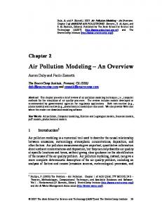
Fig. 1. Satellite Image of Tehran (capital of Iran) which surrounded in north by Alborz mountain range. The 22 districts of Tehran city and location of monitoring air quality stations are shown in this image (green circle).

The Kriging interpolation weights are chosen using the modeled semivariogram so that the estimate is unbiased and the estimation variance is less than any other linear combination of the observed values (Gretchen et al., 2012). In this paper, we use 4 most common Kriging methods, namely simple Kriging (SK), which assumes a known constant mean, ordinary Kriging (OK), which assumes that there is an unknown constant mean estimated from the data, universal Kriging (UK), which assumes that there is a trend in the surface that partly explains the data’s variations, and Ordinary Cokriging (OCK), in which the auxiliary variables can be used for estimation. In this paper, we use statistical approach (versus deterministic approach) which enables the prediction of uncertainty bands associated with the predicted surfaces as:

KSE  Z  x   1.96  σ

(1)

where KSE is Kriging standard errors, (x) is Kriging Predictor, σ is the Kriging variance, and the value 1.96 comes from the standard normal distribution where 0.95 of probability is contained from ±1.96. A rule of thumb is that 0.95 of the time the observed value of pollutant concentration will be within the interval formed by taking the estimated value is ±1.96 times the prediction standard error if data are normally distributed. Interpolation methods performance testing was done by cross validation algorithm (Wong et al., 2004). Willmott (1984) used five difference measures that are useful in evaluating the performance of the interpolation methods. These measures are: 377

Halimi, M. et al.

1. mean absolute error (MAE),

estimated value of pollutant concentration for 22 air pollution monitoring stations (N), respectively, and xo is the average of observed data. MAE is sometimes preferred over the RMSE as an evaluator because it is less sensitive to extreme values (18); however, RMSE is the error measure commonly computed in geographic applications. RMSEs assesses whether the model errors are predictable, whereas the RMSEu identifies those errors that are not predictable mathematically. Where Pˆi  a  b  Xoi  and a and b are coefficient of an ordinary leastsquare (OLS) simple linear regression between Xo (observed data as dependent variable) and Xp (estimated data by fitted GAPIM as independent variable). The final error measure, d, varies between 0.0 and 1.0. Therefore, the closer d is to 1.0, the better the agreement between Xo and Xp with 1.0 conveying perfect agreement and 0.0 complete disagreements (Wong et al., 2004). The methodological processes are shown in Figure 2.

MAE  N 1   x o  x p  n

i 1

2. root mean square errors (RMSE), n

RMSE  N 1 {(x o  x p )2 }1/2 i 1

3. systematic root mean square errors (RMSEs), N



RMSEs  N 1   Pˆi  x o  i 1 

 

2 1/2

4. unsystematic root mean square errors (RMSEu), N





1/2

2 RMSEu  N 1   x p  Pˆi    i 1 

5. The index of agreement (d-Willmote). d  1  N * RMSE 2 / PE n

PE  ( x p  xo  x o  xo ) 2 i 1

where Xo and Xp are observed and

Fig. 2. The methodological processes of modeling spatial distribution of air pollutant concentration in Tehran

378

Pollution, 2(4): 375-386, Autumn 2016

RESULTS The spatial trend of three air pollutants in Tehran’s atmosphere have been shown in the trend analysis diagram in Figure 3. According to this diagram, which its X-axis is East-West direction and Y-axis is SouthNorth direction, the concentration of CO in Tehran’s atmosphere along X-axis has an increasing trend toward central district of Tehran and decreasing trend to eastern and western district (parabolic trend) and along Y-axis has constant increasing trend toward northern part of Tehran (logarithmic trend). PM10 concentration also has logarithmic decreasing trend toward west of Tehran and

also decreasing parabolic trend toward southern part of Tehran. The NO pollutant, as can be seen in the Figure 4, follows a spatial trend just like CO. After detecting spatial trends of mentioned air pollutants in Tehran’s atmosphere, we use second order de-trending model removing these spatial trends. The correlation matrix of 7 measured air pollutants in 21 air quality monitoring stations has been shown in Table 1. We use this correlation matrix determining auxiliary variable in ordinary Cokriging interpolation method.

Fig. 3. Spatial Trend of CO in Tehran’s atmosphere

b

a

Fig. 4. Spatial Trend of PM10 (a) and NO2 (b) in Tehran’s atmosphere

Table 1. Correlation Matrix of seven measured air pollutants (P_value=0.05) CO NO2 NO NOX O3 PM10 SO2

CO 1 0.56 0.17 0.36 0.31 0.67 0.21

NO2

NO

NOX

O3

PM10

SO2

1 0.77 0.88 -0.17 -0.44 0.34

1 0.917 -0.57 -0.11 0.40

1 -0.46 -0.24 0.36

1 -0.42 0.13

1 -0.36

1

379

Halimi, M. et al.

The result of performance evaluating of four Geostatistical interpolation methods for estimation spatial distribution of CO in Tehran’s atmosphere is shown in Table 2. According to five statistical indices of performance evaluating, the ordinary Cokriging (OCK) was selected as the best interpolation method to spatial estimation of this air pollutant in Tehran’s atmosphere using two auxiliary variables, (PM10 and NO2) which are significantly correlated with CO (correlation coefficients are 0.67 and 0.56, respectively). The optimum estimated map of spatial distribution of long term average of 00UTC CO concentration in Tehran’s atmosphere is presented in Figure 5. According to this optimum estimated

surface of CO, the northern part of Tehran, i.e. districts 1, 2, 3, 5, and 6, have the highest concentration of CO (about 2.8 to 3.5 ppm). The concentration of CO in central district of Tehran varies between 2 to 3 ppm. The west and southern districts of Tehran have the lowest CO concentration that is about 1 to 2 ppm. The associated standard errors or uncertainty band of estimated surface of CO concentration in Tehran’s atmosphere is presented in Figure 6, which according to it, the minimum error or smallest uncertainty band has been occurred in central district of Tehran (about ±0.3 to ±0.6 ppm) and toward the marginal areas of the city, the uncertainty band being wider and reach about ±0.7 ppm.

Table 2. Indices of performance evaluating of the interpolation methods for CO

MAE RMSE EMSEs RMSEu d-Willmote

OK 0.678 0.816 0.584 0.57 0.612

CO UK 1.137 2.267 1.176 1.87 0.58

SK 0.678 0.812 0.589 0.558 0.71

OCK 0.661 0.78 0.608 0.5 0.74

Fig. 5. Estimated surface of CO concentration (ppm) in Tehran’s atmosphere using COK interpolation schema 380

Pollution, 2(4): 375-386, Autumn 2016

Fig. 6. Uncertainty band or error surface of estimated CO surface by OCK interpolation schema

The result of performance evaluation of four Geostatistical interpolation methods, for estimating spatial distribution of NO2 in Tehran’s atmosphere is shown in Table 3. According to five statistical indices of performance evaluating, the SK was selected as the best interpolation method to spatial estimation of this air pollutant in Tehran’s atmosphere. The optimum estimated map of spatial distribution of long term average of NO2 in Tehran’s atmosphere is presented in Figure 7. According to this optimum estimated surface of NO2, the eastern and central areas of city, including districts 4, 3, 6, 7, and 8 and southern parts, like districts

19 and 20, have the highest concentration of NO2 (about 40 to 90 ppb). The western district of Tehran has the lowest NO2 concentration which is about 14 to 30 ppb. The associated standard errors or uncertainty band of estimated surface of NO2 concentration in Tehran’s atmosphere are also presented in Figure 8, which, according to it, the minimum error or smallest uncertainty band has been occurred in central district of Tehran (about ±10 to ±15 ppb) and toward the marginal areas of city, the uncertainty band being wider and reach about ±18 to ±20ppb.

Table 3. Indices of performance evaluating of the interpolation methods for NO 2

MAE RMSE

OK 21 26.6

EMSEs

20.3

RMSEu d-Willmote

17 0.7

NO2 UK 71.93 45.8 67 67.6 24 0.4

381

SK 19.8 25.8

COK 22 25.92

20.6

21.4

25.5 0.81

18.9 0.72

Halimi, M. et al.

Fig.7. Estimated surface of NO2 concentration (ppb) in Tehran’s atmosphere using SK interpolation schema

Fig. 8. Uncertainty band or error surface of estimated NO 2 surface by SK interpolation schema

382

Pollution, 2(4): 375-386, Autumn 2016

to 90 m-3. The northern part of Tehran has the lowest PM10 concentration which is about 45 to 55m-3. The associated standard errors or uncertainty band of estimated surface of PM10 concentration in Tehran’s atmosphere is also presented in Figure 10, which, according to it, the minimum error or smallest uncertainty band has been occurred in central part of Tehran (about ±9 to ±12 m-3) and toward the marginal areas of Tehran, the uncertainty band being wider and reach about ±13 to 20 m-3. The scatter diagrams for observed versus estimated concentrations for PM10, CO, and NO2 are presented in Figure 11. The circumstance of dispersion solid circle along the x=y axis is observed for the best performing interpolation schemes.

The result of performance evaluation of four Geostatistical interpolation methods, for estimating spatial distribution of PM10 in Tehran’s atmosphere is shown in Table 4. According to five applied indices of performance evaluation, SK was selected as the best interpolation method for spatial prediction of this air pollutant in Tehran’s atmosphere. The optimum estimated map of spatial distribution of 00Z long term average of PM10 in Tehran’s atmosphere is presented in Figure 9. According to this optimum estimated surface of PM10, the southwest and southeast of Tehran, i.e., districts 18, 21, 1, 9, 15, 14, and 13 have the highest concentration of PM10 (about 88 to 148m-3). The concentration of PM10 in central part of Tehran varies between 65

Table 4. Indices of performance evaluating of the interpolation methods for PM10 PM10 MAE RMSE EMSEs RMSEu d-W

OK 21.44 26.23 19.2 25.92 0.7

UK 36.47 59.5 14 57.24 0.4

SK 20.97 25.26 13.7 21.7 0.74

COK 24.47 28.27 20.8 19.4 0.65

Fig. 9. Estimated surface of PM10 concentration (m-3) in Tehran’s atmosphere using SK interpolation schema 383

Halimi, M. et al.

Fig. 10. Uncertainty band or error surface of estimated PM10 surface by SK interpolation schema

DISCUSSION Tehran is the largest urban area of Iran with a population of 9,000,000 in 2011. The city is also ranked as one of the largest cities in western Asia and 19th in the whole world (Karimzadegan et al., 2008). Tehran is faced with serious air quality problems. Socioeconomic and geographical factors are the main causes of Tehran’s air pollution problem; about 20% of the total energy of the country is consumed in Tehran (Brajer, 2012). Pollutants such as PM10, NO2, O3, and CO are the main air pollutants in Tehran and constitute about 80 to 85% of them, produced by mobile sources especially vehicles. Only 40% of Tehran’s population use public transportation. The city has a capacity for 700,000 cars yet 3 million roam its streets daily (Karimzadegan et al., 2008). The Geographical factors of Tehran’s air pollution include its geographical location and altitude of 1000-1800 m above sea level. Tehran is located in a valleys and is surrounded in the north, northwest, east, and southeast by Alborz mountain chain which its mean altitude is about 3800-1500 m

above sea level. The mountain chain stops the flow of the humid wind to Tehran and prevents the polluted air from being carried away from the Tehran. During winter, in addition to the lack of wind and cold air, the high frequency inversion causes the polluted air to be trapped within the lower atmosphere of city. The results of the geostatistical interpolators are greatly affected by the sampling configuration of the air pollution monitoring stations. The spatial configuration of the monitoring stations in Tehran is not dense enough to provide adequate information for the efficient modeling of the air pollution levels. The performance of the selected kriging methods could however be increased, taking into account, during the semivariogram analysis, the effect of meteorological factors (such as speed and direction of prevalence winds and inversion) and topography that induce the anisotropy in the spatial distribution of pollutants. In our study, anisotropy was disregard to automate the model fitting.

384

Pollution, 2(4): 375-386, Autumn 2016

a

b

c Fig. 11. Scatter-plot inspection of observed versus estimated concentrations for PM10 (a), CO (b) and NO2 (c)

CONCLUSION In this paper, we evaluated four geostatistical interpolation methods for air pollution point estimation in Tehran’s atmosphere. We found that the OCK outperforms the other methodologies for modeling spatial distribution of carbon monoxide concentration and SK schema is the best interpolator for modeling spatial variation of PM10 and NO2. As can be seen in the developed uncertainty map, the errors associated with all interpolation schemes are related to the spatial configuration of the monitoring network in Tehran.

Gretchen, T.G., James, A.M., Armistead, G.R., Katherine, G., Matthew, J.S. and Paige, E.T. (2012). Characterization of ambient air pollution measurement error in a time-series health study using a geostatistical simulation approach. Atmospheric Env., 57, 101–108 Halek, F., Kavouci, A. and Montehaie, H. (2004). Roleof motor-vehicles and trend of air borne particulate in the great Tehran area. J. Env. Health Res., 14(4), 307-313. Halek, F., Keyanpour, M., Pirmoradi, A. and Kavousi, A. (2010). Estimation of urban suspended particulate air pollution concentration. Int. J. Env. Res., 4(1), 161-168.

REFERENCE

Ito, K., Leon, S. De., Lippmann, M. (2005). Associations between ozone and daily mortality: Analysis and meta-analysis. Epidemiology, 16, 446 457.

Avellaneda, D. (2007). Spatial interpolation techniques for estimating levels of pollutant concentrations in the atmosphere. Rev. Mex. Fis., 53 (6), 447–454.

Janssen, S., Dumon, G. and Fierens, F. (2008). Clemens Mensink,Spatial interpolation of air pollution measurements using CORINE land cover data. Atmospheric Env. 42, 4884–4903.

Brajer, V., Hall, J. and Rahmatian, M. (2012). Air Pollution Its Mortality Risk and Economic Impacts in Tehran. J. Pub. Health, 41(5), 31-38.

Kakooei, H. and Kakooei, A. (2007). Measurement of PM10 PM2.5 and TSP particle concentrations in Tehran. Iranian J. of App. Scie., 7(20), 3981-3085. 385

Halimi, M. et al. Karimzadegan, H., Rahmatian, M., Farhud, D. and Yunesian, M. (2008). Economic valuation of air pollution health impacts in the Tehran area, Iran. Iranian J. Publ. Health, 37(1), 20-30. Liang, W., Wei, H. and Kuo, H. (2009). Association between daily mortality from respiratory and cardiovascular diseases and air pollution in Taiwan. Env. Res., 109, 51-58. Moscato, U., Esposito, T. and Vanini, G. (2011). Nitrous oxide pollution: a geostatistical method to assess spatial distribution of an aesthetic gases and hospital staff exposure, human responses and building investigations. 487-492. Rajarathnam, U., Sehgal, M., Nairy, S., Patnayak, R.C., Chhabra S.K., Kilnani, K.V.R. and Committee, HHR. (2011). Time Series study on air pollution and mortality in Dehli. Res. Rep. Health Eff. Inst., Mar., 47-74. Rashid, Y. (2011). Urban and industrial air quality assessment and management greater Tehranarea (GTA), Iran. Accessed at: http://www.ess.co.at/WEBAIR/TEHRAN/tehran.html. Samet, J.M., Dominic, F., Currieroi, F.C., Coursac, I. and Zeger, S.L. (2000). Fine particulate air

pollution and mortality in 20 U.S. cities 1987-1994, The New England J. of Medicine, 343(24), 17421749. Willmott, C.J. (1984). On the evaluation of model performance in physical geography. In Spatial Statistics and Models, ed. G. L. Gaile, and C. J. Willmott, 443-460. Wong, D.W., Lester, Y. and Susan, A. (2004). Comparison of spatial interpolation methods for the estimation of air quality data. J. of Exposure Analysis and Env. Epidemiology, 14, 404–415. Kavousi, A., Sefidkar, R., Alavimajd, H., Rashidi, Y. and Abolfazli, Z. (2013). Khonbi, Spatial analysis of CO and PM10 pollutants in Tehran city, J. of Paramedical Sciences, 4 (3) ISSN 2008-4978. Weeberb, R., Ѐquia, J., Nior, H., Llacer, R. & Petros, K. (2015). A spatial multicriteria model for determining air pollution at sample locations. J. of the Air & Waste Management Association, 65:2, 232-243, DOI: 10.1080/10962247.2014.971976. Salwan, S., Al-Hasnawi, Hussain, M. Hussain, Nadhir, Al-Ansari and Sven, K. (2016). The effect of the industrial activities on air pollution at Baiji and its surrounding areas, Iraq, Engineering, 8, 34-44.

Pollution is licensed under a "Creative Commons Attribution 4.0 International (CC-BY 4.0)" 386