TECHNICAL PAPER
ISSN:1047-3289 J. Air & Waste Manage. Assoc. 57:893–900 DOI:10.3155/1047-3289.57.8.893 Copyright 2007 Air & Waste Management Association
Spatial Modeling for Air Pollution Monitoring Network Design: Example of Residential Woodsmoke Jason G. Su Department of Geography, University of British Columbia, Vancouver, British Columbia, Canada Timothy Larson School of Occupational and Environmental Hygiene, University of British Columbia, Vancouver, British Columbia, Canada; and Department of Civil and Environmental Engineering, University of Washington, Seattle, WA Anne-Marie Baribeau and Michael Brauer School of Occupational and Environmental Hygiene, University of British Columbia, Vancouver, British Columbia, Canada Michael Rensing Environmental Quality Branch, British Columbia Ministry of Environment, Victoria, British Columbia, Canada Michael Buzzelli Department of Geography, University of British Columbia, Vancouver, British Columbia, Canada; and Department of Geography, University of Western Ontario, London, Ontario, Canada
ABSTRACT The purpose of this paper is to demonstrate how to develop an air pollution monitoring network to characterize small-area spatial contrasts in ambient air pollution concentrations. Using residential woodburning emissions as our case study, this paper reports on the first three stages of a four-stage protocol to measure, estimate, and validate ambient residential woodsmoke emissions in Vancouver, British Columbia. The first step is to develop an initial winter nighttime woodsmoke emissions surface using inverse-distance weighting of emissions information from consumer woodburning surveys and property assessment data. Second, fireplace density and a compound topographic index based on hydrological flow regimes are used to enhance the emissions surface. Third, the spatial variation of the surface is used in a location-allocation algorithm to design a network of samplers for the woodsmoke tracer compound levoglucosan and fine particulate matter. Measurements at these network sites are
IMPLICATIONS Recent research highlights the importance of small-area contrasts in air pollution emissions and concentrations as predictors of health impacts. Using the example of residential woodburning emissions, this paper shows that relevant spatial covariates can be used to identify the microgeography intraurban air pollution gradients before deployment of more costly monitoring resources.
Volume 57 August 2007
then used in the fourth stage of the protocol (not presented here): a mobile sampling campaign aimed at developing a high-resolution surface of woodsmoke concentrations for exposure assignment in health effects studies. Overall the results show that relatively simple data inputs and spatial analysis can be effective in capturing the spatial variability of ambient air pollution emissions and concentrations. INTRODUCTION Recent studies have shown that the spatial variability of selected air pollutants within urban areas is greater than typically recognized and is associated with previously unaccounted for variability in health impacts.1–5 This attention toward characterizing the intraurban variation of long-term average air pollution levels has led to growing interest in the development of high spatial resolution exposure assessment methods. These include proximitybased assessments, statistical interpolation, land use regression models, new uses of line dispersion models, integrated emission-meteorological models, and hybrid models.6 For regulatory purposes, an effective monitoring network is necessary for measuring and managing air quality. However, many regulatory monitoring networks are based on qualitative criteria and personal experience.7 In addition, monitoring networks may not reflect emergent priorities and conditions, such as new types or sources of emissions. Recent intensive monitoring programs and land use regression models have demonstrated that regulatory monitoring networks may not accurately Journal of the Air & Waste Management Association 893
Su et al. represent the spatial variability of ambient pollution patterns.8 To assist in assessing spatial variability in air pollution, we describe here the design of a monitoring network for residential wood combustion. The approach discussed here, based on residential woodburning, could be used to capture the impacts of other emission sources of interest. In many urban and semiurban areas of Canada and the Northern United States, households have increasingly turned to woodburning as an alternate method for domestic heating because of rising energy costs and the uncertain availability of petroleum and natural gas.9 In Canada, it is estimated that approximately 400,000 homes use wood as the primary heating fuel, and many others use fireplaces and wood stoves as supplementary sources of heat or for esthetics.9 Increased usage of woodburning appliances has raised concerns about woodsmoke exposures and health effects, including in British Columbia.10 As part of a large interdisciplinary research program in the Georgia Basin-Puget Sound transboundary airshed, the Border Air Quality Study (BAQS) is aimed at improved understanding of ambient air pollution and health effects. The BAQS woodsmoke exposure project included monitoring network design, sampling and model development, and application of models in epidemiological studies and risk assessment. This paper focuses on network design. Our research question is as follows: can readily available geographic data be used to optimally design a network to characterize spatial variation in ambient air pollutant emissions and concentrations? EXPERIMENTAL WORK The research followed a series of steps from estimating an initial woodsmoke emission surface to the final step,
reported in Larson et al.,11 of designing and running a mobile network. Figure 1 outlines the steps taken in this protocol. This paper reports on the estimation of woodsmoke emissions in the first three stages as a means of demonstrating how an air pollution monitoring network can be developed. First, an initial residential woodsmoke emission surface is estimated using data from a consumer residential woodburning survey. Second, the emissions surface is enhanced with residential fireplace density data derived from the property assessment records and with use of topographic information to reflect a prevailing drainage phenomenon when residential woodburning is widespread. Third, the estimated emissions surface is used to select locations for seven fixed-site samplers for woodsmoke fine particulate matter (PM2.5), specifically the woodsmoke tracer levoglucosan, in winter 2004 –2005 to evaluate the effectiveness of the enhanced emissions surface. As noted above, the final stage uses these data for a mobile monitoring campaign and development of a high-resolution woodsmoke concentration surface. These steps are described in detail below. Stage 1: Developing an Initial Emissions Surface The British Columbia Ministry of Environment and the Greater Vancouver Regional District (GVRD) undertook consumer woodburning surveys in 2002 as part of the region’s spatially resolved emissions inventory (see Figure 2).12 In total, 500 households were asked whether they had a woodburning appliance, its type and age, quantity/weight of wood burned, and related woodburning practices. PM2.5 emission factors for each category of appliance (Table 1) were estimated based on the National Emissions Inventory and Projections Task
Figure 1. Flowchart of spatial modeling for air monitoring network design. 894 Journal of the Air & Waste Management Association
Volume 57 August 2007
Su et al. values before transformation. Accordingly, the initial interpolated surface was normalized as follows: Emi norm ⫽ 共IniEmii ⫺ Min 共IniEmii兲兲 / i
i ⫽ 1,n
共Mean共IniEmii兲 ⫺ Min 共IniEmii兲兲 i ⫽ 1,n
Figure 2. FSAs and their municipalities in the GVRD.
Group13 Guidebook and U.S. Environmental Protection Agency publication AP-42. Each survey respondent’s location was represented by a three-digit postal code or Forward Sortation Area (FSA), of which the average size is 1800 hectares (ha) for metropolitan regions (e.g., the GVRD) and 400 ha for dense urban areas (e.g., the city of Vancouver). Once the survey responses were geocoded/located in the region, calculated emissions were aggregated to 87 unique FSAs (Figure 2) to compute mean PM2.5 emission values. The estimated survey emissions were then combined with property inventory data from the 2003 British Columbia Assessment. A total of 592,568 street addresses, 76% of which had at least one woodburning appliance, were identified.14 The property assessment data were used to assign emissions at the individual property level based on the woodburning survey responses in proximate locations. Housing units without fireplaces or wood stoves were assigned a value of zero. For those with at least one appliance, the housing units located inside the 87 FSAs were assigned the mean emissions estimated for that FSA. Where property data/housing units fell within the GVRD but not within the survey-related 87 FSAs, emissions were assigned using an inverse distance weighted interpolator (IDW) of mean emissions from the nearest six FSAs that had survey respondents. The next step was to estimate a regional woodsmokederived PM2.5 emissions surface. The dense network of housing units from the 2003 British Columbia Assessment data suggests that interpolation with IDW and splining would be sufficient15,16 and cost effective. Between these two methods, splines produced slightly higher peak values, so an initial PM2.5 emission surface was created based on more conservative IDW at a 25-m resolution. To make surfaces comparable and amenable to later enhancements, a onemean normalization (eq 1) was applied to all of the surfaces. The one-mean normalization sets the mean of the transformed dataset to 1, the minimum value to 0, and the maximum value to ⬀ (infinity). V ⫽
X ⫺ Min Mean ⫺ Min
(1)
where X and V are the values before and after normalization, and Mean and Min are the average and minimum Volume 57 August 2007
(2)
i ⫽ 1,n
where IniEmii is the interpolated emission value at location i; Min and Mean are the minimum and average emission values within the study area; and Emiinorm is a normalized emission at location i with output values ranging from zero to ⫹⬀. We assumed that the minimum woodsmoke emission was zero, and that the random burning of wood created uncertainty in identifying the possible highest emissions. So the normalization process created a woodsmoke emission surface with values ranging from 0 to ⫹⬀. Stage 2: Emission Surface Enhancements We enhanced the initial emission surface by taking into account the distribution of fireplaces and local topography. The fireplace data were resolved at the level of a dissemination area (DA; this is a small geographic unit composed of one or more blocks with a population of 400 –700 persons), the smallest standard geographic area for which all census data in Canada are collected (roughly corresponds with the census block in the United States). A FSA typically contains 30 DAs. We assumed that areas with a higher density of fireplaces and woodstoves generate more woodsmoke emissions. A net residential fireplace/emission density, Den, was calculated by dividing the DA area into the total number of fireplaces and wood stoves within that DA and then normalizing this value over all DAs, as follows: Den inorm ⫽
冉 冉 冊冊 冉 冉 冊 冉 冊冊 Nifireplaces Nifireplaces ⫺ Min AreaiDA AreaiDA
/
i ⫽ 1,n
Mean i ⫽ 1,n
Nifireplaces AreaiDA
⫺ Min j ⫽ 1,n
Nifireplaces AreaiDA
(3)
Table 1. GVRD woodburning survey PM2.5 emission factor.
Appliance 1 Fireplace; conventional with glass doors 2 Woodstove; conventional 3 Woodstove; advanced technology 4 Woodstove; catalytic 5 Pellet stove 6 Other equipment 1 and 2 1 and 3 1 and 5 1 and 6 2 and 3 1, 2, and 3 1, 3, and 4
No. of Users
PM2.5 (kg/t)
367 72 14 10 1 6 20 3 1 3 1 1 1
12.90 23.20 4.80 4.80 1.10 13.60 18.05 8.85 7.00 13.25 14.00 13.60 7.50
Journal of the Air & Waste Management Association 895
Su et al. where Nifireplaces represents the number of fireplaces within the ith DA region; AreaiDA is the area of the ith DA region; Min and Mean are the minimum and average fireplace density values within the study area; Deninorm is a normalized fireplace density of the ith DA region with output values ranging from 0 to ⫹⬀. The adjusted emission surface was computed as follows: Emi i ⫽ IniEmiinorm * Deninorm
(4)
Because emissions of woodsmoke are related to the heating degree days (HDDs), we used the HDDs of the 2002–2003 winter period. Based upon daily average temperatures from December 1, 2002, to February 28, 2003, all 90 days in this period were HDDs (⬍18 °C). During this same period, hourly wind speed, wind direction, and cloud cover measurements from 19 GVRD monitoring stations were used to estimate atmospheric stability classes and prevailing dispersion directions for woodsmoke.17 When considering both daytime and nighttime measurements, 71% of the period was classified as nonneutral, whereas 79% of the nighttime periods were in stability classes conducive to atmospheric inversion and drainage flow along slope surfaces.17 Most woodburning occurs during nighttimes on HDDs. Under these conditions, the surface wind was influenced by drainage flow, and a given location was systematically downwind of uphill sources of woodsmoke. Meteorological dispersion modeling is complex in this case because of the prevailing drainage flow phenomenon that occurs during the highest HDDs. We, therefore, further adjusted Emi for the influence of topography. Browning et al.18 found that the distribution of ambient fine particles under stagnant conditions could be better described using watershed and hydrological concepts than simply using elevation. We, therefore, explored a “flow accumulation” model to mimic the drainage flow during stable nighttime conditions.19,20 To implement this model, a compound topographic index (CTI) was used to further adjust the emission surface. The CTI is a steady-state wetness index (sometimes called topographic wetness index), and it is a function of both the slope and the upstream contributing area per unit of width orthogonal to the flow direction. CTI gets larger when accumulation increases. The CTI was defined by Gessler et al.21 as follows: CTI ⫽ ln(Contributing Area/Slope Gradient)
Contributing Area is a field representing at each point the magnitude of the drainage area upslope of that point. Flow Accumulation is an indirect way of measuring upslope source areas. It is an integer number and represents the number of upstream digital elevation model (DEM) cells of which the flow paths “pass through” the given DEM cell (in units of grid cells). In ArcGIS (Environmental Systems Research Institute, Inc.) software, each flow direction cell contains an integer indicating one of the eight possible Flow Directions. A DEM from DMTI Spatial Inc. was used to create the CTI with a cell resolution of 25 m. By combining topographic drainage, a further enhancement to the emission surface was made by the following: Emi i * CTIiNorm
(8)
The superscript indicates that these variables were normalized to values between 0 and ⫹⬀. A final adjustment to the enhanced surface from eq 8 was done by rescaling to a total of 610 t of PM2.5 22 emitted from the overall surface as estimated from the GVRD inventory. This final predicted fine-particle woodsmoke emission surface is shown in Figure 3. However, although we made these adjustments, we were interested in the relative spatial distribution, not the absolute levels. A monitoring network was, therefore, designed rather than relying on model predictions. An estimate of the relative emission densities of woodsmoke and its subsequent enhancements should provide a first approximation of the spatial distribution of neighborhood concentrations, especially during calm nighttime conditions. Stage 3: Allocation of Fixed-Site Woodsmoke Samplers The emissions surface estimated from eq 8 was used as the primary criterion (a demand surface) for spatially allocating woodsmoke samplers. Following the general steps laid out by Kanaroglou et al.,23 13 locations were initially chosen based on the emissions surface and
(5)
where: Contributing Area ⫽ 共Flow Accumulation ⫹ 1兲 * Cell Size (6) and Flow Accumulation ⫽ f 共Flow Direction兲 896 Journal of the Air & Waste Management Association
(7)
Figure 3. Estimated residential woodsmoke surface and location of fixed-site woodsmoke and regulatory samplers. Volume 57 August 2007
Su et al. included areas of high, intermediate, and low estimated woodsmoke emissions. These 13 locations were treated as candidate locations for a location-allocation algorithm to select fixed-site samplers. First, a surface of variability was created using the estimated woodsmoke emissions surface as expressed in eq 9:
ˆ 共x 兲 ⫽ ␥
1 2
冘
(z(x ) ⫺ z(x ⫹ h )) 2
(9)
ⱍh ⱍⱕ5000m
where x is represented by one of the 13 locations identified. z(x ) and z(x ⫹ h ) are the estimated woodsmoke emissions at location x and x ⫹ h (h is the distance to x ), respectively. Variability, ␥ˆ (x ), at location x was calculated by applying the summation function over the pairs that were formed between x and all the cells within 5 km from x . Because we were interested in placement of samplers in areas where the density of the population of interest was high, a weighting scheme23 was applied to the variability surface:
WR ⫽
PR/PT ␥ˆ R/␥ˆ T
(10)
where PR and PT are the population of interest in region R and for the entire study area, T, respectively. Similarly, ␥ˆ R and ␥ˆ T are the emissions variability of interest in region R and for the entire area, respectively. The weighting function in eq 10 was used to locate seven stationary samplers taking into account the demand surface for monitoring. An ARC/INFO (Environmental Systems Research Institute, Inc.) environment was used through its attendance maximizing algorithm such that the sum of weighted distances for all of the demand locations from their nearest station was maximized. Detailed site placement of samplers included additional criteria relating to topography (elevation) and existing monitoring infrastructure. Elevations were classified into low (⬍10 m above sea level), middle low (10 –50 m), middle high (50 –100 m), and high (⬎100 m) categories. To identify the possible independent influence of elevation on woodsmoke emissions, the allocation of woodsmoke samplers included the requirement that each elevation class have at least one sampler. In addition, attention was paid to the areas with high population density (population ⬎30 persons per ha at DA level), and we placed no more than one sampler in any of the 22 municipalities of the GVRD. Allocation was also constrained by the relative location of samplers and by the location of the existing PM2.5 regulatory monitoring stations in the GVRD. We colocated one sampler at one of these stations to facilitate temporal adjustments and measurement comparisons. Because the existing GVRD sampling network is not Volume 57 August 2007
optimized a priori to capture woodsmoke, we required that the woodsmoke samplers be located as far from each other as possible once the basic inputs above were considered. The exact location (microplacement) of each sampler also accounted for issues of access and security based on operator judgment. Sampler Filter Analysis At the sites identified by the location-allocation procedure, PM2.5 Harvard impactor (HI) samplers were operated at 10 L/min with a 10/60 min on/off pump duty cycle such that the overall filter sample time was 48 hr during each 2-week sampling period. The pumps (Leland Legacy, SKC Inc.) were powered by both internal batteries and a supplementary solar array (4.75 W, 15 V, 320 mA, Solar Module SFR05, Edmonds Batteries). Total pump sample volume was recorded at the end of each 2-week sample period. Pump flows were checked after each sample period with a DryCal DC Lite Flow calibrator (BIOS Corp.). The impactor/pump assembly was housed in a waterproof case and attached to a utility pole at an elevation of 3– 4 m. The Teflon filters were equilibrated 48 hr before and after sampling in a temperature- and humidity-controlled room (22 °C, standard deviation [SD] ⫽ 0.67 °C and 53% relative humidity, SD ⫽ 6%) and weighed on a microbalance (Sartorius M3P; 1-g resolution, 2-g sensitivity) before and after sampling to compute the PM2.5 mass concentration. Filters were weighed until three consecutive weighings were within 10 g of each other. Quality control filters were also weighed before each weighing session and checked against their historical quality control charts. Average precision of mass change was 3 g. Ebelt et al.24 describes the weighing procedure in detail. Filters were subsequently analyzed for levoglucosan, a stable product of cellulose combustion found in the particle phase.25 Levoglucosan has been used to trace the impacts of woodsmoke on urban PM2.5.25,26 Because highly varying patterns exist in the emission profiles of molecular markers, the emission factors of levoglucosan are a function of fuel type and combustion phase.27,28 Levoglucosan was used to evaluate the effectiveness of the emission surface and to identify whether emission factors differed at locations around the seven samplers. Further details of both the sampling and analysis are given in Larson et al.11 RESULTS Figure 3 shows the location of the seven woodsmoke sampling sites selected with the location-allocation procedure, as well as population density, elevation, and the existing regulatory monitoring sites. The woodsmoke sites were operated continuously over the entire sampling period (October 2004 to April 2005). One woodsmoke sampling site at Surrey was moved approximately 1 km to the southeast in late January because of vandalism. The downtown site was terminated in mid-January and moved to Richmond in early February after mobile monitoring, and our initial analysis indicated high PM Journal of the Air & Waste Management Association 897
Su et al. regulatory sites, which are designed to reflect urban background levels.
Figure 4. A scatterplot of the 2-week average levoglucosan concentrations plotted against the estimated woodsmoke-derived PM2.5 concentration.
levels in the latter area,11 consistent with our estimated surface. Figure 4 shows the 2-week average levoglucosan measurements versus the estimated woodsmoke PM2.5 from stage 2. Levoglucosan at the Pitt Meadows site was predicted to be lower than observed, the only significant outlier from stages 2 and 3 in this protocol. Nonetheless the correlation is reasonably strong (0.45) and in a sensitivity analysis with the Pitt Meadows data removed (discussed further in the next section), we see a much stronger fit (0.83) between PM2.5 emission estimates and measured levoglucosan. Table 2 compares the average PM2.5 during the fixed-site sampling period at both the fixed sites and the existing regulatory sites. Elevation and DA level population density are also listed. PM2.5 concentrations were usually higher at lower elevations. The highest fixed-site average exceeded the highest regulatory site average by 74% during this period. The fixed-site average population density also exceeds the regulatory site average by 55%. Even taking downtown Vancouver out of the comparison, higher population density still exists for the fixed-site average. The sampling sites have higher spatial variation and better represent the variability of residential woodsmoke as compared with the
DISCUSSION AND CONCLUSIONS This research is the first example in which spatial analytic techniques are used to design and validate a network to measure the intraurban variability of residential woodsmoke concentration. Accordingly this research serves as an example of how to design a sampling network to capture the small-area variability of ambient air pollution. The data and materials required to design this network are relatively simple, centering on a small consumer woodburning survey and enhancements with a geographic information system and spatial analysis. Although we applied the location-allocation methodology to air pollution arising from residential wood combustion, it could also be used to design networks that capture the intraurban variability from traffic,8,27–31 home heating,32,33 and industrial sources.34 For example, if the aim is to site passive samplers for traffic emissions, the initial surface could use the length of major roads and traffic counts in place of the consumer woodburning survey used here. As noted earlier, the protocol reported here is part of a larger four-stage analysis, the fourth a mobile sampling campaign11 aimed at modeling woodsmoke to validate the results produced here and translate emissions into concentrations by producing high spatial resolution estimates of woodsmoke PM2.5 with further spatial analytic enhancements and mobile sampling. Comparison of the average mobile sampling values (i.e., adjusted light scattering) near the fixed sites with levoglucosan concentrations measured showed a strong correlation (R2 ⫽ 0.70). High concentration variability (from Table 2) and strong correlation with light-scattering measurements at the seven fixed sites showed the usefulness of using this protocol to analyze and validate simple data inputs for air pollution exposure analysis. Regional contrasts in air pollution levels, if not absolute values, can be reasonably estimated to then deploy pilot surveillance monitoring, both for validation and measurements, before the initiation of more costly
Table 2. Fixed-site PM2.5 mass and regulatory site PM2.5 readings (g m⫺3) over a series of 2-week periods averaged from October 2004 to April 2005. Regulatory Site PM2.5 Reading
Fixed-Site PM2.5 Reading Name
Average (range)
Elevation (m)
Population Densitya
Burnaby Southb Downtown North Vancouver Pitt Meadows Richmond Southwest Surrey White Rock All sites
7.77 (2.96–11.71) 8.22 (5.53–9.61) 6.40 (3.64–12.72) 9.24 (2.78–18.14) 12.34 (9.27–16.68) 8.72 (4.60–13.57) 7.74 (4.26–12.73) 8.19 (2.78–18.14)
118 15.18 155.8 19.06 5.82 86.41 14.39 59.24
33 221 33 32 35 58 37 64
Name
Average (range)
Elevation (m)
Population Density
Burnaby South Port Moody Kitsilano Langley Pitt Meadows Vancouver International Airport
5.21 (2.37–7.91) 5.58 (2.93–8.08) 6.27 (3.15–8.66) 5.39 (2.15–9.11) 5.38 (1.97–9.84) 6.26 (3.21–10.4)
118 0.57 35 90 2.2 2
33 11 31 3 1 1
All sites
5.68 (1.97–10.4)
41.30
13
Notes: aUnit of population density is persons per hectare. bColocated with the GVRD regulatory site. 898 Journal of the Air & Waste Management Association
Volume 57 August 2007
Su et al. monitoring and assessment programs. The correlation between estimated PM2.5 and levoglucosan was reasonably strong and improved considerably with removal of the apparent outlier of Pitt Meadows. Notably, when estimated (stage 2) and measured (stage 3) data are compared, the correlation including Pitt Meadows is 0.84, suggesting that the weaker correlation with levoglucosan at Pitt Meadows may be influenced by localized alternative fuel types and/or woodburning appliances,27 variation in its fraction of PM2.5,35,36 or simply other sources of nighttime ambient fine particles in Pitt Meadows. The higher PM2.5 readings at the fixed sites were because of the higher population density around the fixed site neighborhoods (Table 2), which had higher fireplace densities compared with the regulatory sites. A typical example is Pitt Meadows, where the fixed site had an average population density of 32 persons per ha, whereas at the regulatory site it was 1 person per ha. More woodburning was, therefore, expected from the neighborhood surrounding the fixed-site sampler than from the regulatory site. Table 2 also reflects the influence of elevation such that when it was higher, ambient woodsmoke concentrations were lower and vice versa. This is consistent with the work by Browning et al.18 in Seattle and also underlines our use of a compound topographic index for enhancing the initial emissions surface estimate. Overall, this approach estimated and validated higher fine particle mass than is typically captured by the existing regional monitoring network and reflected its usefulness in sampling network design. REFERENCES 1. Cyrys, J.; Heinrich, J.; Brauer, M.; Wichmann, H.E. Spatial Variability of Acidic Aerosols Sulfater and PM10 in Erfurt Eastern Germany; J. Expos. Anal. Environ. Epidemiol. 1998, 8, 447-464. 2. Fischer, P; Hoek, G; Van Reeuwijk, H; Briggs, D; Lebret, E; Van Wijnen, J.; Kingham, S.; Elliott, P.E. Traffic-Related Differences in Outdoor and Indoor Concentrations of Particles and Volatile Organic Compounds in Amsterdam; Atmos. Environ. 2000, 34, 37133722. 3. Hoek, G.; Meliefste, K.; Cyrys, J.; Lewne´, M.; Bellander, T.; Brauer, M.; Fischer, P.; Gehring, U.; Heinrich, J.; van Vliet, P.; Brunekreef, B. Spatial Variability of Fine Particle Concentrations in Three European Areas; Atmos. Environ. 2002, 36, 4077-4088. 4. Miller, K.A.; Siscovick, D.S.; Sheppard, L.; Shepherd, K.; Sullivan, J.H.; Anderson, G.L.; Kaufman, J.D. Long-Term Exposure to Air Pollution and Incidence of Cardiovascular Events in Women; N. Engl. J. Med. 2007, 356, 447-458. 5. Gilbert, N.L.; Goldberg, M.S.; Beckerman, B.; Brook, J.R.; Jerrett, M. Assessing Spatial Variability of Ambient Nitrogen Dioxide in Montreal, Canada, with a Land-Use Regression Model; J. Air & Waste Manage. Assoc. 2005, 55, 1059-1063. 6. Jerrett, M.; Arain, A.; Kanaroglou, P.; Beckerman, B.; Potoglou, D.; Sahsuvaroglu, T.; Morrison, J.; Giovis, C. A Review and Evaluation of Intraurban Air Pollution Exposure Models; J. Expos. Anal. Environ. Epidemiol. 2005, 15, 185-204. 7. U.S. Environmental Protection Agency. Visibility Monitoring Guidance; Office of Air Quality Planning and Standards: Research Triangle Park, NC, 1999. 8. Henderson, S.B.; Beckerman, B.; Jerrett, M.; Brauer, M. Application of Land Use Regression to Estimate Ambient Concentrations of Traffic-Related NOX and Fine Particulate Matter; Environ. Sci. Technol. 2007, 41, 2422-2428. 9. Zelikoff, J.T.; Chen, L.C.; Cohen, M.; Schlesinger, R.B. The Toxicology of Inhaled Woodsmoke; J. Toxicol. Environ. Health: Part B 2002, 5, 269-282. Volume 57 August 2007
10. British Columbia Ministry of Environment. Health Effects of Inhalable Particles: Implications for British Columbia—Overview and Conclusions; Department of Medicine University of British Columbia Vancouver Hospital and Health Sciences Centre for BC Environment: British Columbia, Canada, 1995. 11. Larson, T.; Su, J.; Baribeaub, A. M.; Buzzelli, M.; Setton, E.; Brauer, M. A. Spatial Model of Urban Winter Woodsmoke Concentrations; Environ. Sci. Technol. 2007, 41, 2429-2436. 12. Water, Land and Air Protection. Residential Wood Burning Emissions in British Columbia; The British Columbia Ministry of Water, Land and Air Protection. 2000; available at http://www.env.gov.bc.ca/air/airquality/ pdfs/wood_emissions.pdf (accessed 2006). 13. National Emissions Inventory and Projections Task Group. 1995 Criteria Air Contaminants Emissions Inventory Guidebook; National Emissions Inventory and Projections Task Group. Canadian Council of Ministers of the Environment: Ottawa, Canada, 2000. 14. Setton, E.; Hystad, P.; Keller, P. Opportunities for Using Spatial Property Assessment Data in Air Pollution Exposure Assessments; Int. J. Health Geographics 2005, 4, 26. 15. Spokas, K.; Graff, C.; Morcet, M.; Aran, C. Implications of the Spatial Variability of Landfill Emission Rates on Geospatial Analyses; Waste Manage. 2003, 23, 599-607. 16. Su, J.; Bork, E. Influence of Vegetation, Slope and LIDAR Sampling Angle on DEM Accuracy; Photogram. Eng. Remote Sensing 2006, 72, 1265-1274. 17. Turner, D.B. Workbook of Atmospheric Dispersion Estimates; 2nd ed; Lewis Publishers–CRC Press, Inc.: Boca Raton, FL, 1994; p 166. 18. Browning, K.G.; Koenig, J.Q.; Checkoway, H.; Larson, T.V.; Pierson, W.E. A Questionnaire Study of Respiratory Health in Areas of High and Low Ambient Wood Smoke Pollution; Pediatr. Asthma Allergy Immunol. 1990, 4, 183-191. 19. Larson, T.V.; Koenig, J.Q. Wood Smoke: Emissions and Non-Cancer Respiratory Effects; Ann. Rev. Public Health 1994, 15, 133-156. 20. Jensen, S.K.; Domingue, J.O;. Extracting Topographic Structure From Digital Elevation Data for Geographic Information System Analysis; Photogram. Eng. Remote Sensing 1988, 54, 1593-1600. 21. Gessler, P.E.; Moore, I.D.; McKenzie, N.J.; Ryan, P.J. Soil-Landscape Modelling and Spatial Prediction of Soil Attributes; Int. J. GIS 1995, 9, 421-432. 22. The Great Vancouver Regional District (GVRD) and the Fraser Valley Regional District (FVRD). 2000 Emission Inventory for the Lower Fraser Valley Airshed; October 2002, Vancouver, British Columbia, Canada. 23. Kanaroglou, P.S.; Jerrett, M.; Morrison, C.; Beckerman, B.; Arainb, M.A.; Gilbertd, N.L.; Brooke, J.R. Establishing an Air Pollution Monitoring Network for Intra-Urban Population Exposure Assessment: a Location-Allocation Approach; Atmos. Environ. 2005, 39, 23992409. 24. Ebelt, S.; Fisher, T.V.; Petkau, A.J.; Vedal, S.; Brauer, M. Exposure of Chronic Obstructive Pulmonary Disease (COPD) Patients to Particles: Relationship between Personal Exposure and Ambient Air Concentrations; J. Air & Waste Manage. Assoc. 2000, 50, 10811094. 25. Simoneit, B.S.B., Schauer, J.J;. Nolte, C.G.; Oros, D.R.; Elias, V.O.; Fraser, M.P.; Rogge, W.F.; Cass, G.R. Levoglucosan, a Tracer for Cellulose in Biomass Burning and Atmospheric Particles; Atmos. Environ. 1999, 33, 173-182. 26. Simpson, C.D.; Dills, R.L.; Katz, B.S.; Kalman, D.A. Determination of Levoglucosan in Atmospheric Fine Particulate Matter; J. Air & Waste Manage. Assoc. 2004, 54, 689-694. 27. Engling, G.; Carrico, C.M.; Kreidenweis, S.M.; Collett, J.L., Jr.; Day, D.E.; Malm, W.C.; Hao, W.M.; Lincoln, E.; Iinuma, Y.; Herrmann, H. Determination of Levoglucosan in Biomass Combustion Aerosol by High Performance Anion Exchange Chromatography with Pulsed Amperometric Detection; Atmos. Environ. 2006, 40(Suppl. 2), 299-311. 28. Garcia, C.; Engling, G.; Herckes, P.; Collett, J.L., Jr.; Henry, C.S. Determination of Levoglucosan from Smoke Samples Using Microchip Capillary Electrophoresis with Pulsed Amperometric Detection; Environ. Sci. Technol. 2005, 39, 618-623. 29. Brauer, M.; Hoek, G.; van Vliet, P.; Meliefste, K.; Fischer, P.; Gehring, U.; Heinrich, J.; Cyrys, J.; Bellander, T.; Lewne, M.; Brunekreef, B. Estimating Long-Term Average Particulate Air Pollution Concentrations: Application of Traffic Indicators and Geographic Information Systems. Epidemiol. 2003, 14, 228-239. 30. Jerrett, M.; Arain, M.A.; Kanaroglou, P.; Beckerman, B.; Crouse, D.; Gilbert, N.L.; Brook, J.R.; Finkelstein, N.; Finkelstein, M. Modelling the Intra-Urban Variability of Ambient Traffic Pollution in Toronto, Canada; J. Toxicol. Environ. Health 2007, 70, 1-13. Journal of the Air & Waste Management Association 899
Su et al.
31. Lewne, M.; Cyrys, J.; Meliefste, K.; Hoek, G.; Brauer, M.; Fischer, P.; Gehring, U.; Heinrich, J.; Brunekreef, B.; Bellander, T. Spatial Variation in Nitrogen Dioxide in Three European Areas; Sci. Total Environ. 2004, 332, 217-230. 32. Ross, Z.; English, P.B.; Scalf, R.; Gunier, R.; Smorodinsky, S.; Wall, S.; Jerrett, M. Nitrogen Dioxide Prediction in Southern California Using Land Use Regression Modeling: Potential for Environmental Health Analyses; J. Expo. Sci. Environ. Epidemiol. 2006, 16, 106-114. 33. Gonzales, M.; Qualls, C.; Hudgens, E.; Neas, L. Characterization of a Spatial Gradient of Nitrogen Dioxide across a United StatesMexico Border City during Winter; Sci. Total Environ. 2005, 337, 163-173. 34. Bellander, T.; Berglind, N.; Gustavsson, P.; Jonson, T.; Nyberg, F.; Pershagen, G.; Jarup, L. Using Geographic Information Systems to Assess Individual Historical Exposure to Air Pollution from Traffic and House Heating in Stockholm; Environ. Health Perspect. 2001, 109, 633-639. 35. Gullett, B.K.; Touati, A.; Hays, M.D. PCDD/F, PCB, HxCBz, PAH, and PM Emission Factors for Fireplace and Woodstove Combustion in the San Francisco Bay Region; Environ. Sci. Technol. 2003, 37, 1758-1765. 36. Fine, P.M.; Cass, G.R.; Simoneit, B.R.T. Organic Compounds in Biomass Smoke from Residential Wood Combustion: Emissions Characterization at a Continental Scale; J. Geophys. Res. Atmos. 2002, 107, D21, ICC11.1-ICC11.9.
900 Journal of the Air & Waste Management Association
About the Authors Jason G. Su is a postdoctoral research fellow in the Department of Geography, University of British Columbia. Timothy Larson is a professor in the Department of Civil and Environmental Engineering, University of Washington. Michael Brauer is professor and director of the School of Occupational and Environmental Hygiene, University of British Columbia. Anne-Marie Baribeau was a research assistant in the School of Occupational and Environmental Hygiene, University of British Columbia. Michael Rensing is an air quality program analyst at the Environmental Quality Branch in the British Columbia Ministry of Environment. Michael Buzzelli is an assistant professor in the Department of Geography at the University of Western Ontario and adjunct assistant professor in the Department of Geography, University of British Columbia. Please address correspondence to: Michael Brauer, School of Occupational and Environmental Hygiene, The University of British Columbia, 2206 East Mall, Vancouver, British Columbia, Canada V6T 1Z3; phone ⫹1-604-822-9585; fax ⫹1-604-822-9588; email:
[email protected].
Volume 57 August 2007