Institute of Hydrology, University of Freiburg, Freiburg, Germany .... TOPMODEL wetness index), and most studies concentrate .... In the next step, a 50 Ð.
WATER RESOURCES RESEARCH, VOL. 40, W05114, doi:10.1029/2003WR002864, 2004
Modeling spatial patterns of saturated areas: An evaluation of different terrain indices Andreas Gu¨ntner GeoForschungsZentrum Potsdam (GFZ), Potsdam, Germany
Jan Seibert Department of Environmental Assessment, Swedish University of Agricultural Sciences, Uppsala, Sweden
Stefan Uhlenbrook Institute of Hydrology, University of Freiburg, Freiburg, Germany Received 7 November 2003; revised 11 March 2004; accepted 25 March 2004; published 25 May 2004.
[1] A key component to understanding and predicting water fluxes and water quality in
river basins is the spatial distribution of water-saturated areas. There is limited knowledge on spatial patterns of saturated areas, their relation to landscape characteristics and processes, and the ability of hydrological models to represent the observed spatial patterns, particularly at the large scales most relevant for water resources management. In this study, saturated areas were mapped in two mesoscale (18 and 40 km2), humid temperate basins. Geobotanical and pedological criteria were used to achieve a consistent time-integrated delineation of saturated areas. Using commonly available spatial data on landscape characteristics, various terrain indices were evaluated for their ability to predict the observed patterns. Quantitative performance criteria describing the agreement of modeled and observed spatial patterns included cell-by-cell and cell-neighborhood approaches. Upslope contributing area was the most important single factor explaining the observed pattern. An improved pattern was obtained for the topographic wetness index (TOPMODEL index). However, the performance was markedly sensitive to the algorithms used for calculation of upslope contributing area and slope gradient. Other factors such as soil or climate were of less value for improving the predictions. The optimum spatial agreement of observed and modeled saturated areas was about 50% for a combined soil-climate-topographic index. Geological features (bedrock fractures) partly explained the residual pattern. Using an independent test catchment, it was shown that the index approach can be transferred to basins with similar physiographic characteristics for INDEX TERMS: 1866 Hydrology: Soil estimating the general pattern of saturated areas. moisture; 1860 Hydrology: Runoff and streamflow; KEYWORDS: saturated area, mesoscale, spatial pattern, terrain index, pattern comparison Citation: Gu¨ntner, A., J. Seibert, and S. Uhlenbrook (2004), Modeling spatial patterns of saturated areas: An evaluation of different terrain indices, Water Resour. Res., 40, W05114, doi:10.1029/2003WR002864.
1. Introduction [2] Saturated areas have a major influence on a range of hydrological processes such as runoff processes and flooding [e.g., Dunne and Black, 1970], solute transport [e.g., Curmi et al., 1998], and land-atmosphere interactions [e.g., Quinn and Beven, 1993; Entekhabi et al., 1996], as well as pedogenic and geomorphological processes [e.g., Beven and Kirkby, 1993]. To quantify catchment responses, i.e., water fluxes and water quality, a definition of major hydrological processes within a catchment including their location and spatial extent is crucial. Saturation excess runoff, which is different in hydrochemistry and runoff dynamics from other runoff components generated in the basin, has been observed to be an important runoff component in many humid catchments Copyright 2004 by the American Geophysical Union. 0043-1397/04/2003WR002864$09.00
[e.g., Anderson and Burt, 1990]. Thus the spatial and often time-variable delineation of saturated areas is a key to understanding and predicting catchment responses. [3] The location of saturated areas can be estimated using detailed, highly parameterized approaches that model all governing processes defining the distribution of soil moisture in space and time, but this approach is impractical because of data limitations and a lack of understanding of the governing processes at scales from plots to catchments. Progress has recently been made in mapping saturated areas by remote sensing [e.g., Troch et al., 2001], but there remain problems with pixel resolution and the difficulty to distinguish the signal of surface saturated areas from other signals. An alternative method is the use of terrain indices as an attempt to derive soil moisture patterns directly from landscape characteristics thought to correlate with the dominant factors of process control [e.g., Kirkby, 1975; Western et al., 1999]. As wet areas were often found to be associated with
W05114
1 of 19
W05114
¨ NTNER ET AL.: SPATIAL PATTERNS OF SATURATED AREAS GU
topographic depressions and flat areas, the indices focus on topographic measures as a first-order control of soil moisture [Kirkby, 1975; Beven and Kirkby, 1979; O’Loughlin, 1986]. They are often based on widely available digital elevation models (DEM) and are easy to calculate using a geographic information system (GIS). However, the manner in which topographic information is explored varies for the different indices. Various topographic attributes such as surface slope, upslope area, curvature, or combinations of these primary attributes can be used. Additionally, index values may vary depending on the algorithm used for the calculations. For instance, algorithms for calculating the upslope area differ with regard to the treatment of topographic sinks and channel initiation, or with regard to the assignment of flow directions within the generalized representation of the real topography in a DEM [e.g., Quinn et al., 1995]. Barling et al. [1994] developed a wetness index with a time-variable contributing upslope area that can be smaller than the area derived from DEM analysis. [4] Some terrain indices account for factors other than topography that may influence soil moisture patterns, notably soil characteristics [Beven, 1986] or available energy from solar radiation [Moore et al., 1991; Go´mez-Plaza et al., 2001]. However, a more complex index does not necessarily ensure better predictions of soil moisture status. The seasonal variability of dominant process control on soil moisture status and wetness patterns [Grayson et al., 1997; Western et al., 1999; Williams et al., 2003] adds an additional complexity to the application of terrain indices. Other possible causes of wet areas such as land use, mass movements (landslides), geology and tectonics, as well as anthropogenic influences are often not well understood or surveyed, particularly at larger scales, and are therefore difficult to parameterize and include in a terrain index. [5] Different terrain indices and different calculation algorithms as a tool for the prediction of saturated areas or soil moisture patterns have not been analyzed extensively, particularly not for larger areas. Only a few studies have investigated the predictive power of terrain indices by comparing estimated and observed patterns on larger areas (e.g., that of Rodhe and Seibert [1999], who used the spatial distribution of wetlands to validate the prediction of the TOPMODEL wetness index), and most studies concentrate on small areas of about 1 km2 or less [Beven and Kirkby, 1979; Burt and Butcher, 1985; Moore et al., 1988; Nyberg, 1996; Ambroise et al., 1996; Gineste et al., 1998; Western et al., 1999; Blazkova et al., 2002; Williams et al., 2003], mainly because of the limited availability of suitable data at larger scales. On the basis of the studies at small scales, it is difficult to assess the ability of terrain indices to predict soil moisture patterns at the landscape scale. Here additional factors such as variable water balance and higher spatial heterogeneity come into play. An extended assessment of the predictive power of terrain indices beyond the experimental catchment scale is, however, required as hydrological models for the river basin scale use these indices to account for smaller-scale soil moisture variability with the benefit of keeping a comparatively simple model structure and parameterization (e.g., TOPMODEL [Beven and Kirkby, 1979] and SEWAB [Mengelkamp et al., 2001]). In addition, for setting up process-oriented catchment models that require the delineation of zones of different dominating
W05114
runoff processes as in the model of Uhlenbrook et al. [2004b], a modeling strategy is crucial to avoid time consuming mapping when transferring the model to other basins [Scherrer and Naef, 2003; Uhlenbrook, 2003]. In this context, the extended assessment of terrain indices is of great interest because the indices have the potential to contribute to delineating, e.g., the zones of saturation-excess runoff. In general, it has frequently been emphasized during recent years that the validation of spatial patterns against observations is a key issue for assessing model capabilities and uncertainties and for model improvements, even for practical applications in larger river basins [e.g., Refsgaard, 2001]. Franks et al. [1998] and Blazkova et al. [2002] used patterns of saturated areas to constrain the uncertainty of model parameters. [6] For pattern comparison in the context of hydrological applications, however, thus far only a few methods have been used in practice [Grayson and Blo¨schl, 2001]. Comparing observed versus simulated binary patterns (e.g., saturated/nonsaturated areas) may include the following approaches: (1) visual comparison; (2) comparison of landscape metrics that describe the spatial configuration of patterns, such as fragmentation, irregularity, or complexity of shape [e.g., Haines-Young and Chopping, 1996; Gustafson, 1998]; (3) cell-by-cell comparisons, for example, the Kappa measure [Cohen, 1960], which is frequently used in map comparison of categorical data [e.g., Pontius, 2000] (for the binary case, it may be reduced to a counting of cells that have a certain attribute, e.g., saturated area, in both the observed and simulated patterns); (4) extensions of the strict cell-by-cell comparisons, e.g., accounting for shifts in the location of patterns [Grayson and Blo¨schl, 2001] or accounting for the cell neighborhood [Constanza, 1989] due to uncertainty of location, for instance [Hagen, 2003]. However, no standard on which approaches should be used for pattern comparison in hydrological applications for a given question of interest, pattern type, and scale or resolution yet exists. [7] The objective of this study was to evaluate the predictive power of different terrain indices for modeling spatial patterns of saturated areas in a mesoscale catchment (40 km2), a spatial scale that is relevant for water resources management. Therefore a mapping method for saturated areas was developed that was for this large scale. It was our objective to examine the relevance of topographic attributes as well as other terrain characteristics for explaining the observed saturated area patterns. For that purpose, widely available spatial data sets were used to define and apply combined terrain indices. To evaluate the agreement of the simulated and observed spatial patterns, different quantitative performance criteria were developed and their power for this type of pattern comparison was analyzed. In order to evaluate the spatial transferability of the index approach for prediction of saturated area patterns, the approach was also applied in a neighboring catchment (18.4 km2) with similar physiographic characteristics.
2. Study Area and Data 2.1. Test Sites [8] The study was performed primarily in the mesoscale Brugga basin (40 km2). The neighboring Zastler basin
2 of 19
W05114
¨ NTNER ET AL.: SPATIAL PATTERNS OF SATURATED AREAS GU
W05114
Figure 1. Location and topography of the Brugga and Zastler basins, southern Black Forest Mountains, southwest Germany. (18.4 km2) was used as an additional site for testing the developed index modeling strategy. Both watersheds are located in the southern Black Forest Mountains in southwestern Germany (Figure 1). These are mountainous watersheds with elevation ranging from 438 to 1493 m above mean sea level and nival runoff regimes. The mean annual precipitation is approximately 1750 mm generating a mean annual discharge of approximately 1220 mm (values for the Brugga basin; there are only slight differences for the Zastler basin). The bedrock consists of gneiss, covered by weathering material of Pleistocene origin: debris, drift, and soils of varying depths (0 – 10 m). The basins are widely forested (approximately 75%) and the remaining area is pasture. Urban land use is below 3%. [9] Preceding experimental studies including investigations with artificial and environmental tracers [Mehlhorn et al., 1998; Hoeg et al., 2002; Uhlenbrook et al., 2002] led to the following conceptual model of three main flow systems and of runoff generation in the Brugga and Zastler basin [Uhlenbrook et al., 2002]: (1) Fast runoff components (surface or near surface runoff) are generated on sealed or saturated areas and on steep highly permeable slopes covered by boulder fields. (2) Slow base flow components (deep groundwater) originate from the fractured hard rock aquifer and the deeper parts of the weathering zone. (3) An intermediate flow system contributes mainly from the (peri)glacial deposits of the hillslopes (shallow groundwater). This flow system predominates the storm discharge of larger floods. Springs draining such hillslopes can show remarkable short-term dynamics [Uhlenbrook et al., 2004a]. A spatial delineation of the Brugga and Zastler basins into areas of dominant runoff processes was performed [Uhlenbrook, 2003], based on surface characteristics as well as geological, pedological, and topographic information, a map of saturated areas [Gu¨ntner et al., 1999], and the analysis presented in this paper. 2.2. Input Data Sets [10] The following spatial data sets were available: A forest habitat map (scale 1:10,000) covering the largest part of the forested area [Forstliche Versuchsanstalt (FVA),
1996]; geological maps (scale 1:50,000) [Geologisches Landesamt Baden-Wu¨rttemberg (GLA), 1977]; a tectonic map giving the location of faults and fractures in the crystalline bedrock (scale 1:100,000) [GLA, 1981]; a coarse resolution soil map (scale 1:200,000) [Landesamt fu¨r Geologie, Rohstoffe und Bergbau Baden Wu¨rttemberg, 1998]; and a digital elevation model (DEM) with a grid size of 50 � 50 m2 (vertical resolution 0.1 m) (Figure 1). In addition, a field survey was executed for mapping the saturated areas in both catchments (see below). [11] On the basis of the DEM, the Brugga basin was classified into three main morphometric landscape units, i.e., hollows/channels, planes, and ridges. The classification was done with respect to local concavity or convexity of the terrain surface using the terrain analysis model LandSerf, version 1.8 [Wood, 1996, J. D. Wood, LandSerf: Visualisation and Analysis of Terrain Models, available at http:// www.soi.city.ac.uk/�jwo/landserf/]. Hollows or channels are located in areas of concavity, ridges in areas of convexity, and planes in areas without any significant local concavity or convexity. The fraction of the total Brugga basin area attributed to each of these three landscape units was approximately equal (Figures 2a and 5). 2.3. Field Survey of Saturated Areas [12] Pedological and geobotanical mapping criteria were applied. Areas were mapped as saturated areas if they showed hydromorphic characteristics (i.e., gleyed soils with redox characteristics and high organic content in the topsoil or peat soils) in the entire soil profile. In addition, the mapped areas had to have a predominance of wetnessindicating plants as classified by Ellenberg [1991]. Indicator plants used in the study area were Aconitum napellus, Caltha palustris, Carex flava, Filipendula ulmaria, Juncus acutifloris, Juncus effusus, Myosotis palustris, Ranunculus flammula, Scirpus sylvaticus, and Viola palustris. Since these criteria were independent of the soil moisture conditions at the time of mapping, the procedure provided a long-term averaged pattern of the wettest zones in the basin. [13] About 60% of the study area was mapped by the forest habitat survey [FVA, 1996]. The remaining area was
3 of 19
W05114
¨ NTNER ET AL.: SPATIAL PATTERNS OF SATURATED AREAS GU
W05114
Figure 2. Spatial distribution of (a) landscape units and (b) soil units in the Brugga basin.
mapped in late summer (September and October) after a dry period. The resulting field maps (observation scale 1:5000) were digitized and transformed into a grid map with 10 � 10 m2 cell resolution. This appeared to be an adequate resolution to preserve the small-scale structure of the observed saturated areas. It should be noted that the total extent of saturated areas on the digitized vector map and on the grid map was the same. In the next step, a 50 � 50 m2 grid of saturated areas was generated, with resolution and location of the grid cells corresponding to the DEM. For each 50 � 50 m2 grid cell, the areal fraction of saturated areas was calculated from the original vector map. Then, 50 � 50 m2 cells were marked as saturated cells starting with the cell of the largest fraction of mapped saturated areas and continuing successively until the area of marked saturated cells matched the total extent of the mapped saturated area.
3. Terrain Indices and Analysis Methods 3.1. Terrain Indices [14] For the derivation of spatial fields of terrain indices as predictors of saturated areas, primary terrain attributes as well as compound attributes that were combinations of primary attributes [Moore et al., 1991], were used (Table 1). All indices were calculated on a cell-by-cell basis for the 50 � 50 m2 grid cells as defined by the DEM. [15] Curvature (CURV) is a measure of the concavity or convexity of the terrain surface. It reflects changes in the hydraulic gradient along hillslopes and the convergence or divergence of flow pathways. Curvature for each cell was calculated as a combined tangent and profile curvature for a 3 � 3 cells window [Zevenbergen and Thorne, 1987; Moore et al., 1991] as implemented in the Geographic Information System ARC/INFO (Environmental Systems Research Institute (ESRI), Redlands, California). [16] Three different algorithms for calculating the surface slope as a measure of the hydraulic gradient were tested: First, the slope for each cell was calculated after fitting a plane to the 3 � 3 cells neighborhood by an average maximum technique [Burrough, 1986] (mean slope, tan b3�3). This is a standard method included, for instance, in the GIS ARC/INFO. Second, the slope was derived as the average gradient between the cell of interest and all neighboring cells with lower elevation [Quinn et al., 1991] (local
downhill slope, tan blocal). Third, in contrast to these two methods that consider only the cells immediately adjacent to the cell of interest, the third method for slope calculations considered a larger downslope area. For each cell, the closest downslope cell with a previously defined elevation difference d was determined. The distance l to this cell (direct line between cell centers) was then used for slope calculation according to tan bd = d/l [Hjerdt et al., 2004] (downslope index, tan bd). The reasoning behind this method is that it may better represent the groundwater table gradient because small-scale steps in surface topography not reflected in the groundwater surface are smoothed using tan bd due to the larger extent of included cells. Values for d were set to 25 m (tan bd=25) and 10 m (tan bd=10). [17] A radiation index (RAD), a simple measure of the influence of spatially varying evapotranspiration on soil moisture due to varying radiation energy, was calculated as the ratio Ri/Rmean. Ri is the total annual solar radiation input to cell i, calculated with the Arc View GIS extension Solar Analyst (from Helios Environmental Modeling Institute HEMI, LLC, Los Alamos, New Mexico), taking slope, aspect, and shade effects by mountain ridges as the main influencing factors. Rmean is the mean annual solar radiation input averaged for all cells of the study area. [18] The upslope contributing watershed area (UCA) is a measure of the potential area that can deliver water via lateral flow pathways and thus influence the soil moisture status. It is assumed that the larger the contributing area, the larger the incoming accumulated flow volumes. For this index, flow directions between cells are to be established and a procedure corresponding to a ‘‘routing of area’’ between cells is required. Various methods for regular grid DEMs are presented in the literature [e.g., O’Callaghan and Mark, 1984; Freeman, 1991; Quinn et al., 1991, 1995; Lea, 1992; Costa-Cabral and Burges, 1994; Holmgren, 1994; Tarboton, 1997]. In this study, the portion fi of accumulated upslope area of one upslope cell attributed to each downslope cell i was weighted with respect to the slope gradient tan bi between the uplsope cell and cell i relative to the slope gradients to all other downslope cells j [Quinn et al., 1991] (equation (1)).
4 of 19
fi ¼
ðtan bi Þh for all tan bj > 0 8 � �h P tan bj j¼1
ð1Þ
W05114
¨ NTNER ET AL.: SPATIAL PATTERNS OF SATURATED AREAS GU
As proposed by Freeman [1991] and Holmgren [1994], the strength of this weighting can be adjusted by an exponent h. For h = 1, the index calculation corresponds to the multiple flow direction algorithm by Quinn et al. [1991]. For large values of h (e.g., h > 15) the computations approach those of the single flow direction algorithm where all the upslope area is routed to the cell in the steepest downslope direction [O’Callaghan and Mark, 1984]. [19] In the basic index calculation algorithms [e.g., Quinn et al., 1991], the accumulation of upslope contributing area occurs continuously down to the catchment outlet. Nevertheless, accumulated flow may enter a channel and be exported from the catchment without contributing to the development of saturated areas in downslope cells. Therefore a channel initiation threshold (CIT, m2), was used in the index calculations according to Quinn et al. [1995]. All cells with an upslope area exceeding CIT and the following downslope cells in the direction of the steepest gradient were marked as channel cells. The accumulated area of channel cells must not exceed CIT. The surplus of upslope area, i.e., accumulated flow volumes, is considered to contribute to the channel and is no longer accounted for in any downslope cell. [20] The topography-based wetness index of Beven and Kirkby [1979] (TOPMODEL index, TWI) was used as a combined index. It is calculated as a combination of the standardized upslope contributing area a (standardized to the unit contour length), and the slope tan b as TWI ¼ lnða= tan bÞ
ð2Þ
Different realizations of the TOPMODEL index with regard to the manner of determining the upslope contributing area and the slope value were applied in this study. [21] Extending the purely topography-based terrain indices, a soil-topographic index, TSWI, as proposed by Beven [1986] was applied (equation (3)). TSWI ¼ lnða=ðT tan bÞÞ
increase of precipitation with elevation as derived from climate station data for mean annual values [Uhlenbrook, 1999]. The basic grid size of each cell si (=2500 m2) was modified (si,mod) as a function of the mean annual climatic water balance Ci of the cell i relative to the basin average Cm (equation (4)). By this means, due to the ‘‘routing of area’’ as a simplified representation of the routing of water volumes in the topographic part of the index calculations, the effect of spatially varying climatic forcing among cells is captured for the downslope soil moisture status. si;mod ¼ si
Ci Cm
ð4Þ
We also tested the combination of TWI with different binary variables using logistic regression. These binary variables (see data section for the data sources) were (1) the neighborhood of tectonic faults and fractures, (2) location in a topographic depression, and (3) the occurrence of high or low soil conductivity. The logistic regression formula predicts the probability p of the occurrence of saturated areas as a function of the independent variables (xi) (equation (5)). The parameters bi can be interpreted as odds ratios for the occurrence of saturated areas (i.e., the probability for ‘‘saturated’’ divided by the probability for ‘‘nonsaturated’’). The value of exp(bi) gives the relative amount by which the odds for ‘‘saturated’’ increase (>1) or decrease (