Water 2015, 7, 6204-6227; doi:10.3390/w7116204 OPEN ACCESS
water ISSN 2073-4441 www.mdpi.com/journal/water Article
Spatial Modeling of Rainfall Patterns over the Ebro River Basin Using Multifractality and Non-Parametric Statistical Techniques José L. Valencia 1,*, Ana M. Tarquis 2,3, Antonio Saa 3,4, María Villeta 1 and José M. Gascó 4 1
2
3
4
Department of Statistics and Operation Research III, Faculty of Statistical Studies, Complutense University of Madrid (UCM), Avenida Puerta de Hierro 1, Madrid E28040, Spain; E-Mail:
[email protected] Department of Applied Mathematics, ETS Agronomic Engineers, Polytechnic University of Madrid (UPM), Avenida Puerta de Hierro 2, Madrid E28040, Spain; E-Mail:
[email protected] Research Centre for the Management of Agricultural and Environmental Risks (CEIGRAM), Polytechnic University of Madrid (UPM), Calle Senda del Rey 13, Madrid E28040, Spain; E-Mail:
[email protected] Department of Agricultural Production, ETS Agronomic Engineers, Polytechnic University of Madrid (UPM), Avenida Puerta de Hierro 2, Madrid E28040, Spain; E-Mail:
[email protected]
* Author to whom correspondence should be addressed; E-Mail:
[email protected]; Tel.: +34-91-3944-025; Fax: +34-91-3944-064. Academic Editor: Keith Smettem Received: 31 August 2015 / Accepted: 2 November 2015 / Published: 6 November 2015
Abstract: Rainfall, one of the most important climate variables, is commonly studied due to its great heterogeneity, which occasionally causes negative economic, social, and environmental consequences. Modeling the spatial distributions of rainfall patterns over watersheds has become a major challenge for water resources management. Multifractal analysis can be used to reproduce the scale invariance and intermittency of rainfall processes. To identify which factors are the most influential on the variability of multifractal parameters and, consequently, on the spatial distribution of rainfall patterns for different time scales in this study, universal multifractal (UM) analysis—C1, α, and γs UM parameters—was combined with non-parametric statistical techniques that allow spatial-temporal comparisons of distributions by gradients. The proposed combined approach was applied to a daily rainfall dataset of 132 time-series from 1931 to 2009, homogeneously spatially-distributed across a 25 km × 25 km grid covering the Ebro River Basin. A homogeneous increase in C1 over the watershed and a decrease in α mainly in the western regions, were detected,
Water 2015, 7
6205
suggesting an increase in the frequency of dry periods at different scales and an increase in the occurrence of rainfall process variability over the last decades. Keywords: rainfall patterns; universal multifractal parameters; Cramer-Von Mises statistic; time series; spatial distributions
1. Introduction Rainfall is one of the most important climate variables studied due to its non-homogenous behavior in terms of events and intensity, which creates drought, water runoff, and soil erosion with negative environmental and social consequences [1]. A change in the rainfall pattern will limit the storage of water that must occur during the winter to meet the heavy demands during the dry season [2]. Recently, several researchers have indicated that climate change will likely result in greater temperatures and lower rainfall in Mediterranean regions while increasing the intensity of extreme rainfall events [3–5]. These changes could have consequences for the rainfall regime [6], erosion [7], sediment transport and water quality [8], soil management [9], and the requirements of newly-designed diversion ditches [10]. Climate change is expected to result in increasingly unpredictable and variable rainfall, in both amount and timing, changing seasonal patterns, and increasing frequency of extreme weather events [11]. Water supplies in the Ebro River Basin, a Mediterranean area, present high seasonal fluctuations with extreme rainfall events during autumn and spring, and demands are increasingly stressed during the summer. Simultaneously, the repeated anomalous annual fluctuations in recent decades have become a serious concern for the regional hydrology, agriculture, and related industries in the region [12]. This scenario has resulted in devastating social and economic impacts and has led to debate over the changing seasonal patterns of rainfall and the increasing frequency of extreme rainfall events. Thus, it is extremely important to model rainfall events and trends in the Ebro River Basin. To describe the precipitation in the Ebro River Basin, several authors have used different databases. Some authors have focused on data from specific meteorological stations and others have investigated irregularly distributed data networks, such as MOPREDAS [13]. Several techniques aim to statistically describe the precipitation pattern, but the results from these techniques applied to rainfall patterns in the study area show small variations between them. Consequently, these techniques do not always fulfill the predictions expressed by the models of the Intergovernmental Panel on Climate Change [14]. Significant increases in seasonal precipitation mainly occur in the Central Pyrenees and northeast of the Ebro Basin and are accompanied by a clear decrease in summer rainfall [15]. Additionally, De Luis et al. [16] used the MOPREDAS database from 1951 to 2000 and concluded that precipitation decreased by nearly 12% in the last period, mainly during winter. However, the conclusions made by these authors seem contradictory, which indicates the influences of the databases used. On the other hand, Valencia et al. [17] concluded that the extreme rainfall events did not increased in agreement with De Luis et al. [15]. The aims of this study are to (1) obtain more uniform results that are independent of the data base used by applying multiscaling techniques and to (2) detect and analyze significant rainfall patterns in
Water 2015, 7
6206
the Ebro River Basin by modeling the spatial distributions that hydrologically characterize the watershed. To achieve these aims, an approach that combines multifractal techniques that allow for the reproduction of scale invariance and the intermittency of rainfall events, and non-parametric statistical techniques that allow for spatial-temporal comparisons of the distributions in the study area, was proposed in this paper. Multifractal analysis was developed to study turbulent intermittency and was adapted to provide a good description of the statistics at all orders and for a wide range of fields [18–23]. One of these fields consists of rainfall changes that result from climate change [24,25]. The statistical multifractal nature of rainfall has been intensively studied over the last two decades [18–31]. Among the different multifractal analyses, the multifractal analysis used by Lavallée et al. [32,33] and Royer et al. [24] was applied. These authors described and used the universal multifractal (UM) model and obtained two parameters, the intermittency (C1) and the Levy index (α), as well as a combination of them, the maximal probable singularity (γs). With these parameters, any conservative data field can be statistically characterized and used to analyze its scaling nature. The combined approach proposed in this research applies as a first step time series analysis with non-parametric statistics to identify annual rainfall trends from 1931 to 2009. Then, multifractal analysis was used and UM parameters were estimated over the Ebro River Basin to compare two temporal periods. Finally, spatial and temporal analysis of the UM parameters based on non-parametric statistical techniques was applied to study the possible significant variations of the UM parameters based on geographical position, altitude and mean rainfall. Consequently, a homogeneous increase in the intermittency C1 over the Ebro River Basin and a decrease in the α index, mainly in the western areas of the watershed, were detected, which indicated that the frequency of dry periods at different scales increased over the last decades. 2. Materials and Methods 2.1. Study Area and Data The Ebro River Basin covers an area of approximately 85,000 km2, is located in Northeast Spain, and is characterized by the high spatial heterogeneity of its geology, topography, climatology, and land use. The Ebro River is one of the most important rivers for Spanish water policy and supplies water through water transfer projects to other river basins affected by desertification in some areas of Spain [34]. This area is characterized by the presence of mountains that border the north (Pyrenees) and south (Iberian System and Catalan Mountains coastal chain), allowing the river to pass through a large depression to the southeast. For additional details, see [34] and the references therein. Rainfall in this area is highly spatially variable. More than 1000 mm of rainfall occurs per year in the northern mountains, while semi-desert areas located in the interior of the depression experience average rainfall of up to 300 mm. Furthermore, the precipitation varies interannually and intermonthly. Rainfall is sparse throughout most of the basin, except in the north, and mainly occurs during the autumn and spring seasons. The scaling behavior of precipitation in the area corresponding to the Ebro River Basin was evaluated using 132 complete and regular spatial rainfall daily data series elaborated by the “Servicio de Desarrollos Climatológicos” of the Spanish Meteorological Agency (AEMET) [35–38]. Each one of
Water 2015, 7
6207
these time series was obtained using spatial interpolation by kriging and a grid of 25 km × 25 km. These daily rainfall series include 79 years, from 1931 to 2009, and cover the Ebro Basin with regular intervals, as shown in Figure 1, where each point represents the localization of the square center of the geographical area associated with each series. In order to obtain these spatially interpolated series, more than 1500 original rainfall series were used although with very irregular length. Some rainfall series have few years, while others have collected information from the 79 years under study but with some lags. The original gauges of weather stations are pluviometers or pluviographs that have not changed their location since were installed, although no changes are discarded in the vicinity of the stations due to human activity. AEMET ensures the reliability of these data, which have been compared with other databases on a global scale such as the ECMWF and NCEP, and other on a regional scale such as HIPOCAS, proving that they are more realistic [39]. In AEMET-gridded data, it is noteworthy that their extreme rainfall events are very close to the original ones and that the numbers of rainy days remain very close to the original ones [36]. Due to this minimization in the smoothing of rainfall series, the error that usually occurs in multifractal analysis when data are imputed in interpolation methods is reduced. Each series was subdivided into two overlapping periods, from 1931 to 1975 and from 1965 to 2009, to analyze the difference between both. Each period contains the same number of days, 16,834 (214), to achieve higher multifractal analysis efficiency.
Figure 1. Geographical areas in the Ebro River Basin. Each area has an associated daily rainfall time-series from 1931 to 2009. 2.2. Trend Test Before evaluating the UM parameters, it is important to check for trends in the time-series. For this purpose, the Mann-Kendall test was used [40] because it has robust statistical properties. This test is valid for non-normal or cyclical data, such as rainfall data. The null hypothesis for this test is as follows H0: τ 0 (no correlation between series and time) against Ha: τ 0 (correlation between series and time). This test is very simple and calculates the difference, Dif, between the number of years i < j for which y(i) < y(j) and the number of years i < j for which y(i) > y(j), where y(k) represents
Water 2015, 7
6208
the rainfall along the year k. Finally, because the data under study constitute a long time series, the Mann-Kendall statistic can be calculated as follows: Dif 1 n(n 1)(2n 5) /18 τ 0 Dif 1 n(n 1)(2n 5) /18
if
Dif 0
if
Dif 0
if
Dif 0
(1)
where n represents the number of years in each rainfall data series. The null hypothesis is rejected at a significance level of α if | τ | Z α/2 , where α represents the probability of concluding that there exists trend (increasing or decreasing) in the rainfall time series when such a trend does not really exists (probability of type I error in the test), Z is the standard normal distribution (Z ~ N (μ = 0, σ = 1)) and Zα/2 is the value that verifies Prob {Z > Zα/2} = α/2. 2.3. Spectral Analysis Spectral methods, known as Fourier transform methods, were applied before performing a multifractal analysis. Spectral analysis is an approach for studying the statistical properties of a time series by using an intuitive frequency-based description [41,42]. The power spectrum, defined as the distribution of variance or power across the frequency, can be of intrinsic interest [43,44]. If a process contains periodic terms, the frequencies of these terms exhibit several high and sharp peaks in the spectrum. This result indicates that a significant amount of variance is contained in these frequencies [44]. Classical spectral analysis consists of interpreting the variance density distribution spectrum S(f) across different scales (frequencies in this case).
1 S( f ) R(t , t s t e ifs ds 2π
(2)
where f is the frequency, < > indicates the use of average values that vary with t, and R t , t s x(t ) x(t s ) is the autocorrelation function of the measurement process x(t). The objective of this type of analysis is to determine the frequency intervals over which the spectrum follows the power law behavior (Equation (3)), at least for a certain frequency interval, because it is a necessary but not sufficient condition for guaranteeing statistical self-affinity and, therefore, fractal characterization [45].
S ( f ) f β
(3)
The spectral exponent β in Equation (3) contains information regarding the degree of non-stationarity of the data. In the case β ≤ 1, the process is stationary; otherwise (β > 1), the process cannot be stationary. Daily rainfall datasets from the Ebro River Basin were examined to determine whether the spectral exponent was below a threshold of 1; if so, the evaluation of UM parameters can be carried out confidently. Otherwise (β > 1) the UM analysis should simply be carried out on the conservative part of the field obtained by fractionally integrating it [33].
Water 2015, 7
6209
2.4. UM Model When there are no trends in the time series under study and the spectral exponents are below one, the multifractal behavior can be studied. Because the network of daily rainfall time series associated to Figure 1 is regular and extensive, the estimated values of the UM parameters will oscillate in a continuous way among neighboring geographical areas, offering a global realistic vision of the rainfall patterns within the Ebro River Basin, helping to posterior spatial analysis. The UM model assumes that multifractals are generated from a random variable with an exponentiated extreme Levy distribution [18,24,26,32]. In UM analysis, the scaling exponent K(q) is highly relevant. K(q) relates the moment of order q of the field with the scale by the next expression ≈ λK(q), where λ is the scale ratio, which is inversely proportional to the size of the measurement interval. The scaling exponent function K(q) for the moments q of a cascade conserved process is obtained according to [46] as follows:
C1 ( qα q) K ( q) α 1 C q log( q ) 1
if α 1
(4)
if α 1
where C1 and α are aforementioned UM parameters. Then, these multifractal functions can be characterized using the following three parameters, where the last one is a combination of the two previous: 1) C1 is the mean intermittency codimension, which estimates how concentrated the average of the measure is [45]. If the C1 value is low (near 0), the field (daily rainfall process in the present work) is similar to the average almost everywhere. However, when C1 is greater than 0.5, the field achieves very low values with respect to the average in most time series data, except in a few cases in which the measured value is much higher than the average value. This parameter can also be considered as an indicator of average fractality; 2) α is the Levy index and indicates the distance from a monofractality case [47]. The range of this parameter is [0, 2]. When the value of this parameter is two, a lognormal distribution case occurs; if 1 < α < 2, log Levy processes with unbounded singularities occur; if α = 1, the log-Cauchy distribution occurs; if 0 < α < 1, the Levy process with bounded singularities occurs; and when α = 0, the monofractal process occurs, which indicates the grade of variance of the measure [48]. Higher Levy index values represent extreme measurements that are more frequent (extreme rainfall events in the present work); 3) γs is the maximum probable singularity that can be observed from a unique sample of data and can be obtained from the other two parameters [24]. In addition, γs is directly related to the ratio of the range to the mean of the field. Here, the notion of singularity relates to an index used to characterize the variation of statistical behavior of data values as the measuring scale changes. Its distribution is consistent with the distribution of the anomalies of rainfall that result in anomalous amounts of energy releases at a fine (spatial and temporal) scale [46]. To obtain these multifractality parameters, the Double Trace Method (DTM) was applied. This method also evaluates estimations of the standard deviations of these parameters. For further details see Lavallée et al. [32] and Tessier et al. [18]. This technique was applied separately for each
Water 2015, 7
6210
one of the 132 daily precipitation series relative to the square areas with similar amplitudes over the two selected periods of 1931–1975 and 1965–2009 by using previously described methods [49]. 2.5. Temporal Comparison Test of the UM Parameters According to the aim of this study to evaluate the UM parameters evolution between the two periods, a comparison statistical test was applied to each of the three multifractal parameters in each geographical area. To determine if the estimated values of the UM parameters were significantly different between each temporal period, these differences and their variances were evaluated. Then, based on the 95th percentile of the normal distribution, the UM parameter was assumed to change when the absolute value of the difference was greater than: li , j ,2 li , j ,1 1.64 V li , j ,2 li , j ,1
(5)
where li,j,s represents the estimated value of the j UM parameter in the i area and during the s period and V corresponds to the variance function, which was approximated by adding the variances of the two estimated values under comparison (different estimations of the UM parameters are generated by varying q in the final regression of the DTM method, allowing to obtain an estimation of the variance of each UM parameter in each period and geographical area). Then, after comparing the UM parameters in the two temporal periods, each geographical area for each UM parameter can be classified as follows: areas with a statistically significant increase in the parameter (+), areas with a statistically significant decrease in the parameter (–), and areas that have non-significant statistical differences in the parameter (0). 2.6. Spatial Comparison Test of the Distributions of UM Parameter Evolutions In combination with the UM model, statistical analysis was applied based on the Cramer-Von Mises non-parametric statistical test to compare the distributions of the UM parameter evolutions—increase (+), decrease (–), and stability (0)—along the different gradients in the Ebro River Basin. This method creates a dummy normalized variable for each of these three trend types (+, –, 0) and for each UM parameter (C1, α, γs). Therefore, nine variables were obtained, where the associated variables for each of the three UM parameters can be represented as follows:
1 X i , , j 0 1 X i , , j 0 1 X i ,0, j 0
if square area i have trend for parameter j otherwise if square area i have trend for parameter j otherwise if square area i do not have trend for parameter j otherwise
(6)
Then, the density functions for the associated variables for each one of the UM parameters were defined as:
Water 2015, 7
6211
1/ n fi , , j , j 0 1/ n fi ,, j , j 0
if square area i have trend for parameter j otherwise if square area i have trend for parameter j otherwise
1 / n0, j fi ,0, j 0
(7)
if square area i do not have trend for parameter j otherwise
where i is a square geographical area, j is one of the UM parameters (C1, α or γs), n+,j is the number of square areas with a positive trend for parameter j, n−,j is the number of areas with a negative trend for parameter j, and n0,j is the number of areas without a trend for parameter j. A generalization of the Cramer-Von Mises statistic was calculated as the squared difference between two cumulative distributions of f for opposite significant trends by adding values obtained from all sampling locations in the direction of the gradient [50–52]. Thus, this cumulative distribution was denoted as F as follows: k
k
F , j (k ) fi , , j
k
F , j (k ) fi , , j
i 1
F0, j (k ) f i ,0, j
i 1
versus F , j (k ) F , j (k )
i 1
2
(8)
k
where ψ versus represents the generalized Cramer-Von Mises statistic when comparing increasing trends distributions with decreasing trends distributions. The other two statistics, ψ versus 0 and ψ 0 versus , were calculated using a similar process. When constructing the empirical distribution functions of Equation (8), the square geographical areas were selected based on an increasing gradient. The gradients used in this study were longitude, latitude, distance to the main river basin axis, distance to the river mouth, mean rainfall, and altitude. The order of the geographical areas is inherent to the gradient used, except for the longitude and the latitude gradients, for which this order must be specified due to its bivariate dimension. To construct the empirical distribution functions to determine if a significant west–east effect occurred (longitude gradient), the square geographical areas were ordered from west to east in two different ways, as shown in Figure 2a. To eliminate the south–north effect, the areas were sorted with one beginning at the southern corner of the basin and the other beginning at the northern corner. Simultaneously, the watershed was covered from west to east. Similarly, to study the south–north effect (latitude gradient), the same technique was used (Figure 2b). The statistic used to test whether a west-east effect occurred was ψW E (ψ1 ψ 2 ) / 2 , and the statistic used to test whether a south-north effect occurred was ψ S N (ψ3 ψ 4 ) / 2 . In these expressions, Ψ1, Ψ2, Ψ3, and Ψ4 represent the generalized Cramer-Von Mises statistics evaluated using different methods depending on the approach in which the square areas were sorted (see Figure 2a,b). Obviously, the rest of the gradients used in this work, which were univariates, did not require this type of average evaluation of the Ψ statistic. Figure 2c illustrates the case in which the gradient of the distance to the main river basin axis is considered. This is a simplified gradient, considering as principal axis of variation the general course
Water 2015, 7
6212
of the river. Using this gradient, the geographical areas were shorted from the smallest to the largest projection on the main river basin axis.
Figure 2. The cumulative criterion used in the geographical characterization of universal multifractal (UM) parameter evolutions: (a) related to the spatial distribution of evolutions in an west–east gradient; (b) related to a south–north gradient; and (c) based on the geographical projection of the areas on the main river axis.
Finally, to determine the contrast significance level of the generalized Cramer-Von Mises statistic Ψ, the guidelines of Edgington [53] were followed. This method consists of simulating a larger number of random samples with the same number of positive trends, negative trends, and 0 values. For each sample, the value of the Ψ statistic was obtained. Then, the proportion of the random samples with values above the statistic obtained by the original data represents the p-value, which was determined according to the spatial gradient. 3. Results and Discussion
3.1. Annual Rainfall Trend Tests The existence of trends in annual rainfall was examined for the 132 square areas of the region. The non-parametric Mann-Kendall test was applied fixing the significance level α = 0.05. If the Mann-Kendall statistic τ (Equation (1)) is lower than −Z0.025 = −1.96 then the rainfall series is statistically significantly decreasing, and if the statistic τ is bigger than Z0.025 = 1.96 then the rainfall series is statistically significantly increasing. It was found that most of the rainfall series did not show significant statistical trends, except in the case of the four series (areas), which showed a positive trend. Figure 3 shows a summary of these contrasts. Overall, it was concluded that no temporal trends exist in the Ebro River Basin, despite the four areas that exhibited significant trends in the northern watershed. Consequently, a stationary process was found and the spatial impact on trends in rainfall could not be determined in the watershed.
Water 2015, 7
6213
Figure 3. Annual rainfall trends results using the Mann-Kendall test for a significance level α = 0.05, for each time series from 1931 to 2009.
3.2. Spectral Analysis This analysis shows that only one area, corresponding to the first temporal period (1931–1975), exhibits a spectral exponent value greater than one for high frequencies. Figure 4 shows the evolution of this exponent for the 132 areas of the Ebro River Basin over the two periods. The exponents were computed for a scale lower than 32 days. The median and the minimum values of R2 in the performed regressions were 0.967 and 0.713, respectively. The mean of the β spectral exponent in the first period was 0.700, with a standard deviation of 0.128, while the mean of β in the second period decreased until 0.611, with a standard deviation of 0.119. Based on these results, the proposed methodology was used to obtain a multifractal characterization of the watershed, and after this characterization, the rainfall patterns were modeled spatially. For the problematic area with β > 1 in the first period, the DTM model was applied for homogeneity with the rest of the series. Furthermore, focusing on the information provided by these spectral exponents, a higher number of exponents with low values in the second period can be observed in Figure 4.
(a)
(b)
Figure 4. Spectral slope (β) on the grid location and time period represented with different symbols, depending on their values. (a) First period; (b) Second period.
Water 2015, 7
6214
3.3. UM Model The multifractal characterization of the Ebro River Basin is illustrated in Figure 5. This figure shows the values of the UM parameters (C1, α, γs) in the two temporal periods under study, 1931–1975 and 1965–2009, that were obtained using the DTM technique. For the first regression in DTM method, the scaling break was reached for a scale lower than 150 days. The median and the minimum of R2 were 0.967 and 0.901, respectively. On the other hand, the scaling break for the second regression used to estimate α parameter was 0.1 < μ < 2 and μq < 3.3 (where μ and q are the exponents of the field in the algorithm of DTM method). For these regressions the median and the minimum of R2 were 0.997 and 0.9232, respectively. Table 1 summarizes the descriptive statistics of the UM parameters throughout the watershed.
Figure 5. UM parameters (C1, α and γs) for each spatial localization during the first period (left) and second period (right).
Water 2015, 7
6215
In Figure 5, the intermittency parameter C1 is the lowest in the northwest and increases towards the southeast, which is opposite of the trend indicated by the Levy index α. With respect to the maximal probable singularity γs, an increase from northwest to southeast is detected, which corresponds with the pattern observed in the intermittency. Therefore, it can be concluded that the effect of C1 dominates that of α in the Ebro River Basin because γs is graphically more strongly related to C1. The maps in Figure 5 show the spatial multifractal characterization of the watershed, which is symmetric with respect to the main river basin axis and increases in the direction of the river for the UM parameters C1 and γs. Table 1. Descriptive statistics of universal multifractal (UM) parameters in the Ebro River Basin for 1931–2009. Variable C1 1st period C1 2nd period α 1st period α 2nd period γs 1st period γs 2nd period
Minimum 0.192 0.213 0.545 0.523 0.487 0.487
Median 0.314 0.324 0.725 0.706 0.612 0.622
Maximum 0.434 0.457 1.052 0.917 0.712 0.738
Mean 0.314 0.330 0.739 0.705 0.608 0.618
Std. Dev. 0.058 0.059 0.103 0.088 0.055 0.056
Coeff. of Variation 18.590 17.847 13.906 12.495 9.075 9.118
When comparing the two temporal periods, the results shown in Figure 5 clearly indicate an increase in the C1 values, which suggests a higher frequency of dry periods at several time scales. This increase seems especially important in the northwest region of the basin and, eventually, in the areas with higher annual average rainfall (in the north area of the basin) or with more frequent draught events (in the southeast area of the basin). In general, γs shows a much more moderate increase. However, the α index exhibits opposite behavior and decreases over most of the watershed. These graphical findings were further contrasted by conducting rigorous statistical tests. 3.4. Temporal Evolution of the UM Parameters To determine if the differences between the temporal periods, which are found in the DTM estimations of the UM parameters and illustrated in Figure 5, were statistically significant, the test described in Section 2.5 was conducted. The results of this temporal comparison test on UM parameters over the 132 geographical areas of the Ebro River Basin are summarized in Figure 6. Figure 6 shows that only 4 areas presented a statistically significant negative evolution (–) in the intermittency C1, and that 73 areas exhibited a significant positive evolution (+). The 55 remaining areas did not show any significant statistically evolution (0) of intermittency. The evolution of the α index was the opposite; that is, the α index generally decreased. However, this decrease was observed in fewer areas (34 in concrete) and was less intense (higher significant p-values). Only nine areas showed increasing α index values, and most of the basin areas (89 out of 132) did not show any statistically significant temporal evolution. Although Figure 5 suggests a slight increment in the γs parameter in most areas of the Ebro River Basin, the temporal comparison statistical test did not confirm this assumption because no single area of the watershed resulted in statistically significant evolution (increasing or decreasing).
Water 2015, 7
6216
Figure 6. Statistically significant variations, for a significance level α = 0.05, of the three UM parameters (C1, α, and γs) from the periods 1931–1975 to 1965–2009.
3.5. Spatial Analysis of Rainfall Patterns The variations of the C1 and α UM parameters could result from the spatial distribution along the Ebro River Basin, with potential information about the rainfall patterns in the watershed. To discover such information, the generalized Cramer-Von Mises non-parametric statistical test was performed in the basin over six different gradients. The target was to look for spatial patterns that could explain the significant differences found in the evolution of both UM parameters on the watershed. The test was applied using three possible temporal evolutions of UM parameters for rainfall processes (increase (+), decrease (–), and not significant (0)) by comparing the spatial distributions of the possible evolutions two by two; i.e., + versus –, + versus 0, and 0 versus –. The results of each comparison were considered statistically significant when their p-values were below 0.05.
Water 2015, 7
6217
Table 2 summarizes the results of the twelve generalized Cramer-Von Mises tests that were conducted in the longitude (west–east) and latitude (south–north) gradients by considering the order for the geographical areas illustrated in Figure 2a,b, respectively. The tests were carried out in order to check whether each pair of types of trends (increasing, decreasing, or not significant) is equally distributed along longitude and latitude gradients. This table includes the Cramer-Von Mises statistic (Ψ) and the p-value used to study the UM parameters (C1 and α) using a cumulative criterion west–east (ΨW–E) and south–north (ΨS–N) gradients (see Section 2.6). A west–east component evolution was detected for the C1 and α UM parameters. Considering, i.e., the first row of the C1 UM parameter and west-east gradient, Table 2 shows that areas with decreasing evolution (–) for the intermittency C1 are distributed along the west–east axis in a different way compared with the areas with increasing evolution (+), at a p-value of 0.046 (