Modeling the Behavior of Flow Regulating Devices in Water Distribution Systems Using Constrained Nonlinear Programming Jochen W. Deuerlein1; Angus R. Simpson2; and Stephan Dempe3 Abstract: Currently the modeling of check valves and flow control valves in water distribution systems is based on heuristics intermixed with solving the set of nonlinear equations governing flow in the network. At the beginning of a simulation, the operating status of these valves is not known and must be assumed. The system is then solved. The status of the check valves and flow control valves are then changed to try to determine their correct operating status, at times leading to incorrect solutions even for simple systems. This paper proposes an entirely different approach. Content and co-content theory is used to define conditions that guarantee the existence and uniqueness of the solution. The work here focuses solely on flow control devices with a defined head discharge versus head loss relationship. A new modeling approach for water distribution systems based on subdifferential analysis that deals with the nondifferentiable flow versus head relationships is proposed in this paper. The water distribution equations are solved as a constrained nonlinear programming problem based on the content model where the Lagrangian multipliers have important physical meanings. This new method gives correct solutions by dealing appropriately with inequality and equality constraints imposed by the presence of the flow regulating devices 共check valves, flow control valves, and temporarily closed isolating valves兲. An example network is used to illustrate the concepts. DOI: 10.1061/共ASCE兲HY.1943-7900.0000108 CE Database subject headings: Water distribution system; Flow control; Computer programming; Hydraulic models.
Introduction The presence of flow regulating devices and pressure regulating devices in water distribution systems 共WDSs兲 complicates the computer analysis of WDSs. This paper presents details of the theory and solution techniques required related to the presence of flow regulating devices in WDSs. The main type of devices considered in this paper are the check valve 共CHV兲 that prevents reverse flow 共a lower limit on the flow兲 and the flow control valve 共FCV兲 that limits the flow to be equal to or less than a set flow value 共an upper limit on the flow兲. A “content” approach to understanding the physics of these devices in WDSs is presented. A discussion of the content and co-content functions for normal pipes and nodes is first given. Then details of the content and co-content functions for CHVs and FCVs are given and their difference in behavior compared to pipes is noted. Currently heuristics dominate the modeling of these devices in state-of-the-art computer hydraulic simulation packages. In particular, the proof of existence and uniqueness of the hydraulic steady state of net-
works with feedback devices is lacking. Difficulties arise due to the fact that control devices with inequality conditions 共associated with CHVs and FCVs兲 have multivalued mappings for the hydraulic functions and are not differentiable in the classical sense. In this paper the mathematical modeling of CHVs and FCVs is proposed by the use of subdifferential hydraulic laws. Then, the conditions for existence and uniqueness of the hydraulic steady state as well as appropriate algorithms for the numerical calculation are discussed. A formulation of the equations in terms of unknowns of loop flow corrections is developed based on the content model. Details of a constrained convex nonlinear programming formulation that is required to properly solve the governing equations are presented. Lagrangian multipliers in the nonlinear programming formulation coming from the content analysis are physically linked to either the head drop across a closed CHV or the actual head loss across the FCV that is required to produce the set flow. Case study examples are provided to demonstrate the concepts presented in the paper.
1
Senior Project Engineer, 3S Consult GmbH, 80333 Munich, Germany 共corresponding author兲. E-mail:
[email protected] 2 Professor, School of Civil, Environmental, and Mining Engineering, Univ. of Adelaide, Adelaide, SA 5005, Australia. E-mail: asimpson@ civeng.adelaide.edu.au 3 Professor, Institute for Numerical Mathematics and Optimization, Dept. of Mathematics and Computer Science, Technical Univ. Bergakademie Freiberg, 09596 Freiberg, Germany. E-mail:
[email protected] Note. This manuscript was submitted on July 31, 2008; approved on May 29, 2009; published online on June 1, 2009. Discussion period open until April 1, 2010; separate discussions must be submitted for individual papers. This paper is part of the Journal of Hydraulic Engineering, Vol. 135, No. 11, November 1, 2009. ©ASCE, ISSN 0733-9429/2009/11-970– 982/$25.00.
Background For the operation of water supply networks control devices are very important. These devices possess different functional characteristics and various control modes with specific hydraulic characteristics. Only flow regulating devices in terms of CHVs, FCVs and temporarily closed isolating valves are considered in detail in this paper, although the principles presented also apply to pressure breaker valves 共PBVs兲, pressure dependent demands, and leakages. Two groups of different flow regulating devices are now defined as
970 / JOURNAL OF HYDRAULIC ENGINEERING © ASCE / NOVEMBER 2009
Downloaded 10 Nov 2009 to 129.127.78.235. Redistribution subject to ASCE license or copyright; see http://pubs.asce.org/copyright
1.
Flow regulating devices whose operational state depends on the actual flow conditions. Examples include CHVs 共also referred to as nonreturn valves or back flow preventers兲 and also FCVs for which a set flow is selected for the valve. The difficulty in modeling this group of valves is that the operating status of the valve is not known a priori. For example, for a CHV, it is not known whether it is open or closed. For a FCV it is not known whether it is active 共partly open兲 or inactive 共fully open兲. The analytic description of the hydraulic behavior of those devices in terms of system content and subdifferential analysis is given in this paper. These flow regulating devices can be modeled as multivalued mappings resulting from lower or upper inequality conditions for the hydraulic equations. 2. Isolating valves 共CIV兲 may have time varying operational states in a WDS. The operational states are assumed to be constant during certain time intervals and are altered by the system operator at particular times during the day. For instance some valves may be temporarily closed at a certain time. These are easier to model as the operating status of the device 共usually an opened or closed valve兲 is known ahead of time unlike for CHVs and flow regulating valves in Group 1 earlier. Closed valves invoke an equality constraint. In contrast to the flow regulating devices, another form of regulating device is also present in WDSs. These are referred to as distributed feedback devices or pressure regulating devices. Examples are pressure reducing valves 共PRVs兲, pressure sustaining valves 共PSVs兲, and remote pressure controlled variable speed pumps. The hydraulic state of these valves is operated in order to reach a given set pressure at the control node. The location of the control node for the pressure can either be immediately downstream of the PRV or at a location that is distant from the valve— for example at a node that is at the extremity of the system. The hydraulic behavior of these pressure regulating devices cannot be modeled with a specified relationship between flow and head loss. The operational state of those devices depends on the actual pressure of the assigned control node, which is controlled by the conditions in the WDS both upstream and downstream of the valve. These devices require a different approach to modeling using the Nash equilibrium in a competitive nonlinear programming formulation 共Deuerlein 2002; Deuerlein et al. 2005兲 and the result of the significantly more complex requirements are not considered in this paper. The stark difference in the fundamental behavior of flow control devices and pressure regulating devices is an important observation of the research. This is the reason that flow controlling devices are considered separately in this paper. A number of publications deal with modeling of flow regulating control devices. Shamir and Howard 共1968兲 took into account valves and pumps for the development of hydraulic simulation models while Kesavan and Chandrashekar 共1972兲 presented a graph theoretical method for the consideration of FCVs and PBVs. Chandrashekar 共1980兲 modeled booster stations and CHVs. Convergence problems for networks that include several CHVs and PRVs are mentioned and the question of existence and uniqueness of a solution arises. Collins et al. 共1979兲 show examples for multiple operating points of a system, if the network includes pumps with nonmonotone pump curves. A comprehensive discussion of the uniqueness of solutions for networks with distributed feedback devices can be found in Berghout and Kuczera 共1997兲. The writers stated that multiple solutions had not been found so far, as long as the control devices were controlled locally. In other words the control node must be
VGN
R1
1
7
f
II
2
5
R2
a FCV
3 4
6
I 10
c 11
III 9
CHV d
8
e
b
Fig. 1. Seven-pipe and two-reservoir example network with a valve 共R = reservoir, S1, S2 are supply areas, the roman numerals indicate the loops and independent path兲
directly connected to the device. The writers claim as an “intuitive proof” for the uniqueness of the solution that PRVs have balancing impacts and the downstream pressure is kept constant.
Steady-State Calculation of the Network Hydraulics There are a number of ways to choose the unknowns to be solved for in a WDS. The Q-H formulation where the combined unknown head and flow equations are used 共made up of continuity equations for each node and a head loss equation for each link in terms of the unknown nodal heads at each end of the link related to the discharge through the link兲 is the basis of the Todini and Pilati 共1988兲 algorithm. This algorithm is the basis for many government 共EPANET, Rossman 2000兲 and commercially available computer hydraulic solvers. Consider a water distribution network of links and nodes in which the system has m links 共for example pipe, pumps, and valves兲, n variable-head nodes, r fixed-head nodes 共for example, reservoirs, or tanks兲 and a total of l loops and independent paths and also assume the network is completely connected. For simplicity pumps will not be included in the analysis although they can be easily incorporated. The relevant vectors are • q = 共q1 , q2 , . . . , qm兲T, where q j is the unknown flow for the jth link; • h = 共h1 , h2 , . . . , hm兲T, where h j is the head loss for the jth link; • r = 共r1 , r2 , . . . , rm兲T, where r j is the resistance factor for the jth link 共for example based on Darcy-Weisbach or HazenWilliams equations兲; • H = 共H1 , H2 , . . . , Hn兲T, where Hi is the unknown head for the ith node; and • Q = 共Q1 , Q2 , . . . , Qn兲T, where Qi is the known demand at the ith node. Three topology matrices for the network need to be defined. First, each link in the network needs to have a direction assigned to it 共see Fig. 1兲. The first topology matrix is the unknown head node incidence matrix A of dimension m ⫻ n that defines the node identifiers at the ends of links such that: A共j , i兲 = −1 if link j leaves node i; A共j , i兲 = 0 if link j does not connect to node i; and A共j , i兲 = +1 if link j enters node i. The second topology matrix that is required is the fixed-head node incidence matrix AR of dimension m ⫻ r that defines the fixed-head node identifiers at the end of links such that: AR共j , m兲 = −1 if link j leaves fixed-head node m; AR共j , m兲 = 0 if link j does not connect to fixed-head node m; and AR共j , m兲 = +1 if link j enters fixed-head node m. The third topology matrix is the loop and independent path incidence matrix C that is of dimension m ⫻ l that defines which
JOURNAL OF HYDRAULIC ENGINEERING © ASCE / NOVEMBER 2009 / 971
Downloaded 10 Nov 2009 to 129.127.78.235. Redistribution subject to ASCE license or copyright; see http://pubs.asce.org/copyright
links are in each loop in the network such that: C共j , k兲 = −1 if the link j is in loop k where the defined direction of the link is opposite to the assumed loop direction 共see Fig. 1兲; C共j , k兲 = 0 if link j is not part of loop k; and C共j , k兲 = +1 if the link j is in loop k where the defined direction of the link is in the same direction as the assumed loop direction. The continuity equations in matrix form in terms of the unknown flows q can be expressed as 共Nielsen 1989兲 A Tq = Q
共1兲
The energy equations are h + AH = − ARHR
共2兲
Finally the head loss-flow relationships for the links in the network are h = f共q兲
共3兲
Eqs. 共2兲 and 共3兲 are formulated in terms of the link head losses. These head losses could have easily been eliminated. However they are presented in this form to explain the nonlinear relationship between the head loss and the discharge and are important for the later development of the content and co-content for the system.
Loop Flow Correction Formulation of the Pipe Network Equations
CTDq + CTADq + CTARHR = 0 ⇔ CT共Dq + ARHR兲 = 0 共4兲 with D being a diagonal matrix with nonzero elements defined as D jj = r j兩q j兩␣−1, j = 1 , . . . , m, where ␣ is the head loss exponent that depends on the type of head loss equation being used 共␣ = 2 for the Darcy-Weisbach equation, ␣ = 1.852 for the Hazen-Williams equation兲. This formulation is a flow formulation in terms of the unknown flows q only and does not contain the nodal heads H. For the calculation of the m unknown flows in vector q the total number of loops and independent paths is given by l = m − n equations. Thus the system of equations in Eq. 共4兲 is underdetermined. The flow vector q can be written as sum of the flows of an arbitrary flow vector q0 that solves the continuity equation 关Eq. 共1兲兴 and a loop flow correction vector u 共5兲
For the example network in Fig. 1 there are two loops and one independent path between the reservoirs and thus three loop flow corrections u1, u2, and u3. One way of calculating the flow vector q0 is to select one of the fixed grade nodes as a reference node and to compute the vector q0 by solving the linear system of continuity equations for a spanning tree of the network 共spanning tree matrix At兲 q0 = 关ATt 兴−1Q
共7兲
Eq. 共7兲 represents the formulation of the unknown loop flow correction 共u兲 equations based on the head loss equations around loops and along independent paths between fixed-head nodes. Thus the sum of head losses around each loop must be zero. Nodal Equations Alternatively, the hydraulic equation can be obtained by the elimination of the vector of unknown flows q in Eq. 共1兲 with use of Eq. 共3兲. If the condition D jj ⫽ 0 holds for all network links then the equality AH = −Dq − ARHR of Eq. 共2兲 can be solved for q and applied to the continuity equation 关Eq. 共1兲兴. As result the equation of the hydraulic steady-state calculation of pipe networks follows formulated in the variables of the unknown heads H ATD−1AH + ATD−1ARHR = − Q
共8兲
Analytical Approach for Problem Formulation Based on Variational Calculus Formulation of a Nonlinear Optimization Problem without Constraints
Based on the definition of topology matrices A and C 共Todini and Pilati 1988; Deuerlein 2002兲 it holds that ATC = 0 and therefore CTA = 0 共Nielsen 1989兲. Multiplication of Eq. 共2兲 by CT yields the equations for zero head loss around the loops or the head difference between fixed-head nodes for the independent paths
q = q0 + Cu
CTDq0 + CTDCu + CTARHR = 0
共6兲
The flows q of Eq. 共5兲 satisfy the continuity equations 关Eq. 共1兲兴 independently of the choice of u. The stationary point calculation is reduced to the solution of the nonlinear equation system in the loop correction vector variables u
An alternative solution approach for the various formulations earlier is based on nonlinear minimization methods 共NLP兲. Birkhoff and Diaz 共1956兲 and Birkhoff 共1963兲 have shown that the calculation of the looped electrical circuit systems with consideration of the first and second laws of Kirchhoff is equivalent to the minimization of a convex function. These principles can be applied to solving the pipe network equations. Based on the work of Cherry 共1951兲 and Millar 共1951兲 for the calculation of electrical networks, Collins et al. 共1978兲 applied the minimization of the so-called content and co-content functions to the calculation of the steady state for hydraulic networks. The minimization of the co-content refers to the variational principle of Birkhoff 共1963兲 who proved conditions for the existence and uniqueness of a solution to the problem. Two assumptions are introduced in this paper. The first is shown in the next section. Assumption A For each link of the hydraulic model there exists a 共1兲 continuous and 共2兲 a 共strictly兲 monotonically increasing relation of the vector form h = f共q兲, which represents a functional relation between the flow q and the head loss h. The hydraulic equations that represent the bilateral relation between head loss and flow within a link have to be continuous 关Assumption A共1兲兴, which guarantees the differentiability of the aforementioned content and co-content functions 共being the sum of the integrals of the headloss function兲 and strictly monotonically increasing 关Assumption A共2兲兴 which guarantees the strict convexity of the content and co-content functions. Minimization of the Co-Content Function for Pipes and Unknown Head Nodes Co-content for WDSs may be specified in an analogous way to which Millar 共1951兲 proposed definitions for electrical networks.
972 / JOURNAL OF HYDRAULIC ENGINEERING © ASCE / NOVEMBER 2009
Downloaded 10 Nov 2009 to 129.127.78.235. Redistribution subject to ASCE license or copyright; see http://pubs.asce.org/copyright
Wj
qj
a)
W jc
hj
a)
Wj
W jc
hj
qj
hj
qj
b) For fixed head nodes:
b) For unknown head nodes:
Z R, i
HR,i
Vi
Qi
Z R, i
Vi Hi
Q R, i
Hi
Fig. 2. Hydraulic head loss equations, co-content functions of 共a兲 pipe j; 共b兲 demand node i
First, define the function ⌸ as the co-content for both the pipes and unknown head nodes in the network as 共Birkhoff 1963兲 m
兺 j=1
Fig. 3. Hydraulic head loss equation, content functions of 共a兲 pipe j; 共b兲 fixed-head node i
min ⌸共H兲
⌸共H兲
with
H苸Rn
n
兺 i=1
Q R, i
m
n
共9兲
=
W j + 兺 Vi 兺 j=1 i=1
The quantity W j for pipe j 共j = 1 , 2 , . . . , m兲 is defined as the integral of the curve q j = g共h j兲 in Eq. 共3兲 and is shown in Fig. 2共a兲 共Cherry 1951; Millar 1951兲
=
␣ 关共AH + ARHR兲TD−1共AH + ARHR兲兴 + HTQ 共12兲 ␣+1
⌸=
Wj =
冕
hj
0
g共h兲dh =
冕
Wj +
Vi
hj 1/␣ 共r−1 j 兩h兩兲 sign共h兲dh
0
␣r j −1 共r 兩h j兩兲␣+1/␣ = ␣+1 j 共10兲
where h j = head loss in pipe j and r j = pipe resistance factor. The co-content value Vi is for node i 共i = 1 , . . . , n兲 with an unknown nodal head and is defined as the integral of the nonincreasing function FH,i that describes the demand-head relationship at node i 共Birkhoff 1963兲 Vi = −
冕
Hi
FH,i共x兲dx
共11兲
0
Fig. 2共b兲 shows the characteristics for a unknown head node with a given demand 共FH,i = constant兲. There is a one to one correspondence for a pipe between flow and head loss and between nodal demand and head in Fig. 2共a兲 and Fig. 2共b兲, respectively. Later, we will see that this is not the case for CHVs and FCVs and as a result subdifferential calculus will need to be used. Birkhoff 共1963兲 has shown, in his Theorem 1, that the condition ␦⌸ = 0 is equivalent to the nodal equations 关according to Eq. 共1兲兴. If the hydraulic equations q = g共h兲 are monotonically increasing functions and FH,i, i = 1 , 2 , . . . , n monotone decreasing, then ⌸ is convex 共Theorem 2 in Birkhoff 1963兲. If, for both, the condition of strict monotonicity holds then ⌸ is even strictly convex 共Theorem 3, Birkhoff 1963兲. In this case there exists at the most only one solution to the problem, that is, the solution is unique. This outcome of existence and uniqueness of solutions is especially important to the development of this paper. The co-content ⌸ : Rn → R can be formulated in terms of the unknown heads
Since ⌸共H兲 is a continuously differentiable function that is defined on the whole Rn the gradient ⵜ⌸共H兲 can be calculated. It is necessary for a minimum Hⴱ of ⌸ that it solves the variational equation ␦⌸ = ⵜ⌸共Hⴱ兲T共H − Hⴱ兲 = 0
共13兲
where H − Hⴱ = arbitrary variation ␦H. The condition of Eq. 共13兲 is valid for arbitrary variations ␦H, if ⵜ⌸ = ATD−1AH + ATD−1ARHR + Q = 0
共14兲
Eq. 共14兲 corresponds to the formulation of the nodal equations 关Eq. 共8兲兴. Therefore the minimization of the co-content function is equivalent to the steady-state calculation 关based on Proposition 2, Collins et al. 共1978兲兴. Assumption A共1兲 guarantees the differentiability of the objective function ⌸共H兲. Assumption A共2兲 is sufficient for the 共strict兲 convexity of ⌸共H兲 共Collins et al. 1978兲. For h = 0, in Fig. 2共a兲, the slope of the curve is infinite, which causes problems in the iterative solution of the set of nonlinear nodal H-equations 共Todini 2006兲. Minimization of the Content Function for Pipes and Fixed-Head Nodes Now define the function ⌸c as the content for the pipes and fixedhead nodes in the network as m
⌸ = c
兺 j=1
r
Wcj
+
Zck 兺 k=1
共15兲
For the calculation of the content function ⌸c : Rl 哫 R the integrals Wcj for each of the pipes are required. The value Wcj for pipe j 共j = 1 , 2 , . . . , m兲 is defined as the area under the curve of head
JOURNAL OF HYDRAULIC ENGINEERING © ASCE / NOVEMBER 2009 / 973
Downloaded 10 Nov 2009 to 129.127.78.235. Redistribution subject to ASCE license or copyright; see http://pubs.asce.org/copyright
loss versus flow h j = f共q j兲 and is shown in Fig. 3共a兲 共Cherry 1951; Millar 1951兲 Wcj
=
冕
qj
f共q兲dq =
0
冕
qj
0
1 r j兩q j兩␣−1q2j r j兩q兩␣−1qdq = ␣+1
共16兲
where h j = head loss in pipe j and r j = pipe resistance factor. The value Zck for a fixed-head node k 共k = 1 , . . . , r兲 is defined as the integral of the constant known head difference along the independent paths Zck = −
冕
uk
共Hk,b − Hk,e兲dx
共17兲
0
where Hk,b = beginning 共fixed grade兲 node of the independent path k and Hk,e = end 共fixed grade兲 node of the independent path k. In the content model the nodes with fixed given demands do not contribute to the content function. Here, in addition to the nodes with functional relation between demand and head 共pumps, pressure dependent demands兲 the content of the fixed grade nodes 关Fig. 3共b兲兴 has been included within the total system content. In contrast to Collins et al. 共1978兲 in this paper the continuity equation Eq. 共1兲 is not considered as a constraint of the minimization problem. Here, it is assumed that a flow distribution vector has already been found that solves the continuity equation 关Eq. 共1兲兴 共for example, the flow vector of a spanning tree q0 as defined previously is determined by Eq. 共6兲兴 and based on this assumption the minimization problem is now formulated in terms of the unknown loop flow corrections u to minimize the system’s content
Systems Including Flow Regulating Devices In the following section, flow regulating control devices within water supply systems that have hydraulic laws complying with the subdifferential of a convex function are considered. The results are used for the development of an extended mathematical model of the hydraulic simulation of water supply networks. Eventually, the content of control devices with subdifferential hydraulic laws in combination with the content of conventional 共not subdifferential兲 hydraulic equations for pipes and contributions of inflows and outflows of the system yields the content ⌸c of the system. It will be shown that the minimization of ⌸c is equivalent to the solution of the hydraulic equations with consideration of equality and inequality constraints for the flows. The system content ⌸c as a sum of convex functions is always convex 共Rockafellar 1970, Theorem 5.2兲. The problem can then be solved by using methods of constrained convex programming. For detailed information on the theoretical background of subdifferential calculus and convex analysis the reader is referred to Rockafellar 共1970兲, Rockafellar and Wets 共1998兲, and Hiriart-Urruty and Lemaréchal 共1993兲. In order to distinguish network features 共for example nodes and links of the network graph兲 that have a certain property from the other features, the indicator matrix I P of features with property P with respect to the set M is introduced 共see Definition 5, Appendix兲. Extended Mathematical Model for Systems with Flow Regulating Devices
min ⌸c共u兲 with ⌸c共u兲
u苸Rl
m
r
=
兺 j=1
=
1 共q0 + Cu兲TD共q0 + Cu兲 + uTCTARHR ␣+1
Wcj
+
兺 k=1
Zck 共18兲
A solution for the loop flow corrections uⴱ must necessarily solve the variational equation ␦⌸c = ⵜ⌸c共uⴱ兲T共u − uⴱ兲 = 0,
∀ u 苸 Rl
共19兲
Implying that for arbitrary variations ␦u = u − uⴱ the vector uⴱ is a solution of the following equation system: ⵜ⌸c共u兲 = CT关D共q0 + Cu兲 + ARHR兴 = 0
共20兲
Eq. 共20兲 refers to the loop flow correction equations of Eq. 共7兲. Thus the minimization of the system content is equivalent to the calculation of the hydraulic steady state 关see Proposition 1, Collins et al. 共1978兲兴. From Assumption A共1兲 it follows that the integrals of the headloss functions can be calculated. Consequently the content function as the sum of the resulting integrals is differentiable. Assumption A共2兲 of this paper guarantees the 共strict兲 convexity of the content function ⌸c 共Collins et al. 1979; Collins et. al. 1978兲. Thus, there exists a unique solution for the minimization of the system content. If according to Assumption A共2兲 strict monotonicity of all the hydraulic equations of the system features holds then it follows that there is strict convexity of the content function ⌸c. Therefore there exists at the most one unique solution to the problem. Due to the continuity and coercivity of ⌸c 共lim储u→⬁储 ⌸c共u兲 = +⬁兲 it is guaranteed that there exists at least one solution to the hydraulic equations for the network system.
Preliminary Requirements The application of subdifferential calculus allows the extension of the mathematical model of hydraulic simulation of water supply networks by using hydraulic relations that can be assigned to a subdifferential according to Definition 3, Appendix. Those relationships appear if flow regulating devices have to be considered. The hydraulic equations h = f共q兲 and q = g共h兲 are replaced by the subdifferential formulations q 苸 W and h 苸 Wc. Assumption A is replaced by the following section. Assumption B There exists for each link j of the model a hydraulic law in the form of a subdifferential mapping Wcj : q j → h j 共W j : h j → q j兲, which satisfies the specifications of a strictly monotone mapping according to Definition 4, Appendix. With Assumption B it follows 关Theorem 12.17 of Rockafellar and Wets 共1998兲兴 that the related system content function is convex. The hydraulic equations of the previous section 共normal pipes兲 are included in the subdifferential formulation as a special case Wcj 共q j兲 = 兵ⵜWcj 共q兲其 and W j共h j兲 = 兵ⵜW j共h兲其. Control Devices Having Subdifferential Hydraulic Laws Overview In the following section, various control devices and their subdifferential formulations of the hydraulic equations are presented together with the related co-content and content functions. The variational equations presented in Eqs. 共13兲 and 共19兲 being necessary conditions of a minimum of the co-content function ⌸ and content function ⌸c in this case are replaced by inequalities. The
974 / JOURNAL OF HYDRAULIC ENGINEERING © ASCE / NOVEMBER 2009
Downloaded 10 Nov 2009 to 129.127.78.235. Redistribution subject to ASCE license or copyright; see http://pubs.asce.org/copyright
qCHV
a)
WCHV
b)
a)
∞
b)
h CHV
c WCHV
∞ WCHV
c WCHV
h CHV
h CHV
q CHV
q CHV
Fig. 4. 共a兲 Hydraulic mapping hCHV 哫 qFCV; 共b兲 co-content WCHV for a check valve
c Fig. 5. Hydraulic mapping 共a兲 qCHV 哫 hCHV; 共b兲 content WCHV for a check valve
definition of the subdifferential of a general nondifferentiable function can be found in the Appendix 共Definition 3兲.
1.
Check Valves CHVs are a one-way valve primarily used in combination with pumps to prevent reverse flow from draining the upper tank. Such valves appear as nonreturn flaps, nonreturn valves, CHVs, and membrane valves. In steady-state calculations the hydraulic operational state of the CHV, either opened or closed, is not known a priori. In fact the state depends on the WDSs’ conditions both upstream and downstream of the CHV. The flow through the CHV is subject to inequality constraints and must satisfy the inequality for the flow through the CHV qCHV ⱖ 0. If qCHV ⬎ 0 then the CHV head loss will be the minor loss associated with the CHV in a fully open position hCHV =
2 qCHV v2 2 = kCHVqCHV = 2 2g 2ACHVg
共21兲
where = minor head loss coefficient; ACHV = cross-sectional area; and kCHV = coefficient for the head loss equation of the CHV. For example Link 8 in the example network of Fig. 1 can be considered to be a CHV that prevents a flow from node “d” to node “e.” If the head He at the exit or end node increases and finally exceeds the head of the entrance or initial node Hd, the flow direction would change, which is then prohibited by the closure of the CHV. In this case an arbitrary head difference hCHV = Hd – He ⬍ 0 across the closed valve can be observed that is not related to the hydraulic relation of CHV. There is a lack of a functional relation between flow and head drop across a closed CHV that complies with the described behavior. In that case the mapping q 哫 h is multivalued in contrast to the one to one correspondence of a normal pipe. In the following, the subdifferential hydraulic laws and the calculation of the convex co-content and content functions of a CHV are described. Co-Content for a Check Valve The subdifferential mapping of the hydraulic function of a CHV qCHV共h兲 : R 哫 R and the related co-content WCHV are 共Theorem 12.17, Rockafellar and Wets 1998兲 共see also Fig. 4兲 qCHV共h兲 = WCHV共h兲 =
冦冕
再
0,
WCHV共h兲 =
h
0
关h/kCHV兴1/2dh =
0,
冑h/kCHV ,
hⱕ0 h⬎0
冋 册
2kCHV h 3 kCHV
冎
共22兲 hⱕ0
3/2
, h⬎0
冧
共23兲
In Eq. 共22兲 and Fig. 4共a兲 there are two regions of interest for the CHV when the co-content of the function is considered including
Where the CHV is closed 共qCHV = 0兲 the head drop across the valve is equal to or less than zero 共in the region of hCHV ⱕ 0兲. Note that the term “head drop” is used here rather than “head loss” as there is no flow occurring. For this case the discharge is zero along the negative x-axis. The amount of head drop across the closed CHV depends on the difference in head on the upstream side of the valve 共Hd in Fig. 1兲 and the head on the downstream of the valve 共He兲. 2. Once the head loss across the CHV is positive 共hCHV ⬎ 0兲 corresponding to a positive flow, the relationship between flow and head loss for the CHV becomes like a normal minor loss caused by the fully opened valve. This behavior is represented by the upper right hand quadrant of Fig. 4共a兲. Note in Fig. 4共a兲 the discontinuity in slope of the function at h = 0, while in Fig. 4共b兲, integration to obtain the co-content function has led to a function with continuous slope at h = 0. Content for a Check Valve c The dual formulation of the content WCHV follows from the inversion of the hydraulic relationship q = g共h兲 with consideration of qCHV ⱖ 0. The head across the CHV in terms of the subdifferential of the content function and the content function itself are defined as:
hCHV共q兲 =
c WCHV 共h兲
冦冕
冦
쏗,
= 共− ⬁,0兴, 2 , q⬎0 kCHVqCHV
⬁,
c 共q兲 WCHV
=
q
0
q⬍0 q=0
冧
q⬍0 1 kCHVq2dq = kCHVq3 , q ⱖ 0 3
共24兲
冧
共25兲
In Eq. 共24兲 and Fig. 5共a兲 there are also two regions of interest when the content of the function is considered. These include 1. When the flow is positive 共qCHV ⬎ 0兲 through the CHV the head loss varies as normal for the case of the minor loss through a fully opened CHV. This zone is the upper right hand quadrant Fig. 5共a兲. 2. When the flow is zero the head difference across the CHV can vary anywhere in the range from 共−⬁ , 0兴 along the negative-y-axis depending on heads on either side of the CHV being the upstream head 共Hd Fig. 1兲 and the downstream head 共He兲. The mapping is multivalued along the negative y-axis. In Fig. 5共a兲 the slope of the content function is discontinuous at q = 0. In fact, the flow versus head loss relationship is not a one to one function anymore but is rather a multivalued mapping. In Fig. 5共b兲 integration of the subdifferential to obtain the content function also leads to a function that has a discontinuity in both value and slope at q = 0 关unlike the co-content function in Fig.
JOURNAL OF HYDRAULIC ENGINEERING © ASCE / NOVEMBER 2009 / 975
Downloaded 10 Nov 2009 to 129.127.78.235. Redistribution subject to ASCE license or copyright; see http://pubs.asce.org/copyright
4共b兲兴. In the terminology of convex analysis the content function is lower semicontinuous. It is important to note that it is also convex.
a)
q FCV
W FCV
b)
k > k OPEN
k = k OPEN q max
W FCV h0
Constraints of a Nonlinear Optimization Problem for a Check Valve In contrast to the co-content function WCHV whose subdifferential is defined on the entire domain of 共−⬁ , +⬁兲, the Content function c c WCHV is defined as WCHV = ⬁ for negative flows q ⬍ 0 where c WCHV = 쏗. For that reason in convex analysis the effective doc main 共see Definition 1, Appendix兲 dom共WCHV 兲 of the content c c function is introduced with dom共WCHV兲 = 兵qCHV 苸 R 兩 WCHV 共qCHV兲 ⬍ +⬁其 关see for example Rockafellar 共1970兲, Theorem 3.4兴. If the indicator matrix as defined by Eq. 共52兲 of the set MCHV of links that include CHVs is denoted by ICHV, the constraints of the nonlinear optimization model in terms of the link flows, the loop incidence matrix C and the unknown loop flow corrections u are T ICHV 关q0 + Cu兴 ⱖ 0
共26兲
It is assumed that the positive direction of the independent path coincides with the direction of flow. In the last part of the paper an example of the formulation of the nonlinear programming problem for a CHV is given.
WFCV共h兲 =
冦冕 冋 h0
0
兩h兩 kFCV
册
0
兩h兩 kFCV
Co-Content Function for Flow Control Valves For the co-content function, Fig. 6 shows the subdifferential for an FCV expressed in terms of discharge through the FCV as
冋冦 册
兩h兩 qFCV共h兲 = WFCV共h兲 = kFCV qmax ,
1/2
1/2
sign共h兲dh +
sign共h兲dh =
冕
h
h0
冋 册
2kFCV 兩h兩 3 kFCV
1/2
sign共h兲, h ⱕ h0
3/2
h ⱕ h0
,
冋 册
2kFCV 兩h0兩 qmaxdh = qmax共h − h0兲 + 3 kFCV
In Eq. 共27兲 and Fig. 6共a兲 there are three regions of interest for the operation of a FCV including: 1. When the head loss 共h as a minor loss兲 across the FCV is negative 共hFCV ⬍ 0兲 then the valve will be fully open and the reverse discharge will only be determined by the flow through the FCV 关the lower left quadrant of Fig. 6共a兲兴. 2. To the right of the vertical line hFCV = h0 on the x-axis where the discharge is constant given by the qFCV = qmax line, the FCV 共active mode兲 is causing a head loss due to its partly closed position such that the minor head loss factor k is greater than the k value when the FCV is fully opened. The flow is constant and is maintained at the set value of qmax. 3. In the region where the head loss across the valve is in the range 共0 ⱕ hFCV ⱕ h0兲 where q is positive but less than qmax the FCV is full opened 共inactive mode兲 and the flow through the valve is like a normal minor loss due to the FCV being fully open. In each of these regions in Fig. 6共a兲 where the valve is fully opened it is assumed that a minor loss occurs across the FCV itself. In Fig. 6共a兲 the slope of the function is discontinuous at
h FCV
the flow exceeds qmax then the valve closes to create an additional head loss to reduce the flow to be equal to qmax and the FCV is in an active state. If the flow is less than the set flow qmax then the valve opens to try to achieve the set flow. For flows of q ⬍ qmax the FCV will be totally opened and the behavior will be like a minor loss element corresponding to the fully opened FCV. Assume the minor loss coefficient for the fully open valve kOPEN 共see Fig. 6兲 is the same for flow in either direction through the valve.
FCV are used to limit the flow to be a maximum value qmax 共called the set flow兲. The flow through the valve is monitored. If
冕冋 册
h0
Fig. 6. Hydraulic mapping 共a兲 hFCV 哫 qFCV; 共b兲 co-content WFCV for an FCV
Flow Control Valves
h
h FCV
3/2
, h ⬎ h0
h ⬎ h0
冧
冧
共27兲
共28兲
h = h0. In Fig. 6 integration of the subdifferential to obtain the content function leads 关Fig. 6共b兲兴 to a function that has no discontinuity in value and slope at h = h0 关unlike the content function in Fig. 7共b兲兴. Content Function for Flow Control Valves For the content function, Fig. 7 shows the subdifferential for an FCV expressed in terms of head loss across the valve as
hFCV共q兲 =
c 共q兲 WFCV
=
冦
c WFCV 共q兲
冕
q
冦
kFCV兩q兩q, q ⱕ qmax
= 关h0,⬁兲, 쏗,
q = qmax q ⬎ qmax
冧
0
1 kFCV兩q兩qdq = kFCV兩q兩q2 q ⱕ qmax 3
⬁,
q ⬎ qmax
共29兲
冧
共30兲
In Eq. 共29兲 and Fig. 7共a兲 there are three zones of interest including
976 / JOURNAL OF HYDRAULIC ENGINEERING © ASCE / NOVEMBER 2009
Downloaded 10 Nov 2009 to 129.127.78.235. Redistribution subject to ASCE license or copyright; see http://pubs.asce.org/copyright
h FCV
a)
h0
b)
∞
c WFCV
∞
Variational Inequalities and the Nonlinear Optimization Formulation
c WFCV
q max
q FCV
q max
q FCV
c Fig. 7. Hydraulic mapping qFCV 哫 hFCV and content WFCV for an FCV
1.
2.
3.
For 共qFCV ⱕ 0兲, there is reverse flow through the FCV, the FCV is fully opened and the flow is governed by the minor head loss coefficient for reverse flow. For qFCV = qmax, the head loss 共hFCV兲 through the FCV can vary anywhere in the range 共h0 , +⬁兲 along the qFCV = qmax vertical line above the horizontal line hFCV = h0. This mapping is multivalued. The head loss is created by the amount by which the FCV is closed to ensure it delivers only the set value of qmax. For the region between qFCV = 0 and qFCV = qmax the FCV is fully opened. The set flow cannot be achieved. The head loss across the FCV is the minor loss for the fully opened FCV.
Constraints of a Nonlinear Optimization Problem for a Flow Control Valve For the minimization of the system content 共see Fig. 7兲 within the effective domain the following constraints have to be considered for FCV 共IFCV: indicator matrix of the set MFCV of links that include FCVs兲: T IFCV 关q0 + Cu兴 ⱕ qmax
共31兲
W j共h j兲 =
冦
W j共a兲 +
冕
hj
s共x兲dx, h j 苸 M h j
a
hj 苸 Mhj
⬁,
冧
共33兲
for all x 苸 关a , b兴. Correspondingly the function for the content of link j can also be stated. Let t共q j兲 苸 Wcj 共q j兲 , q j 苸 R and Q j be the set of admissible flows of link j. It follows that the content function is as follows:
Wcj 共q j兲 =
冦
Wcj 共a兲 +
冕
qj
t共x兲dx, q j 苸 Q j
a
⬁,
qj 苸 Qj
冧
共34兲
for all x 苸 关a , b兴. It is further assumed that the possibly multivalued hydraulic relation satisfies the requirements of a strictly monotone subdifferential mapping 共see Assumption B and Definition 4, Appendix兲. Since the content 共and the co-content兲 functions are proper and lower semicontinuous 共see Definition 2, Appendix兲, it follows that they are convex 共Theorem 12.17, Rockafellar and Wets 1998兲. With Assumption B, the Eqs. 共33兲 and 共34兲 are due to the definition of the subdifferential 共see Definition 3 of the Appendix兲 equivalent to the variational inequalities for both the co-content and content ␦W j = W j共h j + ␦h j兲 − W j共h j兲 ⱖ q j␦h j,
∀ q j 苸 W j共h j兲 共35兲
␦Wcj = Wcj 共q j + ␦q j兲 − Wcj 共q j兲 ⱖ h j␦q j,
∀ h j 苸 Wcj 共q j兲
and
Temporarily Closed Isolating Valves In addition to control devices considered earlier in the paper, water supply networks often include a number of valves that may be used for total closure of particular links. The valves are closed for instance during rehabilitation or control of the system. Temporary closure of isolating valves can also be useful for calibration in order to provide different flow distributions. The information that is gained from pressure measurements is thus increased. For modeling of temporarily closed isolating valves 共CIV兲 the related links can be removed from the graph. For the minimization of the system co-content ⌸ this can be realized easily by removing the columns of those links from the incidence matrix of the network graph. With regard to the minimization of the system content function ⌸c the effort would be much more complex because the loop matrix also has to be modified. For this case it is more efficient to model the temporarily closed valves with equality constraints that are added to the mathematical model T ICIV 关q0 + Cu兴 = 0
In this section the general formulations for the minimization of the system content and system co-content for networks that include features with subdifferential hydraulic laws shall be derived. It is assumed that the hydraulic equations of subdifferential type for pipe or control device j are known. Let s共h j兲 苸 W j共h j兲 , h j 苸 R and M h j be the feasible range for the head loss of link j. Then, the co-content is given by 共see Remark 4.2.5, Hiriart-Urruty and Lemaréchal 1993兲
共32兲
Matrix ICIV is again the indicator matrix of the set of isolating valves that are temporarily closed.
共36兲 The hydraulic equations of the jth link q j = g j共h j兲 with a continuous and strictly monotone increasing function g j : R 哫 R are replaced by the more general subdifferential conditions q j 苸 W j共h j兲 and h j 苸 Wcj 共q j兲, respectively, which is equivalent to the inequalities of Eqs. 共35兲 and 共36兲 where W j共h j兲 关Wcj 共q j兲兴 is the subdifferential of the proper, convex, and lower semicontinuous 共see Definition 2 of Appendix兲 co-content function W j共h j兲 关content function Wcj 共q j兲兴. Following the same ideas as in the previous section as to systems without control devices the total systems co-content function can be calculated as the sum of the co-content functions of the particular network features. According to Eq. 共12兲 the minimization problem of the cocontent function of systems including features with nondifferentiable but subdifferentiable hydraulic laws can be stated as ˜ 共H兲 min ⌸
H苸Rn
共37兲
In contrast to Eq. 共12兲 the objective function in Eq. 共37兲 is not twice continuous differentiable, which is indicated by the tilde. A
JOURNAL OF HYDRAULIC ENGINEERING © ASCE / NOVEMBER 2009 / 977
Downloaded 10 Nov 2009 to 129.127.78.235. Redistribution subject to ASCE license or copyright; see http://pubs.asce.org/copyright
necessary condition for a minimum Hⴱ is that it solves the variational inequality ˜ 共Hⴱ兲T共H − Hⴱ兲 ⱖ 0, ⵜ⌸
∀ H 苸 Rn
共38兲
In an analogous way, the minimization problem of the content function is derived. As shown previously, the CHV and FCV control devices have subdifferentiable, possibly multivalued hydraulic laws that include the indicator functions of the convex sets that represent the unilateral behavior of the control devices. If the contributions of the indicator functions 共see Appendix, Definition 6兲 are removed from the objective function and replaced by inequality conditions then the problem can be formulated as a nonlinear minimization problem of a twice continuously differentiable objective function over a polyhedral set instead of a minimization problem of the unconstrained subdifferentiable convex ˜ c共u兲 : Rl 哫 R. Note that due to the monotonicity propfunction ⌸ erties of the hydraulic laws of the different network features ˜ c and ⌸c are convex. In 共pipes, CHVs, FCVs兲 both the function ⌸ addition since the flow is subject to friction everywhere in the system both functions are even strictly convex. For example, the content of the CHV 关Eq. 共25兲兴 can be written as the sum 1 c WCHV = ICCHV + kCHV兩q兩q 3
The feasible set U consists of a convex polyhedral subspace of Rl and is defined by U = 兵u 苸 Rl兩g共u兲 ⱕ 0,h共u兲 = 0其 債 Rl
共41兲
The function g共u兲 refers to the flow inequality constraints due to CHVs 关Eq. 共26兲兴 and FCVs 关Eq. 共31兲兴 g共u兲 = 关− ICHV IFCV 兴T关q0 + Cu兴 − 关IFCV兴Tqmax ⱕ 0
共42兲
Temporarily closed valves are modeled with the equality constraints of Eq. 共32兲 h共u兲 = 关ICIV兴T关q0 + Cu兴 = 0
˜ 兲: min ⌸ ˜ 共H兲 CO共Rn,⌸ H苸Rn
共43兲
The content function ⌸ is the sum of the single content functions of control devices, pipes, and linear contributions of inflows and outflows at the fixed grade nodes. In contrast to the co-content function ⌸, the content function without the terms belonging to the indicator functions of the flow constraints is twice continuous differentiable. The necessary condition for a solution of the problem in Eq. 共40兲 can be stated as a variational inequality 关see Harker and Pang 共1990兲, p. 165兴
˜ = ⌸
␣ ˜ −1共AH + A H 兲 + HTQ 共AH + ARHR兲TD R R ␣+1
Thus the outcome here is an unconstrained optimization problem in terms of unknown nodal heads. The difficulty is that the matrix ˜ is made up of pipes, CHVs, and FCVs. In contrast to the D formulation of the hydraulic steady state that contains no control devices with subdifferential hydraulic laws 关see matrix D in Eq. ˜ −1 contains piecewise defined functions d : R 哫 R that are 共12兲兴, D i not continuous for the whole range R 关see for instance relation qCHV共hCHV兲 or qFCV共hFCV兲兴. Minimization of the Content Function In contrast to the co-content function ⌸, the objective function for the Content ⌸c of systems including control devices as described earlier is twice continuously differentiable. The minimization of the system content according to Eq. 共18兲 extended by the linear constraints of the control devices complies with the dual formulation of the minimization of the co-content 关see Eq. 共45兲兴 CO共U,⌸c兲:
c
ⵜ⌸c共uⴱ兲T共u − uⴱ兲 ⱖ 0,
∀u苸U
共45兲
with
共40兲
u苸U
Minimization of the Co-Content Function The total co-content of the system is composed of the sum of the co-content of the individual links and nodes. One significant discrepancy in the formulation of the system co-content according to Eq. 共12兲 consists of the lack of twice differentiability 共e.g., CHVs and FCVs兲 of the co-content contributions. With consideration of the control devices of subdifferential hydraulic type, the hydraulic steady state is completely described by the following convex optimization problem with the convex nonlinear objective function ⌸ over the feasible set Rn 关abbreviation: CO共Rn , ⌸兲兴:
共39兲
CCHV = 兵q 兩 q ⱖ 0其 represents the convex feasible set for the flow through a CHV and ICCHV is the indicator function 共Definition 6, Appendix兲 of the set CCHV. For the minimization of the total system content function the unconstrained minimization problem of Eq. 共18兲 is replaced by min ⌸c共u兲
minimization of the system co-content ⌸ as well as the minimization of the system content ⌸c is presented. For both of these, a nonlinear convex objective function has to be minimized over a polyhedral set that is defined by linear constraints. The objective function for the co-content formulation ⌸ 关Eq. 共37兲兴 is defined in a piecewise way and is only one times continuous differentiable 共see hydraulic laws of CHVs and FCVs兲 whereas the objective function for the content formulation ⌸c of the second problem 关Eq. 共40兲兴 is twice continuous differentiable over the total feasible range U. This will be seen to be clearly advantageous.
Overview For the calculation of the hydraulic steady state with consideration of control devices using subdifferential hydraulic laws, the methods of constrained nonlinear optimization are applied. The
u苸Rl
such that g共u兲 ⱕ 0 h共u兲 = 0
共46兲
with
共44兲
Application of Nonlinear Optimization
min ⌸c共u兲
⌸c =
1 共q0 + Cu兲TD共q0 + Cu兲 + uTCTARHR ␣+1
Thus the outcome here is a constrained optimization problem in terms of loop flow corrections, but the objective function ⌸c is twice continuously differentiable 共thus the D matrix is in terms of functions that are continuous兲. In addition, the CHVs, FCVs are dealt with as inequality constraints. The Lagrangian multipliers turn out to be the local head losses 共FCVs兲 or head drops 共CHVs兲
978 / JOURNAL OF HYDRAULIC ENGINEERING © ASCE / NOVEMBER 2009
Downloaded 10 Nov 2009 to 129.127.78.235. Redistribution subject to ASCE license or copyright; see http://pubs.asce.org/copyright
of the control devices. As a result the content model is selected for implementation. The Lagrangian function of the convex optimization problem CO共U , ⌸c兲 is LCO共U,⌸c兲 = 共Cu兲T
1 关D共q0 + Cu兲 + ARHR兴 + ␣+1
s
igi共u兲 兺 i=1
d
+
jh j共u兲 兺 j=1
共47兲
where i = Lagrangian multipliers of the inequality constraints for the CHVs and FCVs 共i = 1 , . . . , s兲; j = Lagrangian multipliers of the equality constraints for the temporarily closed isolating valves 共j = 1 , . . . , d兲; s = number of control devices with inequality constraints; and d = number of temporarily closed links with equality constraints. The twice continuous differentiability of ⌸c with respect to the variables u allows the calculation of the gradient ⵜuLCO共U,⌸c兲 and Hessian matrix ⵜu2 LCO共U,⌸c兲 of the Lagrangian LCO共U,⌸c兲. Using the gradients of the linear constraints ⵜug共u兲 = G1 and ⵜuh共u兲 = H, the derivatives of the Lagrangian can be written as
Example Systems For illustration of the solution of the constrained minimization problem CO共U , ⌸c兲 for the content of a system, the network presented in Fig. 1 serves as an example. It consists of two supply areas that are each supplied by one storage tank. The zones are connected by a pipe including a FCV between nodes a and c, which restricts the possible flow from S1 to S2 up to a certain maximum set flow 共qmax兲 and a CHV in Link 8 between nodes d and e that only allows flow from Supply Area 1 共S1兲 to Supply Area 2 共S2兲. Two different scenarios are considered. In the first case the demand Qc at node c is less than the set value of the FCV and a feasible solution exists. In the second case the demand at node c is increased such that it exceeds the set value of the FCV. Since the CHV prohibits a flow from S2 to node c, a feasible solution does not exist in this case. The necessary conditions for a minimum of the content function for the system without flow control devices according to Eq. 共20兲 are CTD共q0 + Cu兲 = − CTARHR
with
q0 = 关ATt 兴−1Q
ⵜuLCO共U,⌸c兲 = CT关D共q0 + Cu兲 + ARHR兴 + GT1 + HT 共48兲 共49兲
ⵜu2 LCO共U,⌸c兲 = CTDC
A necessary condition for a solution of the problem CO共U , ⌸c兲 are the Kuhn-Tucker conditions of nonlinear programming, which can be written as
where q0 denotes the flow distribution of the spanning tree. The iterative calculation can be carried out by application of the Newton-Raphson-method for the solution of the nonlinear system
关CTDC兴kuk+1 = − CT共Dkqk + ARHR兲,
qk+1 = qk +
1 Cuk+1 ␣
ⵜuLCO共U,⌸c兲 = CT关D共q0 + Cu兲 + ARHR兴 + GT1 + HT = 0 g共u兲 ⱕ 0;
h共u兲 = 0;
ig共u兲i = 0, i = 1, . . . ,s;
Case 1: Demand at Node c Is Less Than Flow Control Valve Flow Setting „qmax > Qc…
ⱖ0 共50兲
Assumption B guarantees the positive definiteness of the Hessian matrix 关Eq. 共49兲兴. The assumed strict monotonicity of the mappings Wcj and W j 共compared with Assumption B兲 implies strict convexity of the functions ⌸c and ⌸, which by theorems in nonlinear programming guarantees that the problem CO共U , ⌸c兲 has at most one unique local 共and hence global兲 optimal solution. If in addition U ⫽ 쏗 the existence of a unique solution is proven. Sufficient for the uniqueness of the Lagrangian multipliers is the linear independence constraint qualification of nonlinear programming that requires that the gradients of the active inequality constraints together with the gradients of the equality constraints are linearly independent at the solution point. As a result of the development of this constrained nonlinear optimization formulation, the correct operating status of CHVs and FCVs can be determined and guaranteed by the solution process. Use of the content function approach ensures that the solution to the nonlinear optimization problem gives a unique solution that has been shown to exist. This represents a significant improvement over the current use of heuristics in combination with solving the nonlinear equations for simulation of WDSs. Examples of problems with the heuristic approaches have been described by Simpson 共1999兲 and Deuerlein et al. 共2008兲.
Two additional inequalities have to be considered, which in this example is equivalent to q8 ⱖ 0 and q4 ⱕ qmax. The necessary conditions for the solution of the problem are expressed by the KuhnTucker conditions of nonlinear optimization including the derivative of the Lagrangian function, the constraints and the complementary slackness condition CTD共q0 + Cu兲 + CTIFCVFCV − CTICHVCHV = − CTARHR
q0,4 + u2 − qmax ⱕ 0;
− 共q0,8 + u2兲 ⱕ 0;
FCV ⱖ 0;
CHV ⱖ 0;
FCV共q0,4 + u2 − qmax兲 = 0
共q0,8 + u2兲CHV = 0
共51兲
where u = vector of loop flow corrections and the Lagrangian multiplier FCV and CHV⫽local headloss of the active FCV and head drop across the CHV, respectively. Assuming that in iteration k the FCV is inactive 共open兲 and the CHV is closed 共active兲 the following system of equations for the system in Fig. 1 has to be solved:
JOURNAL OF HYDRAULIC ENGINEERING © ASCE / NOVEMBER 2009 / 979
Downloaded 10 Nov 2009 to 129.127.78.235. Redistribution subject to ASCE license or copyright; see http://pubs.asce.org/copyright
冢
0 0 d3 + d4 + d10 − d3 −1 d1 + d2 + d3 + d5 + d6 + d8 + d11 − d5 − d3 0 d1 + d3 + d4 0 − d5 0 −1 0 0
where for pipes d j = r j兩q j兩␣−1 and for CHVs d j = 2 / ␣kCHVq. If in the solution the CHV is closed that means that the inequality condition for the flow through Link 8 is fulfilled with equality q8 = 0. In that case the Lagrangian multiplier of the constraint is positive and represents the head drop across the CHV in Fig. 1 of Hd − He = . Case 2: Demand at Node c Exceeds the Flow Control Valve Flow Setting „qmax < Qc… Now the FCV Link 4 is considered to be active. The necessary conditions for the solution of the problem expressed by the KuhnTucker are the same as in Eq. 共51兲. In this case the system of linear inequalities q0,4 + u2 − qmax ⱕ 0 and −q0,8 − u2 ⱕ 0 has no solution 共from the continuity equation it follows that q0,4 − q0,8 − Qc = 0兲. Consequently there is no feasible solution to the nonlinear optimization problem. Existing hydraulic solvers that are based on heuristics fail to calculate proper results for this system. For example, EPANET finds an incorrect solution, in which both set flows are exceeded 共which is incorrect兲 and 50% of the excess flow is allocated to both the FCV and the CHV. Thus the fact that a solution to the problem did not exist was not detected by the heuristic approach. The new computational procedure for FCVs based on NLP described in this paper is able to compute the correct answer. At the beginning of the iterative procedure, a point in the interior of the feasible set U 关Eq. 共41兲兴 is calculated by use of a modified simplex algorithm guaranteeing that all of the inequality constraints are in an inactive state and that the multiplier vector is zero. In Case 2, the nonexistence of a feasible flow vector is detected before the iterative calculation takes place. In Case 1 共with this initial flow distribution兲 the system of equations, resulting from the Kuhn-Tucker-conditions is solved for the new flows by using a modified Newton-Raphson-algorithm. After each iteration it is checked as to whether the new calculated iteration point is within the feasible set U or outside its boundary. If the new point is outside of U, it is reset to the intersection of the line that connects xn+1 and xn with the constraint that is violated first. Consequently at the most, one constraint can become active within each iteration step. In contrast, the heuristic procedure in the EPANET algorithm checks after each second iteration all constraints simultaneously and modifies the system at places where the constraints are violated, which may lead to nonconvergence or the incorrect solution. The new NLP solution method as proposed in this paper has been implemented for a number of networks ranging from theoretical systems to real networks with more than 20,000 nodes and pipes. Compared with EPANET, in most of the tested cases the calculation requires more time depending on the number of flow control devices. However, the new algorithm in this paper always provides the correct solution to the flow distribution in contrast to EPANET which on some of these networks gave the wrong solution.
冣冢 冣 k
⌬u1 ⌬u2 ⌬u3 CHV
冢 冣 兺 hLI − 兺 hLII − 兺 hLIII −
=− k+1
0
k
Conclusions This paper presents a theoretical framework for the correct simulation of WDS networks that contain flow controlling devices comprising CHVs, FCVs, and/or temporarily closed isolation valves. The new method presented in this paper replaces the existing approach where heuristics are used to determine the operating state of CHVs and FCVs during the iterative process in which the nonlinear pipe network equations are solved. An important observation about flow regulating valves is that the flow versus head relationship is clearly defined for these devices, which is in stark contrast to pressure regulating devices. In this paper, a content and co-content approach has been considered. Subdifferential analysis has been introduced due to the head versus flow relationships for CHVs and FCVs not being twice continuously differentiable. This leads to the definition of a convex problem that is proven to have a solution that both exists and is unique. The uniqueness proof is an important advantage in framing the solution as a constrained nonlinear optimization problem with inequality constraints 共CHVs, FCVs兲 and equality constraints 共temporarily closed isolating valves兲 rather than just the solution of a set of nonlinear equations. The new method based on an optimization approach based on the content function appropriately deals with the equality and inequality constraints associated with flow regulating devices thereby enabling the correct solutions for the operating status of valves to be found for the hydraulic flows and heads in networks containing these devices. The Lagrangian multipliers arising in the approach have been shown to have a unique physical interpretation. For a CHV and a temporarily closed isolation valve the Lagrangian multiplier is the head drop across the closed valve. For a FCV, the Lagrangian multiplier is the head loss created by the valve maintaining the flow through the valve at the set flow. The nonlinear constrained optimization formulation based on the content model has been implemented. Two cases for an example network configuration containing a CHV and a FCV have been investigated. The methodology presented here represents a significant improvement over the current methods used in hydraulic modeling that are based on heuristics for dealing with FCVs.
Appendix. Definitions For the following definitions the function f : Rn 哫 ¯R = R 艛 兵−⬁ , ⬁其 is considered. For reference see Rockafellar and Wets 共1998兲. Definition 1 共domain兲: the domain of the function is defined as dom f = 兵x : f共x兲 ⬍ ⬁其. Definition 2 关properties of the function f 共proper, convex, lower semicontinuous兲兴 1. A function is called proper if it is never equal to −⬁ and dom f:⬆쏗.
980 / JOURNAL OF HYDRAULIC ENGINEERING © ASCE / NOVEMBER 2009
Downloaded 10 Nov 2009 to 129.127.78.235. Redistribution subject to ASCE license or copyright; see http://pubs.asce.org/copyright
y
y = f (x )
∂f (x ) 0
x
x
Fig. 8. Subdifferential of a nondifferentiable but subdifferentiable function f : R 哫 R
A function f : Rn 哫 ¯R is convex if for all x , y 苸 R and for all 苸 共0 , 1兲 it holds that f关x + 共1 − 兲y兴 ⱕ f共x兲 + 共1 − 兲f共y兲. 3. A function f : Rn 哫 ¯R is called lower semicontinuous at a ¯ 兲. point ¯x, if lim infx→x¯ f共x兲 ⱖ f共x Definition 3 共subgradients, subdifferential兲: the set of regular ¯ 兲 of a function f : R 哫 ¯R is the set of all points subgradients ˆ f共x ¯ 兲 − T共x −¯x兲兲 / 储x −¯x储 ⱖ 0. The subsuch that lim infx→x¯,x=x¯共f共x兲 − f共x n ¯ 兲 of f : R → R is the set of all cluster points of differential f共x ¯ 兲 for x →¯x 共see Fig. 8兲. For convex functions it elements of ˆ f共x ¯ 兲. coincides with ˆ f共x Definition 4 共monotonicity兲: the subdifferential mapping x → f共x兲 is monotone if 共u − v兲T共x − y兲 ⱖ 0 for all x , y 苸 Rn and all u 苸 f共x兲 , v 苸 f共y兲 and strictly monotone if 共u − v兲T共x − y兲 ⬎ 0 for all x , y 苸 Rn and all u 苸 f共x兲 , v 苸 f共y兲. Definition 5 共indicator matrix兲: consider the index set M of the total set of elements 兩M兩 = m and the index set P 債 M of elements having property P with 兩P兩 = k. The 共m ⫻ k兲 matrix I P is denoted as indicator matrix of the set P with respect to M and is defined by
H HR Hⴱ h IP
⫽ ⫽ ⫽ ⫽ ⫽
kv l Mhj m n Q qmax q q0 r r s
⫽ ⫽ ⫽ ⫽ ⫽ ⫽ ⫽ ⫽ ⫽ ⫽ ⫽ ⫽
U u uⴱ Vi Wj Wcj Zck ␣
⫽ ⫽ ⫽ ⫽ ⫽ ⫽ ⫽ ⫽ ⫽
2.
I P共i,j兲 =
再
1, if i 苸 M and j 苸 P else 0,
冎
再
冎
0 for x 苸 C 傺 R , for x 苸 C
⬁
⌸ ⌸c 兺hLI
⫽ ⫽ ⫽ ⫽ ⫽
References 共52兲
Definition 6 共indicator function of the convex set C兲: a convex set C can be analytically represented by its convex indicator function IC共x兲 =
⫽
n vector of heads at unknown head nodes; r vector of heads at fixed grade nodes; heads at minimum point; m vector of head losses of the links; indicator matrix of subset of links having property P 共P = CHV, FCV, or CIV兲; valve head loss coefficient; number of loops plus independent paths; feasible range for the head loss of pipe j; number of links; number of nodes with unknown head; n vector of nodal demands; set flow of FCV; m vector of link flows of the network; n vector of flows of a spanning tree; number of nodes with fixed head; m vector of resistances of the links; number of links with inequality flow constraints; polyhedral set of feasible loop flows; l vector of loop flow corrections; loop flow corrections at minimum point; co-content of unknown head node i; co-content of pipe j; content of pipe j; content of fixed grade node k; exponent in head loss equation; d vector of Lagrange multipliers of equality constraints; d vector of Lagrange multipliers of inequality constraints; system co-content; system content; sum of headloss in loop I; loss coefficient; and subdifferential operator.
x 苸 Rn
Notation The following symbols are used in this paper: A ⫽ 共m ⫻ n兲 incidence matrix of unknown head nodes; ACHV ⫽ cross-sectional area of a CHV; AR ⫽ 共m ⫻ r兲 incidence matrix of fixed grade nodes; C ⫽ 共m ⫻ l兲 loop incidence matrix; CIV ⫽ temporarily closed isolating valve; CO共U , ⌸c兲 ⫽ convex optimization problem of the function ⌸c over the feasible set U; D ⫽ 共m ⫻ m兲 diagonal matrix of derivatives of head loss functions; d ⫽ number of links with equality flow constraints; FCV ⫽ flow control valve;
Berghout, B. L., and Kuczera, G. 共1997兲. “Network linear programming as pipe network hydraulic analysis tool.” J. Hydraul. Eng., 123共6兲, 549–559. Birkhoff, G. 共1963兲. “A variational principle for nonlinear networks.” Q. Appl. Math., 21共2兲, 160–162. Birkhoff, G., and Diaz, J.-B. 共1956兲. “Non-linear network problems.” Q. Appl. Math., 13共4兲, 431–443. Chandrashekar, M. 共1980兲. “Extended set of components in pipe networks.” J. Hydraul. Div., 106共1兲, 133–149. Cherry, C. 共1951兲. “Some general theorems for non-linear systems possessing reactance.” Philos. Mag., 42共7兲, 1161–1177. Collins, M., Cooper, L., Helgarson, R., Kennington, J. L., and LeBlanc, L. 共1978兲. “Solving the pipe network analysis problem using optimization techniques.” Manage. Sci., 24共7兲, 747–760. Collins, M., Cooper, L., and Kennington, J. L. 共1979兲. “Multiple operating points in complex pump networks.” J. Hydraul. Div., 105, 229– 244. Deuerlein, J. 共2002兲. “On the hydraulic system analysis of water supply networks.” Ph.D. thesis, Dept. of Civil Engineering, Geo-, and Environmental Sciences, University of Karlsruhe, Karlsruhe, Germany, 具http://digbib.ubka.uni-karlsruhe.de/volltexte/5412002典 共July 10, 2008兲. Deuerlein, J., Cembrowicz, R. G., and Dempe, S. 共2005兲. “Hydraulic simulation of water supply networks under control.” Proc., Water and Environmental Resources Congress EWRI05, 7th Annual Symp. on Water Distribution Systems Analysis, ASCE, Reston, Va.
JOURNAL OF HYDRAULIC ENGINEERING © ASCE / NOVEMBER 2009 / 981
Downloaded 10 Nov 2009 to 129.127.78.235. Redistribution subject to ASCE license or copyright; see http://pubs.asce.org/copyright
Deuerlein, J., Simpson, A. R., and Gross, E. 共2008兲. “The never ending story of modeling control devices in hydraulic systems.” Proc., 10th Annual Symp. on Water Distribution Systems Analysis, ASCE, Reston, Va. Harker, P. T., and Pang, J.-S. 共1990兲. “Finite-dimensional variational inequality and nonlinear complementarity problems: A survey of theory, algorithms and applications.” Math. Program., 48共2兲, 161–220. Hiriart-Urruty, J.-B., and Lemaréchal, C. 共1993兲. Convex analysis and minimization algorithms. I—Fundamentals, Springer, Berlin. Kesavan, H. K., and Chandrashekar, M. 共1972兲. “Graph-theoretic models for pipe network analysis.” J. Hydr. Div., 98, 345–363. Millar, W. 共1951兲. “Some general theorems for non-linear systems possessing resistance.” Philos. Mag., 42共7兲, 1150–1160. Nielsen, H. B. 共1989兲. “Methods for analyzing pipe networks.” J. Hydraul. Eng., 115共2兲, 139–157. Rockafellar, R. T. 共1970兲. Convex analysis, Princeton University Press, Princeton, N.J.
Rockafellar, R. T., and Wets, R. J.-B. 共1998兲. Variational analysis, Springer, Berlin. Rossman, L. A. 共2000兲. “EPANET 2 users manual.” Rep. No. EPA/600/ R-00/057, EPA, Cincinnati. Shamir, U., and Howard, C. D. D. 共1968兲. “Water distribution systems analysis.” J. Hydr. Div., 94, 219–234. Simpson, A. R. 共1999兲. “Modeling of pressure regulating devices—A major problem yet to be satisfactorily solved in hydraulic simulation.” Proc., Water Distribution Systems Conf., ASCE, Reston, Va. Todini, E. 共2006兲. “On the convergence properties of the different pipe network algorithms.” Proc., 8th Annual Water Distribution Systems Analysis Symp., ASCE, Reston, Va.. Todini, E., and Pilati, S. 共1988兲. “A gradient algorithm for the analysis of pipe networks.” Computer applications in water supply, Research Studies, Letchworth, U.K.
982 / JOURNAL OF HYDRAULIC ENGINEERING © ASCE / NOVEMBER 2009
Downloaded 10 Nov 2009 to 129.127.78.235. Redistribution subject to ASCE license or copyright; see http://pubs.asce.org/copyright