Phase-Behavior Modeling and Flow Simulation for Low ... - OnePetro

REE170903 DOI: 10.2118/170903-PA Date: 13-May-15

Stage:

Page: 250

Total Pages: 14

Phase-Behavior Modeling and Flow Simulation for Low-Temperature CO2 Injection Huanquan Pan*, Yuguang Chen, Jonathan Sheffield, Yih-Bor Chang, and Dengen Zhou, Chevron Energy Technology Company

Summary CO2 injection into an oil reservoir at low temperatures (less than 120  F) can form three hydrocarbon phases—a vapor phase, an oil-rich liquid, and a CO2-rich liquid phase. Most available reservoir simulators cannot handle three-hydrocarbon-phase flash, and the use of two-phase flash may cause significant numerical instability. The issue has been recognized in the industry for a long time. Studies to include three-hydrocarbon-phase flash in compositional simulations exist in the literature. However, this approach results in substantial increases of model complexity and computational cost; thus, it may not be realistic for practical applications (at least for now). In this work, we propose a new pressure/volume/temperature (PVT) modeling procedure to eliminate the three-hydrocarbon-phase region for reservoir-fluid/CO2 mixtures at low temperatures and to study its implication for flow simulation. In our method, the acentric factors of pseudocomponents are adjusted to eliminate the three-hydrocarbon-phase region, which was not considered in any of the previous studies. Then, the experimental data for reservoir-fluid PVT, CO2 swelling test, and minimum miscibility pressure are also matched by adjusting further binary-interaction coefficients, volume-shift parameters, and critical volumes of the pseudocomponents. The procedure is applicable for cases with relatively small three-phase regions (e.g., some fields in west Texas), and can be applied with any PVT simulation software and conventional two-hydrocarbon-phase simulators. The method is considered for two sector models from oil fields in west Texas, with fine-scale (more than 600,000 gridblocks) and upscaled models. Compared with the standard characterization, in which the three-hydrocarbon phases exist, the new fluid model significantly improves the stability of flow simulation, demonstrating the robustness and efficiency of the new procedure. One can view the method as a practical approximation to fieldscale simulations of CO2 injection at low temperatures.

Introduction CO2 injection into an oil reservoir can benefit both enhanced oil recovery (EOR) and CO2 storage. CO2 EOR is a proved EOR process, and there has been additional growth of interest in recent years. CO2 injection into an oil reservoir involves complex physics, and often requires fully compositional simulation to model its displacement process and to predict its hydrocarbon recoveries. One of the challenges in the simulation of CO2 injection lies in the phase-behavior modeling of CO2/crude-oil mixtures. For example, when CO2 is injected into an oil reservoir at low temperatures (below 120 F, in general), three hydrocarbon phases, including a vapor phase (V), an oil-rich liquid (L1), and a CO2-rich liquid (L2) phase, may exist at high CO2 concentrations. Many fields in west Texas have in-situ temperatures below 120 F, and the three hydrocarbon phases were observed in the CO2 injection * currently at Department of Energy Resources Engineering, Stanford University C 2015 Society of Petroleum Engineers Copyright V

This paper (SPE 170903) was accepted for presentation at the SPE Annual Technical Conference and Exhibition, Amsterdam, 27–29 October 2014, and revised for publication. Original manuscript received for review 17 July 2014. Revised manuscript received for review 28 December 2014. Paper peer approved 2 February 2015.

250

for reservoir pressures around minimum miscibility pressure (MMP). In fact, the creation of the three hydrocarbon phases indicates effective displacement processes. On the other hand, however, available commercial reservoir simulators cannot handle three-hydrocarbon-phase flash calculations. The direct use of twophase flash may cause significant numerical instability. In this paper, we focus on the phase-behavior modeling of low-temperature CO2/crude-oil mixtures and its implication for the flow simulation. Theoretically, three-phase flash calculations provide rigorous thermodynamic solutions, and compositional simulations with those multiphase flash calculations should overcome the instability issue. Nghiem and Li (1986) presented a three-phase (oil, gas, and CO2-rich-liquid phases) flow simulator to study 1D slimtube displacements. Chang (1990) developed a four-phase flow (V, L1, L2, and water) research simulator (UT-COMP) with three-hydrocarbon-phase (V-L1-L2) flash. The simulator was later applied to study 1D and 2D simulations of CO2 injection for four oil samples from west Texas (Khan et al. 1992). Other studies include the work by Godbole et al. (1995), in which a 1D in-house simulator was developed to model three hydrocarbon phases for the Kuparuk miscible flood. Wang et al. (2003) used a compositional table-look-up approach to model the three hydrocarbon phases, and applied fourphase-flow simulations to a sector model. More recently, reducedvariable methods were introduced to speed up the three-phase equilibrium calculations in UT-COMP (Okuno et al. 2010). In general, the three-hydrocarbon-phase flash calculations entail high computational cost (even with the reduced-variable methods) and complexity in the compositional models. Wang et al. (2003) reported numerical instability by use of UT-COMP for their three-hydrocarbon-phase simulation studies. In addition, there exists great uncertainty with four-phase relative permeabilities. Some studies simply grouped the oil-rich-liquid and CO2rich-liquid phases to form one liquid phase in the modeling of flow. Previous studies (e.g., Wang and Strycker 2000; Guler et al. 2001; Aghbash and Ahmadi 2012) also showed that the fourphase-flow simulations are sensitive to the phase relative permeability models. Therefore, at the current status, rigorous fourphase-flow simulators with three-hydrocarbon-phase flash may not be practical (or desirable) for field-scale applications. In this paper, we develop an alternative approach, which can approximate the phase behavior of the three hydrocarbon phases with a two-phase equation-of-state (EOS) model, and thus the flow simulation can provide robust recovery predictions for practical applications. It is known that, for some reservoir fluids, the three-hydrocarbon-phase region is quite small. Creek and Sheffield (1993) and Khan et al. (1992) presented small three-phase regions in P-x diagrams for some crude oils from west Texas. Fanchi (1987) revealed that the three-phase region is less than 2% of the total compositional space for two reservoir fluids (one from New Mexico and the other from Alberta). Previous studies (Nghiem and Li 1986; Fanchi 1987) also showed that because of the very narrow three-phase region, the use of the two-phase equilibrium to represent the three-phase fluid had only a small effect on recovery predictions. Thus, for those reservoir fluids, it is possible to apply conventional two-phase flash simulators, as long as the two-phase EOS model can be appropriately tuned to approximate the three-phase behavior. May 2015 SPE Reservoir Evaluation & Engineering

ID: jaganm Time: 21:16 I Path: S:/3B2/REE#/Vol00000/150008/APPFile/SA-REE#150008

REE170903 DOI: 10.2118/170903-PA Date: 13-May-15

Injector

Producer

Injector

0.001

(a) Fine-scale model (777 layers)

Stage:

Producer

0.01

0.1

1

Page: 251

Total Pages: 14

Injector

Producer

10

(b) Upscaled 200-layer mode

(c) Upscaled 100-layer model

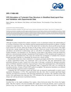
Fig. 1—Permeability field and well configuration for a sector model (Reservoir A).

simulation performance before and after the tuning procedure are then presented. We conclude with a discussion and a summary. Table 1—Six-component system for Reservoir Fluid A.

Our approach is based on a previous study (Fong et al. 1992), in which heuristic pressure/volume/temperature (PVT) characterization procedures were proposed to use two-phase fluid models to approximate the three hydrocarbon phases. Specifically, it is attempted to reduce/eliminate the three-phase region by adjusting the binaryinteraction coefficients (BICs) between CO2 and pseudocomponents. This was to match the upper curve of the V-L1-L2 region at high CO2 concentrations. The use of a two-phase model to represent the phase behavior of the three-phase region may significantly reduce the numerical instability with conventional two-hydrocarbon-phase simulators. In addition, the technique is independent of reservoir simulators, because the PVT recharacterization is performed with standalone PVT-simulation software. However, when the technique (Fong et al. 1992) was applied to our study, it was observed that the method cannot totally eliminate the three-phase region. Thus, numerical instability still existed in the flow simulation. In addition, the predicted saturation pressures were much lower than the measured data because the saturation points (V-L1 data) at low CO2 concentrations were not preserved when adjusting the BICs to match the upper boundary of the V-L1-L2 region. In this work, we propose a new PVT-modeling procedure. In our approach, it is the acentric factors of the pseudocomponents that are adjusted to eliminate the three-hydrocarbon-phase region. Then, the BICs between CO2 and pseudocomponents are tuned to match the saturation pressure (V-L1 data). Other parameters (of the pseudocomponents) are also adjusted to maintain other PVT measurements (such as the CO2 swelling test and MMP). It is shown that the acentric factors of the pseudocomponents have a strong impact on the three-phase region, and it is effective to adjust them to eliminate the three-phase region. To our knowledge, this was not studied in any of the previous investigations. The method is applied to two sector models from oil fields in west Texas (with fine-scale models of more than 600,000 gridblocks). For the cases considered, the new fluid characterization significantly improves the numerical stability (thus, reducing the simulation time), while having very little effect on the recovery predictions. The method is applicable to models with small threephase regions. For those cases, it represents an effective and practical solution for field-scale simulation of CO2 injection. This paper proceeds as follows. We first describe the problem encountered when simulating the CO2 injection at low temperatures. Then, the standard PVT characterization procedures for reservoir fluids are presented, including both PVT measurements and modeling. We then propose a tuning procedure to adjust the PVT parameters to eliminate the three-hydrocarbon-phase regions, while maintaining other important PVT properties. Numerical results to illustrate the

Problem Statement We first present an example to illustrate the numerical issue encountered in the simulation of CO2 injection at low temperatures. The example involves a sector model from an oil reservoir in west Texas (referred to as Reservoir A). The fine-scale model is of dimensions 28  28  777 ¼ 609,168; and the model resolution is dx ¼ dy  25 ft, and dz  1.5 ft (as shown in Fig. 1a). The fine-scale model is vertically coarsened (nonuniformly) to 200 layers and 100 layers, respectively (presented in Figs. 1b and 1c). One-quarter of a five-spot pattern is considered here—both the injector and the producer partially penetrate the reservoir. The reservoir temperature is 105 F. Table 1 presents the sixcomponent system for the initial reservoir fluid. The detailed pressure/volume/temperature (PVT) characterization is presented in the next sections. Pure CO2 is injected, and the minimum miscibility pressure (MMP) is approximately 1,250 psia. The well scheduling involves primary depletion, followed by water injection, then continuous gas injection, and then water-alternating-gas (WAG) injection. We consider various producer bottomhole pressures (BHPs), which lead to different reservoir pressures. Shown in Fig. 2 are the average reservoir pressure and centralprocessing-unit (CPU) time for the simulation of the upscaled 200-layer model, with two producer BHP values. Fig. 2a also displays the MMP ( ¼ 1,250 psi, the red line). We see that the simulation with producer BHP ¼ 1,070 psi gives an average reservoir pressure above MMP (therefore, referred to as a miscible displacement), whereas the average reservoir pressure with producer BHP ¼ 1,000 psi is slightly below the MMP (referred to as a nearmiscible displacement). However, the slight difference in the producer BHP (and thus, the reservoir pressure) leads to very different CPU time between the two simulation runs (displayed in Fig. 2b). We see that there is a dramatic increase of the simulation time with the near-miscible displacement (the black curve in Fig. 2b), indicating abnormal convergence behaviors in the simulation. This behavior also was observed in the simulations with the fine-scale model, the upscaled 100-layer model, and further-coarsened models. To investigate this problem, we also considered other producer BHPs (for further-coarsened models), and observed the abnormally increased simulation time even at the start of the continuous gas injection (i.e., immediately after the water injection). Thus, the problem occurs not only at the WAG injection. To further identify if the problem is CO2-specific, we changed the injection fluid from pure CO2 to a mixture of C1 (60 %mol) and C2–3 (40 %mol), which has a very similar MMP to CO2. For a wide range of producer BHPs (ranging from 750 to 1,100 psi), all the simulations ran smoothly. This indicates that the problem is likely caused by CO2-related issues. Detailed debugging showed that, for many timesteps, there were oscillations in pressure, saturation, and phase-composition

May 2015 SPE Reservoir Evaluation & Engineering ID: jaganm Time: 21:16 I Path: S:/3B2/REE#/Vol00000/150008/APPFile/SA-REE#150008

251

Stage:

1,800

12,500

1,600

10,000 Miscible displacement (producer BHP = 1,070 psi)

1,400

MMP = 1,250 psi

1,200

Near-miscible displacement (producer BHP = 1,000 psi)

1,000 800

0 PD

5,000 WI

10,000 15,000 20,000 Time (days) GI WAG

25,000

(a) Average reservoir pressure

PFTCPU (seconds)

Average Pressure (psia)

REE170903 DOI: 10.2118/170903-PA Date: 13-May-15

Page: 252

Total Pages: 14

Near-miscible displacement

7,500 5,000 Miscible displacement

2,500 0

PD

0

5,000

WI

1,000 15,000 Time (days)

GI

20,000

25,000

WAG

(b) CPU time (16 processors)

Fig. 2—Average reservoir pressure and CPU time for miscible (producer BHP 5 1,070 psi) and near-miscible (producer BHP 5 1,000 psi) displacements (Reservoir A, upscaled 200-layer model). The near-miscible displacement shows significantly increased simulation time.

(referred to as Reservoir B). The reservoir temperature is 110 F, and the reservoir fluid composition is listed in Table 2.

Table 2—Composition of Reservoir Fluid B.

changes from the flash calculation and Newton iteration. Previous studies (e.g., Khan et al. 1992; Okuno et al. 2010; Lins et al. 2011) reported similar observations. The problem may be caused by the discontinuous change in physical properties (e.g., phase density), because there is more than one two-phase solution. From our experience, the most likely two-phase solutions are oil/gas and oil/CO2-rich-liquid phases. We then performed standalone flash calculations with a PVT package. It confirmed the existence of the three hydrocarbon phases at similar conditions. This motivates us to develop a PVT recharacterization procedure to eliminate the three-phase region, while sufficiently approximating the fluid PVT properties.

Pressure/Volume/Temperature (PVT) Characterization of Reservoir Fluid We start our discussion with standard procedures to characterize reservoir fluids. The PVT characterization of a reservoir fluid is to provide necessary parameters for the determination of the thermodynamic and physical properties of the reservoir fluid. For a given reservoir fluid, a series of PVT measurements are first conducted to determine the experimental status/value of the phase behavior and physical properties. Those measured data are then used to tune and verify the equation-of-state (EOS) parameters through PVT modeling. In this section, the PVT measurements and modeling procedures are illustrated with another field from west Texas

PVT Measurements. The standard PVT tests to measure densities, viscosities, saturation points, and other properties of a reservoir fluid often include separator tests, constant-compositionexpansion (CCE) tests, CO2 swelling tests, and slimtube tests. Creek and Sheffield (1993) presented detailed experimental measurements of two reservoir samples from west Texas fields. For the details of those standard PVT measurements, please also refer to Danesh (1998) and Pedersen et al. (1989). Summarized in Table 3 are some measured properties of Reservoir Fluid B. The results from CCE tests (such as oil density and viscosity) are shown in Fig. 3 (the red curves, along with the PVT modeling results to be discussed later). In Fig. 3c, the relative volume is defined by a total volume normalized by the volume at the bubblepoint. The results from CO2 swelling tests, in which a given amount of reservoir fluid is mixed with CO2 progressively, are displayed in Figs. 4 and 5. The measured saturation pressure is shown in Fig. 4 (again along with the PVT modeling results). Also displayed in Fig. 4 is a three-hydrocarbon-phase region (to be discussed later). The measured relative volumes at the different CO2 concentrations are presented in Fig. 5 (the red curves). The minimum miscibility pressure (MMP) is obtained by a series of slimtube tests with pressure varying from immiscible to miscible displacements. For Reservoir B, the measured MMP from slimtube tests is 1,250 psia at 110 F. Modeling of PVT Experiments. With the experimental data obtained previously, we now consider the modeling of the PVT measurements. In this work, modified Peng-Robinson EOS (Robinson and Peng 1978) is applied for the PVT modeling, and the Lohrenz et al. (1964) (LBC) viscosity model is used for viscosity estimation for both the vapor and liquid phases. The reservoir fluid is first characterized into several components, and then the parameters of EOS and the viscosity model are tuned with the experimental data. A stand-alone PVT simulation package is applied here for the purpose. Specifically, Reservoir Fluid B is characterized into a six-component system (see Table 4), and the standard PVT modeling procedure is briefly described next: 1. Split the C7þ fraction of the fluid into two pseudocomponents (i.e., C12 and C35 in Table 4) with a semicontinuous thermodynamic theory.

Table 3—Summary of measured properties for Reservoir Fluid B. 252

May 2015 SPE Reservoir Evaluation & Engineering ID: jaganm Time: 21:17 I Path: S:/3B2/REE#/Vol00000/150008/APPFile/SA-REE#150008

REE170903 DOI: 10.2118/170903-PA Date: 13-May-15

4

49

Experimental Modeled (standard)

47

Modeled (standard)

Modeled (standard)

3

1.400 1.200

2 1.000 1

1,200 1,600 Pressure (psia)

Experimental

1.600 V/Vb

51

Total Pages: 14

1.800 Experimental

53

45 800

Page: 253

5

viscosity (cp)

Density (lbm/ft3)

55

Stage:

0

2,000

500

1,000

1,500

0.800

2,000

0

Pressure (psia)

(a) Oil density

500

1,000 1,500

2,000

Pressure (psia) (c) Relative volume

(b) Oil viscosity

Fig. 3—Comparison of experimental measurements and PVT-modeling results (standard PVT characterization) for Reservoir Fluid B.

1,450

L1–L2

1,350 L1

1,250

Pressure (psia)

1,150

L1–L2–V

1,050 L1–V

950 850

Three-phase upper boundary 750

Three-phase lower boundary

650

Saturated pressure calculated

550

Saturated pressure measured

450 0

20

80

40 60 CO2% (mole) in oil/CO2 mixture

Fig. 4—P-x diagram for the Reservoir Fluid B/CO2 mixtures with standard PVT characterization.

3

2.5

3 Experimental

2.5

Modeled (standard)

Modeled (standard)

V/Vb

2 1.5

Experimental

Experimental

2

Modeled (standard)

2 V/Vb

2.5 V/Vb

2. Combine defined components (i.e., N2þC1, H2SþC2þC3, and C4þC5þC6). 3. Adjust the binary-interaction coefficients (BICs, kij) of C1pseudocomponents to match oil-bubblepoint pressure. 4. Adjust the volume-shift parameter (S) of pseudocomponents to match oil densities. 5. Adjust the critical volume (Vc in the LBC viscosity model) of pseudocomponents to match oil viscosities. 6. Adjust the BICs of CO2-pseudocomponents to match saturation pressures in the CO2 swelling test (i.e., V-L1 data). 7. Check the total gas/oil ratio (GOR), stock-tank-oil density, and formation volume factor (FVF) at bubblepoint pressure with the measured data for the reservoir fluid. 8. Check the PVT prediction of the CCE test with measured data for the reservoir fluid and the CO2/oil mixtures. 9. Perform simulations of 1D slimtube displacements to obtain an estimated MMP, and compare it with measured data. The characterization results are shown in Table 4, in which the six components and their associated PVT parameters are listed. Table 5 presents the BICs among those components.

1.5

1.5 1 0.5 200

1 400

600 800 Pressure (psia)

1,000

(a) 28.4% (mole) CO2 in CO2/oil mixture

0.5 500

700 900 Pressure (psia)

1 600

1,100

(b) 47.2% (mole) CO2 in CO2/oil mixture

800 1,000 1,200 1,400 Pressure (psia)

(c) 60.5% (mole) CO2 in CO2/oil mixture

Fig. 5—Comparison of experimental measurements and PVT-modeling results (standard PVT characterization) for CCE test of Reservoir Fluid B/CO2 mixtures.

Table 4—PVT parameters from standard characterization for Reservoir Fluid B. May 2015 SPE Reservoir Evaluation & Engineering ID: jaganm Time: 21:17 I Path: S:/3B2/REE#/Vol00000/150008/APPFile/SA-REE#150008

253

REE170903 DOI: 10.2118/170903-PA Date: 13-May-15

Table 5—BICs from standard characterization for Reservoir Fluid B.

With the characterization described previously, we now compare the modeled and measured fluid properties and other PVT data. Table 6 presents the comparison of the measured and modeled fluid properties, including total GOR, oil density, and FVF. We see that the data from the PVT modeling are very close to the experimentally measured data. Other results from the CCE test for the reservoir fluid are shown in Fig. 3, in which the oil density, oil viscosity, and relative volume are displayed. The results from PVT modeling (blue dots) match the experimental results (red curves) well. Next are the results from the CO2 swelling test, as shown in Fig. 4. In the P-x diagram, the green curve represents the modeled saturation pressures, which matches the measured data well. In Fig. 4, there is a small three-hydrocarbon-phase region (labeled as L1-L2-V), with the CO2 concentration between 65 and 85%, and the pressure ranging from 1,250 to 1,330 psia (note that the MMP is approximately 1,250 psia). This small three-phase region was also observed in the experiments. As discussed earlier, the threephase region may cause numerical instability with conventional two-hydrocarbon-phase simulators. Shown in Fig. 5 are the results of the CCE test for the oil/CO2 mixtures. The red curves represent the experimental data, and the blue dots depict the PVT modeling results. For all the CO2 concentrations (28.4, 47.2, and 60.5%), the PVT characterization represents the experimental data well. Note that the PVT characterization procedure described here represents “Procedure A” in the study of Fong et al. (1992). One can view the procedure as a standard fluid characterization, in which the V-L1 (saturation point) data are matched by tuning the BICs between the CO2 and pseudocomponents. With this approach, for reservoir-fluid/CO2 mixtures at low temperatures, three-hydrocarbon-phase regions may exist (as seen here). Next, we present our approach to adjust the PVT characterization to eliminate the three-phase region. Pressure/Volume/Temperature (PVT) Modeling Procedure To Eliminate Three-Phase Region Fong et al. (1992) presented a study to reduce/eliminate threehydrocarbon-phase regions by adjusting the binary-interaction coefficients (BICs) between the CO2 and pseudocomponents to match the upper boundary of the V-L1-L2 data (blue curve in Fig. 4). As discussed in the Introduction, when the method was applied

Stage:

Page: 254

Total Pages: 14

in this work, it was unable to remove the three-phase region completely, and numerical instability was still observed. Note that a pseudocomponent is an aggregation of many components, and its thermodynamic properties (Tc, Pc, x), as well as BICs with other components, are adjustable. Other studies considered the adjustments of the critical properties (Tc, Pc) of the pseudocomponents to eliminate the three-phase region. However, we again found the method was not effective. In our study, it was observed that the acentric factor x has a much stronger effect on the phase behavior than Tc and Pc. We found that the three-phase region is sensitive to the x value of pseudocomponents, and the appropriate tuning of the x values can effectively eliminate the three-phase region. Tuning Procedure. Our proposed approach consists of two steps. First, we adjust the acentric factor (x) of pseudocomponents to eliminate the three-hydrocarbon-phase region. Then, other PVT parameters (of pseudocomponents) are tuned further to match the saturation pressures and other PVT measurements. Specifically, the tuning procedure includes the following steps:  Adjust the value of the acentric factor x for each pseudocomponent until the three-hydrocarbon-phase region disappears in the P-x diagram of the crude/CO2 mixtures. For Reservoir Fluid B (which includes two pseudocomponents, C12 and C35), the increase of x for the lighter pseudocomponent (C12), and/or the decrease of x for the heavier one (C35), leads to the shrinking of the three-phase region, and eventually eliminates the three-phase region. For our test samples, the effective range of x is approximately a 20 to 30% increase of x for C12, and a 10 to 15% decrease of x for C35. The impact of x on the three-phase region is discussed in more detail later. • Adjust the BICs of CO2-pseudocomponent to match the saturation pressures in the CO2 swelling test (V-L1 data). • Adjust the BICs of C1-pseudocomponent to match oil bubblepoint pressure. • Repeat Steps 4, 5, 7, 8, and 9 in the standard characterization procedure described earlier to match other PVT data, such as oil density, oil viscosity, results from CCE tests, and minimum miscibility pressure (MMP) estimation. With the new PVT characterization procedure described previously, the adjusted PVT parameters and BICs of the pseudocomponents (C12 and C35) are presented in Tables 7 and 8. Compared with those obtained from the original/standard characterization (Tables 4 and 5), the x value increased from 0.504 to 0.63 for the lighter pseudocomponent (C12), whereas the x value for the heavier pseudocomponent (C35) decreased from 1.179 to 0.955. Note that, for this case (Reservoir Fluid B), because the CO2 concentration is small (1.35%, mole) in the initial reservoir fluid, the critical volume (Vc) and volume-shift parameter (S) of the pseudocomponents do not need to be adjusted further to match the viscosity and density measurements. Shown in Fig. 6 is the P-x diagram for Reservoir Fluid B, with the new PVT characterization. Compared with the original P-x

Table 6—Comparison of measured and modeled (standard characterization) fluid properties for Reservoir Fluid B.

Table 7—Parameters adjusted in the new characterization for Reservoir Fluid B. 254

Table 8—BICs adjusted in the new characterization for Reservoir Fluid B. May 2015 SPE Reservoir Evaluation & Engineering

ID: jaganm Time: 21:17 I Path: S:/3B2/REE#/Vol00000/150008/APPFile/SA-REE#150008

REE170903 DOI: 10.2118/170903-PA Date: 13-May-15

Experimental

Pressure (psia)

2,000 Modeled (adjusted) 1,500

1,000

500

0 40

20

Page: 255

Total Pages: 14

still match well. Note that, in Fig. 6, there is a steep increase of the modeled saturation pressure at high CO2 concentrations. This represents the boundary between the L1 (oil-rich liquid) region and the L1–L2 (oil-rich and CO2-rich liquid) region, which is supported by experimental data and well-documented in the literature (e.g., Fong et al. 1992; Creek and Sheffield 1993). Next, we will compare other fluid properties (modeled with the new PVT characterization) with the PVT experiments.

2,500

0

Stage:

60

80

CO2% (mole) Fig. 6—P-x diagram for Reservoir Fluid B/CO2 mixtures with new characterization.

diagram obtained from the standard PVT characterization (Fig. 4), the three-hydrocarbon-phase region disappears, showing that the proposed method serves the purpose to eliminate the threephase region. Also of interest is the comparison of the modeled saturation pressure (green curve) and the experimental data—they

Comparison With PVT Experiments. Shown in Table 9 are the comparisons of the total gas/oil ratio, formation volume factor at bubblepoint, and the stock-tank-oil density. The new model is comparable to the original characterization (Table 6). Both match the experimental data well. Fig. 7 presents the comparisons of oil density, oil viscosity, and relative volume obtained from a constant-composition-expansion (CCE) test for the reservoir fluid. Displayed in Fig. 8 are the relative volumes from CCE tests for the CO2/oil mixtures at different CO2 concentrations. All these results show a good agreement between the modeled and measured data, showing comparable accuracy with the original PVT characterization (Figs. 3 and 5). With the new PVT characterization, we also simulate slimtube displacements to estimate MMP. The predicted MMP is 1,300 psia, close to the measured value (1,250 psia). Note that, in our study, it was observed that, although the adjustments of x values for the pseudocomponents have a strong impact on the three-phase region, they had little effect on the other PVT properties. Further, in the proposed procedure, we

Table 9—Comparison of measured and modeled (new characterization) fluid properties for Reservoir Fluid B.

1.800

5 Experimental

53

4

49

Experimental Modeled (standard)

47 45 800

Modeled (standard)

Modeled (standard)

3

1.400 1.200

2 1.000 1

1,200 1,600 Pressure (psia)

Experimental

1.600 V/Vb

51

viscosity (cp)

Density (lbm/ft3)

55

0

2,000

500

1,000

1,500

0.800

2,000

Pressure (psia)

(a) Oil density

0

500

1,000 1,500

2,000

Pressure (psia) (c) Relative volume

(b) Oil viscosity

Fig. 7—Comparison of experimental measurements and PVT modeling results (new PVT characterization) for Reservoir Fluid B. 3 Experimental

2.5

Modeled (adjusted)

Modeled (adjusted)

V/Vb

2 1.5

Experimental

Experimental

2

Modeled (adjusted)

2 V/Vb

2.5 V/Vb

2.5

3

1.5

1.5 1 0.5 200

1 400

600 800 Pressure (psia)

1,000

(a) 28.4% (mole) CO2 in CO2/oil mixture

0.5 500

700 900 Pressure (psia)

1,100

(b) 47.2% (mole) CO2 in CO2/oil mixture

1 600

800 1,000 1,200 1,400 1,600 Pressure (psia)

(c) 60.5% (mole) CO2 in CO2/oil mixture

Fig. 8—Comparison of experimental measurements and PVT-modeling results (new PVT characterization) for CCE test of Reservoir Fluid B/CO2 mixtures. May 2015 SPE Reservoir Evaluation & Engineering ID: jaganm Time: 21:17 I Path: S:/3B2/REE#/Vol00000/150008/APPFile/SA-REE#150008

255

REE170903 DOI: 10.2118/170903-PA Date: 13-May-15

Upper: ω12 = 0.5040 Lower: ω12 = 0.5040 Upper: ω12 = 0.5166 Lower: ω12 = 0.5166 Upper: ω12 = 0.5292 Lower: ω12 = 0.5292 Upper: ω12 = 0.4788 Lower: ω12 = 0.4788

1,330

Pressure (psia)

1,320 1,310 1,300 1,290 1,280 1,270

Upper: ω35 = 1.1201

1,310

Lower: ω35 = 1.1201

1,300

Upper: ω35 = 1.2380

1,290

Lower: ω35 = 1.2380

1,280 1,270

1,250

1,250

1,240 60

1,240 60

75

80

85

90

CO2% (mole) in Oil/CO2 Mixture

Upper: ω35 = 1.179 Lower: ω35 = 1.179

1,320

1,260

70

Total Pages: 14

1,330

1,260

65

Page: 256

1,340

Pressure (psia)

1,340

Stage:

65

70 75 80 CO2% (mole) in Oil/CO2 Mixture

85

Fig. 9—Effect of xC12 on three-phase region (original: 0.5040) for Fluid B/CO2 mixtures.

Fig. 10—Effect of xC35 on three-phase region (original: 1.1790) for Fluid B/CO2 mixtures.

adjusted the BICs of CO2-pseudocomponents (see Table 8) to match the saturation pressures (as shown in Fig. 6), and repeated several steps in the standard characterization to ensure that the new characterization matches other PVT properties.

ference in the reservoir fluid (see Table 4). We note that the concentrations of the two pseudocomponents are quite different: 40% (mole) for C12 vs. 14% for C35. Therefore, the value of xC12 has a stronger effect on the three-phase region than the value of xC35. One should keep in mind that the results shown in Figs. 9 and 10 represent only the mixtures of the initial reservoir fluid and CO2. During the flow simulation, the fluid composition in a given gridblock can change dramatically from the initial fluid. Thus, the values of xC12 and xC35 are adjusted to a wider range than those shown in Figs. 9 and 10. This is to ensure better stability in the flow simulation. For this reservoir fluid, the values of xC12 ¼ 0.63 and xC35 ¼ 0.955 (compared with the original values: xC12 ¼ 0.504 and xC35 ¼ 1.179) are used in the flow simulation.

Impact of x on Three-Phase Region. We now present the results for the impact of x on the three-phase region. First, we keep the value of xC35 as the original one (1.1790), and vary the value of xC12. Fig. 9 plots the three-phase region corresponding to four different values of xC12—the original value 0.504, the value with 2.5% increase (0.5166), the value with 5% increase (0.5292), and the value with 5% decrease (0.4788). As shown in Fig. 9, the slight increase (2.5%) of xC12 significantly shrinks the three-phase region (green curves), and the 5% increase reduces further the three-phase region to very small (blue curves) (i.e., CO2% ranges 70 to 77%, and pressure ranges 1,274 to 1,302 psia). In fact, the three-phase region does not exist anymore if the value of xC12 increases by 10% to 0.5544. On the other hand, the decrease of xC12 gives the opposite effect—we see that, if xC12 decreases by 5% to 0.4788, the three-phase region (black curves in Fig. 9) becomes even larger than the original three-phase region (red curves). Next, we change the x value for the heavier pseudocomponent xC35, and keep the lighter pseudocomponent xC12 as the original value (0.504). The results are shown in Fig. 10. The original value of xC35 is 1.179, giving the three-phase region shown in Fig. 10 (the red curves). When the value of xC35 decreases by 5% to 1.1201, the three-phase region shrinks significantly (the green curves). By contrast, if we increase the value of xC35 by 5% to 1.2380, the three-phase region increases considerably (the yellow curves). It is observed that, although the three-phase region shrinks with the decrease of the value of xC35, it is very hard to eliminate the three-phase region by only reducing the value of xC35. Instead, the 10% increase of xC12 can effectively eliminate the three-phase region. This may be caused by the compositional dif-

Characterization of Reservoir Fluid for Reservoir A. Before we present the simulation results, we briefly describe the characterization for Reservoir Fluid A (which was considered in the Problem Statement section). Recall that Reservoir A is also an oil reservoir from west Texas with a reservoir temperature of 105 F. Table 10 presents the original PVT characterization from the standard procedure—the reservoir fluid is represented by a sixcomponent system, including two pseudocomponents (C11 and C31). Table 11 lists the BICs from the original characterization. Although there is no three-hydrocarbon-phase region observed in the initial reservoir fluid/CO2 mixtures, the three-phase (V-L1-L2) region did occur during the flow simulation, which caused the severe numerical instability shown in Fig. 2b (as discussed in the Problem Statement section). To overcome the numerical instability encountered, we output the reservoir fluid from the simulation (at timesteps when the three-phase region most likely occurs), and apply the new PVT characterization procedure to the mixture of that reservoir fluid and CO2. Tables 12 and 13 present the new PVT parameters. We see that the x value for the lighter pseudocomponent (xC11) increases from 0.444 (the original value) to 0.544, whereas the one for the heavier pseudocomponent (xC31) decreases from 1.0339 to 0.850. For this case, the critical volume (Vc) and volume-shift

Table 10—Properties from standard PVT characterization for Reservoir Fluid A. 256

May 2015 SPE Reservoir Evaluation & Engineering ID: jaganm Time: 21:17 I Path: S:/3B2/REE#/Vol00000/150008/APPFile/SA-REE#150008

REE170903 DOI: 10.2118/170903-PA Date: 13-May-15

Stage:

Page: 257

Total Pages: 14

Table 12—Parameters adjusted from new characterization for Reservoir Fluid A. Table 11—BICs from standard characterization of Reservoir Fluid A.

1,600

Table 13—BICs adjusted from new characterization for Reservoir Fluid A.

Pressure (psia)

Experimental Modeled (standard)

1,350

Modeled (adjusted)

1,100 850

PFTCPU (seconds)

12,500

600

BHP = 1,000 psia BHP = 1,100 psia

10,000

0

40

60

CO2% (mole)

7,500 5,000

Near-miscible displacement

2,500

Miscible displacement

0

20

0

PD

5,000 WI

10,000 15,000 Time (days) GI

20,000

25,000

WAG

Fig. 12—CPU time with new PVT characterization for the miscible and near-miscible displacements (Reservoir A, upscaled 200-layer model, producer BHPs 5 1,100 psia and 1,000 psia, respectively).

parameter (S) are also adjusted to match other PVT measurements (e.g., oil density and oil viscosity). Similarly, to match the saturation pressures in the CO2-swelling test, the BICs of CO2-pseudocomponent are also adjusted (as shown in Table 13). We also compared the new PVT characterization with the measured PVT data for Reservoir Fluid A. The adjustment of PVT parameters (shown in Tables 12 and 13) eliminates the three-phase region encountered in the flow simulation, while still matching well the fluid properties from the PVT measurements. As an example, the comparison of saturation pressure between the experimental data and the new characterization (as well as the standard characterization) is shown in Fig. 11. In addition, the simulated MMP (from slimtube displacements) is 1,250 psia, which matches the measured MMP value (1,250 psia). Simulation Results Next, we present simulation results to illustrate the efficiency of the proposed pressure/volume/temperature (PVT) recharacterization procedure. All the flow simulations are performed with a next-generation reservoir simulator. The simulator shows excellent performance in two-phase equilibrium calculations (with reduced variables and bypassing method; e.g., Pan and Tchelepi 2011), multistage linear solver, and scalable parallel capabilities. Although the adaptive implicit method is available in the formula-

Fig. 11—P-x diagram for Reservoir Fluid A/CO2 mixtures with standard and new characterizations.

tion, the full implicit method is considered here for all the simulations. Parallel simulations with 32 processors in a Linux cluster are applied to the fine-scale models, whereas simulations with 16 processors are considered for the coarse-scale models. Simulation Results for Reservoir A. The first example was introduced in the Problem Statement section. Please refer to that section for the details about the reservoir model and problem setup. Here, we compare the simulation results between the original PVT characterization and the new procedure (which eliminates the three-hydrocarbon-phase region). The simulation results are presented from two aspects: simulation performance (i.e., CPU time) and recovery predictions. Comparison of Simulation Time. As discussed earlier, the simulation of the near-miscible displacement for the upscaled 200-layer model (the black curve in Fig. 2b) shows significantly increased simulation time, indicating numerical instability in the simulation. We then applied the new PVT recharacterization to eliminate the three-hydrocarbon-phase region. The results of the CPU time for both the miscible and near-miscible displacements are shown in Fig. 12. In contrast to the original fluid characterization (Fig. 2b), the CPU time for the near-miscible displacement reduces substantially (the black curve in Fig. 12), indicating that the simulation now converges normally. More results are shown in Table 14, which summarizes the CPU time with the original and new PVT characterizations for the near-miscible displacements, with different model sizes (the upscaled 100- and 200-layer models, and the fine-scale 777-layer model). For the fine-scale model, the CPU time with the original characterization takes approximately 40 hours (with 32 processors), whereas the simulation with the new characterization takes only approximately 21=2 hours. The tremendous reduction of CPU time is also observed for the upscaled models.

Table 14—Comparison of CPU time between the original and new characterizations (Reservoir A, producer BHP 5 1,000 psia). May 2015 SPE Reservoir Evaluation & Engineering ID: jaganm Time: 21:17 I Path: S:/3B2/REE#/Vol00000/150008/APPFile/SA-REE#150008

257

600

600,000

500

500,000

Cum-Oil Prod (STB)

Oil-Prod Rate (STB/day)

REE170903 DOI: 10.2118/170903-PA Date: 13-May-15

Original PVT New PVT (adjusted ω)

400 300 200 100 0 0

5,000

10,000

15,000

20,000

Original PVT New PVT (adjusted ω)

200,000 100,000 5,000

10,000

15,000

20,000

25,000

Time (days)

(a) Oil-Production Rate

(b) Cumulative-Oil Production 600,000

500 400

Cum-Oil Prod (STB)

Gas-Prod Rate (MSCF/day)

Total Pages: 14

300,000

Time (days)

Original PVT New PVT (adjusted ω)

300 200 100 0 0

Page: 258

400,000

0 0

25,000

Stage:

5,000

10,000

15,000

20,000

25,000

Time (days)

(c) Gas-Production Rate

500,000 Original PVT New PVT (adjusted ω)

400,000 300,000 200,000 100,000 0 0

5,000

10,000

15,000

20,000

25,000

Time (days)

(d) Cumulative-Gas Production

Fig. 13—Comparison of recovery prediction with original and new PVT characterizations (Reservoir A, fine-scale 777-layer model, producer BHP 5 1,000 psia).

Comparison of Recovery Predictions. We next compare the recovery predictions between the original and the new PVT characterizations. The first set of results involves the fine-scale 777layer model. Displayed in Fig. 13 are the comparisons of oil and gas productions with the original and new fluid characterizations for the near-miscible displacements. With the original characterization, the oil- and gas-production rates (Figs. 13a and 13c) show severe instability (oscillation), which explains the very long CPU time (more than 40 hours) for the simulation run. The simulation with the new PVT characterization, by contrast, runs very smoothly (with CPU time reduced to 21=2 hours). For the cumulative production (oil and gas), the new and original characterizations present close predictions, although there is some discrepancy in the cumulative gas production, which may be caused by the numerical instability with the original characterization. Similar observations also apply to the results for the upscaled models. Shown in Fig. 14 are the results for the near-miscible displacement for the upscaled 100-layer model. Similarly, the original fluid characterization gives significantly increased simulation time (although there are no obvious oscillations observed in the oil- and gas-production rates for this case). Again, for the oil production, the prediction with the new characterization shows very close agreement with the original one. For the gas production, however, there is a difference starting at the gas-breakthrough time (shown in Figs. 14c and 14d). As explained earlier, the difference here may be caused by the numerical instability inherent with the original fluid properties. In addition to the previous results for the near-miscible displacement, we also present the recovery predictions of the miscible displacement (for the upscaled 100-layer model, as shown in Fig. 15). Recall that, for this case, the simulation ran smoothly even with the original PVT characterizations (illustrated by the orange curve in Fig. 2b). Therefore, the original results can be viewed as reliable predictions. Fig. 15 shows that the original and new fluid characterizations provide very close recovery predictions for both the oil and gas productions. Note that the PVT recharacterization procedure does change the PVT parameters (to 258

eliminate the three-phase region). However, because the key fluid properties are maintained (also by tuning the PVT parameters), the recovery predictions are very close. In our study, we compared the simulation results between the original and new PVT characterizations for a variety of producer bottomhole pressures (BHPs), ranging from 600 to 1,400 psia (with an interval of 100 psia). A very close agreement in the recovery predictions was observed for almost all the cases, except the slight difference in the gas production for producer BHP ¼ 1,000 psia (as shown in Figs. 13 and 14 and discussed previously). Simulation Results for Reservoir B. We next present the simulation results for Reservoir B. For this model, the detailed PVT characterizations (original and new) were presented in the previous sections to illustrate the recharacterization procedure. Fig. 16a displays the fine-scale sector model, with dimensions 43  44  300 ¼ 567,600, and model resolution dx ¼ dy  50 ft, dz  1.0 ft. A coarse-scale model is generated by vertically (and nonuniformly) coarsening the model to 55 layers. Shown in Fig. 16b are the low-permeability (500 md) regions in the model. The high-permeability layers (red in Fig. 16b) make the simulation challenging for this case. One-quarter of a five-spot pattern is considered here, with the injector at (5, 5, 1), and the producer at (38, 39, 1). Both wells partially penetrate the reservoir. The well scheduling again starts with primary depletion (until 1,000 days), followed by water injection (until 3,000 days), and continuous CO2 injection (until 6,200 days), and finally water-alternating-gas injection to 15,000 days. Performance for Upscaled Model. We again consider various producer BHPs (ranging from 800 to 1,300 psia, with an interval of 100 psia). These will lead to different reservoir pressures. For this reservoir fluid, the initial reservoir fluid and CO2 mixtures present a small three-phase region with the original fluid characterization (as shown in Fig. 4). Therefore, one may encounter numerical issues. Table 15 summarizes the CPU time between the original and new PVT characterizations for the various producer May 2015 SPE Reservoir Evaluation & Engineering

ID: jaganm Time: 21:17 I Path: S:/3B2/REE#/Vol00000/150008/APPFile/SA-REE#150008

REE170903 DOI: 10.2118/170903-PA Date: 13-May-15

Stage:

300 Original PVT New PVT (adjusted ω)

200 100

5,000

10,000

15,000

20,000

500,000

Cum-Oil Prod (STB)

Oil-Prod Rate (STB/day)

400

400,000 300,000 Original PVT New PVT (adjusted ω)

200,000 100,000 0 0

25,000

5,000

15,000

20,000

25,000

(b) Cumulative-Oil Production

(a) Oil-Production Rate 500,000 Cum-Oil Prod (STB)

250 Gas-Prod Rate (MSCF/day)

10,000

Time (days)

Time (days)

200 Original PVT New PVT (adjusted ω)

150 100 50 0

Total Pages: 14

600,000

500

0 0

Page: 259

400,000

200,000 100,000 0

0

5,000

10,000

15,000

20,000

Original PVT New PVT (adjusted ω)

300,000

25,000

0

5,000

10,000

15,000

20,000

25,000

Time (days)

Time (days)

(d) Cumulative-Gas Production

(c) Gas-Production Rate

Fig. 14—Comparison of recovery prediction with original and new PVT characterizations (Reservoir A, upscaled 100-layer model, producer BHP 5 1,000 psia).

zation also reduced the simulation time for the two cases in which the original characterization ran through (i.e., producer BHP ¼ 800, 900 psia). To verify the recovery predictions with the new fluid characterization, we now compare the simulation results between the

500

600,000

400

500,000

300 Original PVT New PVT (adjusted ω)

200 100 0

0

5,000

10,000

15,000

20,000

Cum-Oil Prod (STB)

Oil-Prod Rate (STB/day)

BHPs. For the original fluid characterization, all the simulations with producer BHP >900 psia failed to converge. The new fluid characterization eliminates the three-phase region (as displayed in Fig. 6). As a result, all the simulations with the various producer BHPs ran through with normal convergence. The new characteri-

400,000 300,000

100,000 0

25,000

Original PVT New PVT (adjusted ω)

200,000

0

5,000

Time (days)

200

400,000

Cum-Oil Prod (STB)

Gas-Prod Rate (MSCF/day)

500,000

150 Original PVT New PVT (adjusted ω)

50

5,000

10,000

15,000

20,000

25,000

(b) Cumulative-Oil Production

(a) Oil-Production Rate

0 0

15,000

Time (days)

250

100

10,000

20,000

Time (days)

(c) Gas-Production Rate

25,000

300,000

Original PVT New PVT (adjusted ω)

200,000 100,000 0

0

5,000

10,000

15,000

20,000

25,000

Time (days)

(d) Cumulative-Gas Production

Fig. 15—Comparison of recovery prediction with original and new PVT characterizations (Reservoir A, upscaled 100-layer model, producer BHP 5 1,100 psia). May 2015 SPE Reservoir Evaluation & Engineering ID: jaganm Time: 21:17 I Path: S:/3B2/REE#/Vol00000/150008/APPFile/SA-REE#150008

259

REE170903 DOI: 10.2118/170903-PA Date: 13-May-15

(a) Permeability field

Stage:

Page: 260

Total Pages: 14

(b) Low-permeability (500 md, red) Fig. 16—Fine-scale permeability field for Reservoir B.

Table 15—Comparison of CPU time between original and new characterizations for Reservoir Fluid B (upscaled model, 16 processors).

Table 16—Comparison of CPU time between original and new PVT characterizations for Reservoir Fluid B (fine-scale model, 32 processors).

original and the new fluid characterizations. Fig. 17 presents the results for producer BHP ¼ 900 psia. This is the highest producer BHP in which the simulation with the original fluid characterization converged. The results in Fig. 17 display a very close agreement (oil, gas, and CO2 production rates) between the original and new fluid characterizations, consistent with the results shown earlier for Reservoir A. For this case, by comparing the averaged reservoir pressure and minimum miscibility pressure, we see that we can view the simulation as an immiscible displacement. Because none of the simulations (for the original fluid characterization with producer BHP above 900 psia) provided converged results, it is impossible

to compare the recovery predictions for cases with higher reservoir pressures. Nonetheless, the CPU time shown in Table 15 is convincing that the simulations with the new PVT characterization do converge normally. Performance for Fine-Scale Model. We next present the results for the fine-scale model, with dimensions 43  44  300 ¼ 567,600. Table 16 shows the comparison of CPU time between the original and the new fluid characterizations for various producer BHPs. With the new characterization, all the simulations ran through—it took approximately 3 to 5 hours to complete the runs for the fine-scale model. The simulations with the original characterization, by contrast, failed to converge, or Gas-Prod Rate (MSCF/day)

Oil-Prod Rate (STB/day)

2,500 2,000 Original PVT New PVT (adjusted ω)

1,500 1,000 500 0 0

2,500

5,000

10,000 7,500 Time (days)

12,500

15,000

500 400 Original PVT New PVT (adjusted ω)

300 200 100 0

0

2,500

(a) Oil-Production Rate

5,000

7,500 10,000 Time (days)

12,500

15,000

(b) Gas-Production Rate

ZPRCO2 (LB-M/D) (MSCF/day)

100 80

Original PVT New PVT (adjusted ω)

60 40 20 0 0

2,500

5,000

7,500 10,000 Time (days)

12,500

15,000

(c) CO2 Production Rate Fig. 17—Comparison of recovery prediction and CO2 production rates with original and new PVT characterizations (Reservoir B, upscaled model, BHP 5 900 psia). 260

May 2015 SPE Reservoir Evaluation & Engineering ID: jaganm Time: 21:17 I Path: S:/3B2/REE#/Vol00000/150008/APPFile/SA-REE#150008

REE170903 DOI: 10.2118/170903-PA Date: 13-May-15

Stage:

Total Pages: 14

400,000 Original PVT New PVT (adjusted ω)

2,000 1,500 1,000 500 0 0

2,500

5,000

7,500 10,000 Time (days)

12,500

Cum-Gas Prod(MSCF)

2,500 Oil-Prod Rate (STB/day)

Page: 261

320,000 240,000 Original PVT New PVT (adjusted ω)

160,000 80,000 0 0

15,000

2,500

5,000

7,500 10,000 Time (days)

12,500

15,000

(b) Cumulative-Gas Production

(a) Oil-Production Rate

ZPRCO2 (LB-M/D)

100 80

Original PVT New PVT (adjusted ω)

60 40 20 0 0

2,500

5,000

7,500 10,000 Time (days)

12,500

15,000

(c) CO2 Production Rate Fig. 18—Comparison of recovery prediction and CO2 production rates with original and new PVT characterizations (Reservoir B, fine-scale model, producer BHP 5 900 psia).

took much longer time (20 to 40 hours) for the two cases with producer BHP ¼ 800 and 900 psia. The comparisons of recovery predictions are presented in Fig. 18—again for one of the cases in which the simulation with the original fluid characterization did run through (i.e., producer BHP ¼ 900 psia). Similar to the results for the upscaled model (shown earlier), the two sets of results here also present very close recovery predictions with the original and new characterizations. For the cases considered, it is shown that the new characterization leads to more-stable simulations (thus, reducing the CPU time), whereas with very little effect on the recovery predictions. It serves the purpose to eliminate the three-phase region, so the conventional two-phase-flash compositional simulator can run smoothly without convergence issues. Effect of x on Recovery Predictions. As discussed earlier, there is a large range of xC12 and xC35 values with which the three-phase region may be eliminated. Next, we present results to show that the recovery predictions are robust with different x values. In this study, we considered a total of 12 sets of x values (and simulations), with xC12 ranging from 0.5800 (15% increase)

to 0.6552 (30% increase), and xC35 ranging from 1.0611 (10% decrease) to 0.8843 (25% decrease). It is observed that, as long as the PVT recharacterization procedure (described previously) is followed, there is not much difference in the recovery predictions. For example, we increased the value of xC12 from 0.6300 to 0.6552, and kept the same value for xC35 ( ¼ 0.9550), and the results (for the fine-scale model) are shown in Fig. 19. It is shown that the difference in the value of xC12 does not affect the simulation results. Our experience with the adjustments of x values shows that the simulation performance is quite robust for a relatively wide range of x values. Discussion As indicated earlier, the previous work to adjust the pressure/volume/temperature (PVT) parameters to reduce/eliminate the threephase region focused on the binary-interaction coefficients (BICs) between the CO2 and pseudocomponents (e.g., “Procedure B” in Fong et al. 1992). Our approach here considers the adjustments of acentric factor x (of pseudocomponents), which was not 400,000

1E+06 750,000 ω C12 = 0.6300 ω C12 = 0.6552

500,000 250,000 0 0

2,500

5,000

10,000 7,500 Time (days)

12,500

(a) Cumulative-Oil Production

15,000

Cum-Gas Prod (MSCF)

Cum-Oil Prod (STB)

1.25E+06

ω C12 = 0.6300 ω C12 = 0.6552

320,000 240,000 160,000 80,000 0 0

2,500

5,000

7,500 10,000 Time (days)

12,500

15,000

(b) Cumulative-Gas Production

Fig. 19—Comparison of recovery prediction between xC12 5 0.6300 and 0.6552 (Reservoir B, fine-scale model, producer BHP 5 1,200 psia). May 2015 SPE Reservoir Evaluation & Engineering ID: jaganm Time: 21:17 I Path: S:/3B2/REE#/Vol00000/150008/APPFile/SA-REE#150008

261

REE170903 DOI: 10.2118/170903-PA Date: 13-May-15

considered in any of the previous studies. In comparison to Fong et al. (1992), our approach can be viewed as a two-step procedure: the x values of pseudocomponents are first adjusted to eliminate the three-hydrocarbon-phase region (at high CO2 concentrations); then, the BICs between the CO2 and pseudocomponents are adjusted to match the saturation pressures (at lower CO2 concentrations). By contrast, the method of Fong et al. (1992) only matched the upper boundary of the three-phase region (in the P-x diagram) at high CO2 concentrations by adjusting the BICs between CO2 and pseudocomponents, whereas the saturation pressures at low CO2 concentrations were not preserved (i.e., lower than the measured experimental data). When we applied the method of Fong et al. (1992), the numerical instability in flow simulation still existed for Reservoir Fluids A and B. In addition, the predicted gas recoveries were much lower than those from the standard characterizations, because of the lower saturation pressures at the low CO2 concentrations (predicted by the method of Fong et al. 1992). In our work, we also considered the tuning of the BICs between the CO2 and pseudocomponents to eliminate the threephase region, and at the same time to match the saturation pressures (V-L1) at the low CO2 concentrations. Note that this is different from the method of Fong et al. (1992) in that we adjusted the BICs to match the (V-L1) data at low CO2 concentrations, whereas Fong et al. (1992) focused on the upper boundary of the three-phase region (V-L1-L2) at high CO2 concentrations. For Reservoir A, our approach by adjusting the BICs worked as well as our proposed method (by adjusting x). For Reservoir B, however, the approach did not provide satisfactory results. We considered 24 adjusted BIC values—almost all them had convergence problems for near-miscible displacements. The stability of simulation was also very sensitive to the BIC values. The approach with adjusting acentric factor x, on the other hand, is more systematic and provided robust results. During the course of flow simulation, the fluid composition in each gridblock changes from time to time. At each timestep, it can be somewhat or much different from the initial fluid composition. Therefore, the elimination of the three-phase region in the initial reservoir-fluid/CO2 mixtures does not guarantee that there is no three-phase appearance throughout the entire simulation. Thus, the adjusted x of the pseudocomponents needs a wider range than the values obtained through the PVT simulation of the initial reservoir-fluid/CO2 mixtures. For example, for Reservoir Fluid B, a 10% increase of xC12 (from 0.504 to 0.5544) eliminates the three-phase region in the P-x diagram for the initial reservoirfluid/CO2 mixtures, but the simulation still failed for near-miscible displacements. It was observed that xC12 needs to increase by at least 15% (and xC35 decreases by at least 10% simultaneously) to ensure that the simulations are stable. In addition, the adjusted x values should be fully tested for cases with at least tens of thousands of gridblocks (as studied here). So far, our approach was only applied to fluid systems with two pseudocomponents (as in Reservoir Fluids A and B). We point out that the method is applicable to cases with more pseudocomponents. In fact, if the method works well for a fluid characterization with two pseudocomponents, it should work equally well or better for a characterization with three or more pseudocomponents. For example, if Reservoir Fluid B was characterized with three pseudocomponents, we would expect that, to eliminate the three-phase region, the x value for the light pseudocomponent should increase, and the x value for the heavy pseudocomponent should decrease, whereas the x for the intermediate pseudocomponent may increase or decrease. In fact, it would be easier to adjust the x values for a characterization with more pseudocomponents (because of a larger degree of freedom) than for one with only two pseudocomponents. It may be especially helpful for cases with a slightly larger three-phase region (than those observed here). However, one should keep in mind that the use of too many pseudocomponents may significantly slow down the flow simulation. We reiterate that the proposed procedure should apply only to cases with relatively small three-phase regions. For instance, 262

Stage:

Page: 262

Total Pages: 14

heavy-crude/CO2 mixtures (at low temperatures) may result in a much larger three-phase region. For those cases (e.g., crudes from Alaska, reported by Wang and Strycker 2000, Guler et al. 2001, Wang et al. 2003, and Aghbash and Ahmadi 2012), it may be impossible to eliminate the three-phase region at high CO2 concentrations, and at the same time match the bubblepoint pressures at low CO2 concentrations by tuning the PVT parameters. The use of a four-phase (V-L1-L2-W) -flow simulation with a three-hydrocarbon-phase (V-L1-L2) flash calculation may eventually provide the most-general solutions. The robust and efficient three-phase flash is a key for practical applications with largescale models. Along the line, both the bypass method in twohydrocarbon-phase simulations (e.g., Pan and Tchelepi 2011) and the three-phase bypass method presented by Zaydullin et al. (2013) may provide helpful solutions. Concluding Remarks In this paper, we presented a new pressure/volume/temperature (PVT) recharacterization procedure, in which the acentric factors of pseudocomponents are adjusted to eliminate the three-hydrocarbon-phase region in the reservoir-fluid/CO2 mixtures at low temperatures. The resultant PVT characterization significantly improves the numerical stability of the flow simulations. It is shown that the acentric factors of pseudocomponents have a very strong impact on the three-phase region, whereas there is little effect on recovery predictions. In addition, the binary-interaction coefficients and other PVT parameters of the pseudocomponents are adjusted to ensure that the experimental PVT data are also matched with the new characterization. The procedure is easy to use with any PVT-simulation software and conventional twohydrocarbon-phase simulators. The method is applicable to cases with small three-hydrocarbon-phase regions. We applied the approach to sector models from two oil fields in west Texas, with fine-scale (more than 600,000 gridblocks) and upscaled models. Our results demonstrate the robustness and efficiency of the proposed method, which one can view as a practical approximation to field-scale simulations of CO2 injection at low temperatures. Nomenclature D ¼ Dimension dx ¼ cell length in x-direction dy ¼ cell length in y-direction dz ¼ cell length in z-direction GI ¼ gas injection kij ¼ binary-interaction parameter between components i and j L1 ¼ oil-rich liquid phase L2 ¼ CO2-rich liquid phase Pc ¼ critical pressure PD ¼ primary depletion S ¼ dimensionless volume-shift parameter Tc ¼ critical temperature V ¼ vapor phase Vc ¼ critical volume W ¼ water phase WI ¼ water injection x ¼ acentric factor Subscripts i, j ¼ index of component b ¼ bubblepoint Acknowledgments We are grateful to Chevron for the financial support of this work and for permission to publish. References Aghbash, V. N. and Ahmadi, M. 2012. Evaluation of CO2-EOR and Sequestration in Alaska West Sak Reservoir Using Four-Phase Simulation Model. Presented at the SPE Western North American Regional May 2015 SPE Reservoir Evaluation & Engineering

ID: jaganm Time: 21:17 I Path: S:/3B2/REE#/Vol00000/150008/APPFile/SA-REE#150008

REE170903 DOI: 10.2118/170903-PA Date: 13-May-15

Meeting, Bakersfield, California, USA, 19–23 March. SPE-153920MS. http://dx.doi.org/10.2118/153920-MS. Chang, Y.-B. 1990. Development and Application of an Equation of State Compositional Simulator, PhD dissertation, the University of Texas at Austin, Texas. Creek, J. L. and Sheffield, J. M. 1993. Phase Behavior, Fluid Properties, and Displacement Characteristics of Permian Basin Reservoir Fluid/ CO2 Systems. SPE Res Eng 8 (1): 34–42. SPE-20188-PA. http:// dx.doi.org/10.2118/20188-PA. Danesh, A. 1998. PVT and Phase Behavior of Petroleum Reservoir Fluids, Amsterdam, The Netherlands: Elsevier. Fanchi, J. R. 1987. Effect of Complex Fluid Phase Behavior on CO2 Flood Simulation. Presented at the 62nd SPE Annual Technical Conference, Dallas, Texas, USA, 27–30 September. SPE-16711-MS. http:// dx.doi.org/10.2118/16711-MS. Fong, W. S., Sheffield, J. M., Ehrlich, R. et al. 1992. Phase Behavior Modeling Techniques for Low-Temperature CO2 Applied to Mcelroy and North Ward Estes Projects. Presented at the SPE/DOE Eighth Symposium on Enhanced Oil Recovery, Tulsa, Oklahoma, USA, 22–24 April. SPE-24184-MS. http://dx.doi.org/10.2118/24184-MS. Godbole, S. P., Thele, K. J., and Reinbold, E. W. 1995. EOS Modeling and Experimental Observations of Three-Hydrocarbon-Phase Equilibria. SPE Res Eng 10 (2): 101–108. SPE-24936-PA. http://dx.doi.org/ 10.2118/24936-PA. Guler, B., Wang, P., Delshad, M. et al. 2001. Three- and Four-Phase Flow Compositional Simulations of CO2/NGL EOR. Presented at the SPE Annual Technical Conference and Exhibition, New Orleans, Louisiana, USA, 30 September–3 October. SPE-71485-MS. http:// dx.doi.org/10.2118/71485-MS. Khan, S. A., Pope, G. A., and Sepehrnoori, K. 1992. Fluid Characterization of Three-Phase CO2/Oil Mixtures. Presented at the SPE/DOE Eighth Symposium on Enhanced Oil Recovery, Tulsa, Oklahoma, USA, 22–24 April. SPE-24130-MS. http://dx.doi.org/10.2118/24130MS. Lins, A. G., Nghiem, L. X., and Harding, T. G. 2011. Three-Phase Hydrocarbon Thermodynamic Liquid-Liquid-Vapor Equilibrium in CO2 Process. Presented at the SPE Reservoir Characterization and Simulation Conference and Exhibition, Abu Dhabi, UAE, 9–11 October. SPE148040-MS. http://dx.doi.org/10.2118/148040-MS. Lohrenz, J., Bary, B. G., and Clark, C. R. 1964. Calculating Viscosity of Reservoir Fluids From Their Compositions. J Pet Technol 16 (10): 1171–1176. SPE-915-PA. http://dx.doi.org/10.2118/915-PA. Nghiem, L. X. and Li, Y. K. 1986. The Effect of Phase Behavior on CO2 Displacement Efficiency at Low Temperatures: Model Studies With an Equation of State. SPE Res Eng 1 (4): 414–422. SPE-13116-PA. http://dx.doi.org/10.2118/13116-PA. Okuno, R., Johns, R. T., and Sepehrnoori, K. 2010. Three-Phase Flash in Compositional Simulation Using a Reduced Method. SPE J. 15 (3): 689–703. SPE-125226-PA. http://dx.doi.org/10.2118/125226-PA. Pan, H. and Tchelepi, H. A. 2011. Compositional Flow Simulation Using Reduced-Variables and Stability-Analysis Bypassing. Presented at the 2011 SPE Reservoir Simulation Symposium, The Woodlands, Texas, USA, 21–23 February. SPE-142189-MS. http://dx.doi.org/10.2118/ 142189-MS. Pedersen, K. S., Fredenslund, Aa., and Thomassen, P. 1989. Properties of Oils and Natural Gases, Houston, Texas: Gulf Publishing Company. Robinson, D. B. and Peng, D. Y. 1978. The characterization of the heptanes and heavier fractions for the GPA Peng-Robinson Programs, Research Report RR-28, Gas Processors Association, March 1978. Wang, Y., Lin, C.-Y., Bidinger, C. et al. 2003. Compositional Modeling of Gas Injection With Three-Hydrocarbon Phases for Schrader Bluff EOR. Presented at the SPE Annual Technical Conference and Exhibition, Denver, Colorado, USA, 5–8 October. SPE-84180-MS. http:// dx.doi.org/10.2118/84180-MS. Wang, X. and Strycker, A. 2000. Evaluation of CO2 Injection With Three Hydrocarbon Phases. Presented at the SPE International Oil and Gas

Stage:

Page: 263

Total Pages: 14

Conference and Exhibition, Beijing, China, 7–10 November. SPE64723-MS. http://dx.doi.org/10.2118/64723-MS. Zaydullin, R., Voskov, D. V., and Tchelepi, H. A. 2013. Formulation and Solution of Compositional Displacements in Tie-Simplex Space. Presented at the 2013 SPE Reservoir Simulation Symposium, The Woodlands, Texas, USA, 18–20 February. SPE-163668-MS. http:// dx.doi.org/10.2118/163668-MS.

Huanquan Pan is a senior research scientist in the Department of Energy Resources Engineering at Stanford University. His current research interests include numerical reservoir simulation, pressure/volume/temperature (PVT) and phase behavior of reservoir fluids, and professional software development. Pan holds a PhD degree in chemical engineering from Zhejiang University, China. Yuguang Chen is a staff research scientist in the UCR/EOR Modeling and Simulation Group at Chevron Energy Technology Company. Her research areas include subsurface multiphase flow, upscaling of geological formations, uncertainty quantification, and gas/CO2 enhanced oil recovery (EOR). Chen holds MS and PhD degrees in petroleum engineering from Stanford University, and a BS degree in engineering mechanics and an MS degree in fluid mechanics from Tsinghua University, Beijing. She is a technical reviewer for SPE Journal and SPE Reservoir Evaluation & Engineering, and received an SPE Outstanding Technical Editor Award in 2011. Chen served on the SPE Golden Gate Section Board from 2007 to 2013 (as Scholarship Chair 2007 through 2009, Program Chair 2009 through 2012, and Vice-Chair 2012 through 2013). Jonathan M. Sheffield is PVT and Gas Recovery Technology team leader at Chevron Energy Technology Company. He has been with the company for 36 years. Sheffield’s primary research interests include reservoir-fluid analysis and misciblegas/reservoir-fluid phase-behavior modeling and measurements. He has published work on the phase behavior and displacement characteristics of low-temperature reservoir-oil/ CO2 systems and on relative permeability measurements for gas/condensate well-deliverability predictions. Yih-Bor Chang is a reservoir-simulation engineer with Chevron Energy Technology Company. Previously, he worked for Texaco EPTD, Landmark Graphics, and Western Atlas Software. Chang’s current research interests include reservoir simulation modeling and development, and phase-behavior modeling. He holds a BS degree in chemistry from Tunghai University, Republic of China, and MS and PhD degrees in petroleum engineering from the University of Texas at Austin. Dengen Zhou has been a senior adviser in Chevron Energy Technology Company since 2010, leading the development and deployment of gas EOR processes for unconventional assets. His main research interests include miscible gas EOR, heavy-oil waterfloods, horizontal-well optimization, and unconventional recovery processes. From 2007 to 2010, Zhou served as Engineering Technical Team Leader in Mid-Continent Business Unit, responsible for the design and optimization of CO2-flood EOR projects. Before that, he was the subsurface coordinator for a heavy-oil development project in Bohai Bay, China, for 4 years, representing Chevron’s interests through all project phases from design, to implementation, and to production. Zhou started his career at Chevron in 1997 as a consulting engineer, and has worked on a wide range of recovery-optimization projects: waterflood optimization, gas production and storage, and miscible gas injection. He has a long history serving the SPE community, as a member/chair of technical conference committees, local section officer, and technical editor for SPE journals. Zhou has authored or coauthored more than 40 technical papers. He holds a BS degree in chemical engineering from the Petroleum University of China and a PhD degree in chemical engineering from the Technical University of Denmark.

May 2015 SPE Reservoir Evaluation & Engineering ID: jaganm Time: 21:17 I Path: S:/3B2/REE#/Vol00000/150008/APPFile/SA-REE#150008

263