A new model for the two-point vector stream function correlation has been devel- ... x +r. @2Ril. @xj@rk. , @2Ril. @rj@rk d3r jrj + i $j ;. 3 where i $ j in equation ..... the streamwise mean velocity U varies linearly in the crosstream y direction, with ... both large positive and large negative values of , with a value of about 0.018.
Center for Turbulence Research Proceedings of the Summer Program 1994
1
Modeling the two-point correlation of the vector stream function
By M. Oberlack1 , M. M. Rogers2 AND W. C. Reynolds3 A new model for the two-point vector stream function correlation has been developed using tensor invariant arguments and evaluated by the comparison of model predictions with DNS data for incompressible homogeneous turbulent shear ow. This two-point vector stream function model correlation can then be used to calculate the two-point velocity correlation function and other quantities useful in turbulence modeling. The model assumes that the two-point vector stream function correlation can be written in terms of the separation vector and a new tensor function that depends only on the magnitude of the separation vector. The model has a single free model coe�cient, which has been chosen by comparison with the DNS data. The relative error of the model predictions of the two-point vector stream function correlation is only a few percent for a broad range of the model coe�cient. Predictions of the derivatives of this correlation, which are of interest in turbulence modeling, may not be this accurate.
1. Introduction
In one-point modeling for second-moment closure, four di�erent terms are unknown: the pressure-strain term �ij , the dissipation term "ij , the pressure di�usion term pDij and the turbulent di�usion term tDij . A large amount of information that is needed for closure is contained in the two-point correlation tensor Rij . Given a model for Rij , one can express the dissipation tensor, the rapid part of the pressurestrain tensor, and the Reynolds stress tensor as functions of Rij :
u0iu0j = Rij (~x;~r = 0) ; � 2 2 Rij � @ @ R ij "ij = ~rlim � @x @r , @r @r ; !0 k k k k � 2 Z 2 Ril � d3 r 1 @ u � @ R @ k il rapid �ij = 2� @x (~x + ~r) @x @r , @r @r j~rj + (i $ j ) ; l j k j k
(1) (2) (3)
V
where (i $ j ) in equation (3) indicates the addition of the previous term with interchanged indices i and j . Rij also provides turbulence length-scale information, including the integral length scale and the Taylor microscale. 1 Inst. fur Technische Mechanik, RWTH-Aachen, Templergraben 64, 52056 Aachen, Germany 2 NASA Ames Research Center, M.S. 202A-1, Mo�ett Field, CA 94035-1000, USA 3 Center for Turbulence Research, Stanford University, Bldg. 500, CA 94305-3030, USA
2
M. Oberlack, M. M. Rogers & W. C. Reynolds
For engineering applications it is impractical to solve the two-point correlation equation to get the required one-point information. The approach should be to extract information from the two-point correlation tensor and the two-point correlation equation in order to improve one-point models. A rst step was provided by the two-point correlation equation for isotropic turbulence developed by von K�arm�an & Howarth (1939), which gave early insight into the decay of isotropic turbulence and the development of turbulence length scales. This isotropic tensor form was used by Crow (1969) to derive an exact expression for the rapid pressurestrain-rate correlation in isotropic turbulence. A crucial further step was taken by Naot et al. (1973), who extended the two-point correlation model for Rij , which led to the linear rapid pressure-strain model utilized in the well known Launder, Reece and Rodi (1975) second-moment-closure model. One-point turbulence models require some sort of length-scale equation. The rst complete Reynolds stress model was developed by Rotta (1951a,b) in combination with a scalar integral length-scale equation. He developed the length-scale transport equation by introducing an integral operator to the trace of the two-point correlation equation. Wolfshtein (1970) has developed a similar equation. Neither Rotta or Wolfshtein introduced a model for the two-point correlation Rij , but they did model all the sink, source, and di�usion terms on the right hand side of the length-scale equation empirically. A completely di�erent procedure was introduced by Donaldson and co-workers (Sandri (1977, 1978), Sandri & Cerasoli (1981), Donaldson & Sandri (1981)), who developed a new tensor length-scale equation. They approximated the correlation function Rij as a delta peak at zero separation and applied an integral operator to the transport equation for Rij . This crude assumption leads to an elimination of some important terms in the tensor length-scale equation. In addition, they introduced models for some terms where exact terms can be derived. Recently Oberlack (1994a,b) developed a new tensor length-scale equation. In his approach he has introduced a new model for the two-point correlation equation on the basis of tensor invariant theory. With this new approach the linear part of the rapid pressure-strain model could also be rederived. The objective of this paper is twofold. First, the model introduced by Oberlack (1994a) in terms of a tensor potential will be recast in terms of the two-point correlation of the vector stream function and generalized to facilitate comparison with the DNS results. Second, the basic model assumption made by Oberlack will be evaluated by comparing the model for the two-point vector stream function correlation with DNS data of a homogeneous shear ow calculated from Rogers et al. (1986). Section 2 gives an introduction to the vector stream function and discusses the non-unique behavior resulting from its de nition, and then gives the de nition of the basic two-point variables in correlation space and the relationship between them. Section 3 focuses on the derivation of the two-point vector stream function correlation model. A procedure to compare the model with the DNS data is outlined, and the reduction to a one parameter family of model equations is explained. Section 4
Two-point correlation modeling
3
presents the results. There we introduce a new scalar measure that quanti es the di�erence between the DNS data and the model predictions. This quantity is used in determining the single model parameter .
2. De nition of the vector stream function
The new model for the two-point velocity correlation function introduced by Oberlack (1994a,b) had to be rede ned for comparison with the DNS data of Rogers et al. (1986). For this purpose it is helpful to start with the vector stream function formulation. The turbulent uctuation velocity u0i can be expressed as the curl of the vector stream function uctuation i0 (Aris 19xx), 0 (4) u0i = �ijk @@xk ; j where �ijk is the alternating tensor. Obviously any given i0 determines u0i uniquely, but not vice versa because any curl-free vector eld i? can be added to i0 without changing the velocity vector u0i. Thus, equation (4) does not de ne a unique i0 , and an additional condition is required. Taking the curl of equation (4), we get the Poisson-like equation 2 0 2 0 !i0 = @x@ @xk , @x@ @xi ; (5) i k k k where !i0 is the turbulent vorticity uctuation given by 0 k !i0 = �ijk @u (6) @xj : Equation (5) is fundamentally di�erent from the standard Poisson equation, a fact that is easily seen in wavespace where the derivatives in (5) are replaced by multiplication by wavenumber components. In wavespace, the Poisson equation is a regular linear algebraic equation with a unique solution for i0 , whereas (5) is a singular linear algebraic system that requires the speci cation of an additional constraint to determine i0 . To de ne a well-posed problem, it is necessary to introduce an additional restriction on i0 as noted above. A numerically very useful and often used condition on i0 is that it be solenoidal @ i0 = 0 : (7) @xi By using (7), equation (5) reduces to the usual Poisson equation 2 0 !i0 = , @x@ @xi : (8) k k Equation (8) has been used to determine the vector stream function from the DNS data. However, this implicit use of (7) makes it necessary to reformulate the model of the tensor potential given by Oberlack (1994a).
4
M. Oberlack, M. M. Rogers & W. C. Reynolds
All the two-point correlations functions below follow the de nitions of Oberlack (1994a,b). We introduce the spatial vectors ~x and ~x(1) and de ne the correlationspace vector as
~r = ~x(1) , ~x : (9) In general, the two-point correlation functions depend on the physical and the correlation space coordinates ~x and ~r and on the time t. The tensor potential Vmn introduced by Oberlack (1994a) can be expressed in terms of the two-point correlation of the vector stream function uctuation Vmn(~x;~r; t) = m0 (~x; t) n0 (~x(1); t) : (10) Vmn contains important length-scale information of the turbulence and can be directly linked to the two-point velocity correlation function (11) Rij (~x;~r; t) = u0i(~x; t)u0j (~x(1); t) : Rij is the basic quantity in two-point modeling. The link between Vmn and Rij can be found using equation (4) and the de nition of the correlation space ~r given in equation (9), �
�
Rij = eikm ejln @x@ , @r@ @V@rmn : (12) k k l The tensor potential Vmn was originally introduced to form an Rij that would automatically satisy the two equations @Rij , @Rij = 0 and @Rij = 0 (13) @xi @ri @rj emerging from the continuity condition for the turbulent velocity uctuation u0i. The constraint for the vector stream function i0 in equation (7) imposes two additional restrictions on the two-point vector stream function correlation @Vij , @Vij = 0 and @Vij = 0 : (14) @xi @ri @rj Oberlack (1994a,b) did not express Vmn in terms of i0 , and hence the constraints (14) were not implemented. It can be shown that he used an implicit constraint on the two-point vector stream function, but this is not computationally useful. An important consequence of introducing (7) is that it becomes necessary to reformulate the model for the two-point vector stream function correlation because the model of Oberlack is not able to satisfy (14). The derivation of the generalized model is described in the next section.
5 3. Derivation of the two-point vector stream function correlation model Two-point correlation modeling
The ideas used here to model the two-point vector stream function correlation are similar to those introduced by Oberlack (1994a), but additional terms have been introduced to generalize the formulation. Here only homogeneous ows in in nite domains are considered, hence statistical quantities are independent of spatial location and all the spatial derivatives @x@ i in equations (12), (13), and (14) vanish. We seek to model the two-point vector stream function correlation Vmn in terms of a new tensor function Gmn and the separation vector ~r. The components of Gmn are all assumed to be functions only of the magnitude of the separation distance r = j~rj and time t,
Gmn = Gmn (r; t) : (15) Because of the assumption (15), the tensor Gmn has no angular variation in correlation space; the value of each component is constant on spherical shells in ~r-space. For simplicity, Gmn has also been assumed to be a symmetric tensor. Thus, for general homogeneous ows, Gmn is characterized by six independent functions of r and t. This is in contrast to isotropic turbulence, which is characterized by a single scalar function f (r; t). The most general Vmn that is linear and non-di�erential in the tensor Gmn will involve the following terms: Gmn ; �mn Gkk ; �mn rrk2rl Gkl; rmr2rn Gkk ; rmr2rk Gnk + rnr2rk Gmk ; rm rrn4rk rl Gkl : (16) However, (14) can not be satis ed by an arbitrary linear combination of these forms. Therefore, we add an additional set where Gmn is replaced by (17) Gmn ! r @G@rmn : The resulting generalized form of the model is then (0) = �1 Gmn + 1 r @Gmn Vmn , Vmn @r
kk + �2 �mnGkk + 2 �mn r @G @r kl + �3 �mn rkr2rl Gkl + 3 �mn rkr2rl r @G @r r r r r @G + �4 mr2 n Gkk + 4 mr2 n r @rkk (18) � � h rm rk i r r r r @G r r @G n k m k nk n k mk + �5 r2 Gnk + r2 Gmk + 5 r2 r @r + r2 r @r kl : + �6 rm rrn4rk rl Gkl + 6 rm rrn4rk rl r @G @r
6
M. Oberlack, M. M. Rogers & W. C. Reynolds
The coe�cients �i and i are assumed to be constants for any given eld. The (0) contains the value of V at r = 0 and has to be introduced to avoid a tensor Vmn mn singularity at the origin. It does not contribute to Rij or other quantities of interest (0) = 0. Throughout the rest of this paper, derived from the model because @r@ i Vmn (0) into V so all elements of V drop to zero at r = 0 (i.e., we have absorbed Vmn mn mn (0) we consider the quantities Vmn , Vmn ). From its de nition, Vmn is Hermitian in homogeneous turbulence; that is Vmn(~r) = Vnm (,~r). The model equation (18) is more limited and predicts that Vmn is symmetric since Gmn has been assumed to be symmetric. Because the tensors Vmn and Gmn are symmetric, only one condition in (14) has to be satis ed. Substituting the model (18) into (14) results in an equation containing nine independent vectors. The nine coe�cients of these vectors are linear functions of �i and i and are set to zero to satisfy (14). This ensures that the model twopoint vector stream function correlation Vmn is consistent with the assumption of a solenoidal vector stream function. We thus have 9 equations for the 12 coe�cients �i and i . Without any loss of generality, we have chosen �5, 4, and 5 to be the independent coe�cients and have solved the equations to express the remaining nine coe�cients as linear functions of these three parameters. The solution yields
�1 = , 12 �5 , 5 ; �2 = 21 �5 , 2 4 , 5; �3 = , 23 �5 ; �4 = , 12 �5; �6 = , 21 �5; 1 = , 5; 2 = , 4; 3 = , 41 �5 , 5 ; and 6 = 14 �5 : (19) At this point, the DNS data of Rogers et al. (1986) can be used to optimize the choice of the model constants �5, 4 , and 5. From the DNS data, Vmn can be calculated directly, but we also need a procedure for evaluating the six independent functions Gmn in order to assess the quality of the model. Equation (18) consists of a coupled set of ordinary di�erential equations for Gmn. (Note that in previous formulations of the model that did not have the r @G@rmn terms, Gmn could be obtained by solving a system of six linear equations.) The model does not specify the functional dependence of Gmn on r, and the DNS data must be used to evaluate these functions. We have done this by equating the spherical-shell-averaged Vmn , computed from the DNS data, with the spherical-shell-averaged Vmn predicted by the model using (18). Applying the de nition of spherical-shell averaging given by Z Z2�Z� 1 1 V mn = 4� Vmn d 0 = 4� Vmn sin(�)d�d�
0 0
(20)
to the model expression in equation (18) with the constants de ned in (19) yields
Two-point correlation modeling �
��
7
�
1 � , 1 3G + r @Gmn V mn = 30 5 3 5 mn @r � � � � 1 2 1 @G kk + , 15 �5 , 3 4 , 3 5 �mn 3Gkk + r @r :
(21)
This coupled system of ordinary di�erential equations can be solved by splitting Gmn into its trace Gkk and its anisotropic part gmn = Gmn =Gkk , �mn=3. This decomposition decouples the di�erential equations for Gkk and those for each element of gmn. Solution of these uncoupled equations then results in the determination of Gmn (r) in terms of the spherical-shell-averaged V mn r
r
Z Z � A A 1 2 mn 02 0 Gmn = r3 V mnr dr + r3 3 V kk r02 dr0 ;
where
0
0
(22)
(23) A1 = � ,3010 and A2 = � + 12, 6 + 8 , � ,3010 : 5 5 5 4 5 5 5 All the integration constants have been set to zero to eliminate a singularity at r = 0. For a given set of �5 ; 4, and 5 , the functions Gmn can be computed from the spherical-shell-averaged V mn obtained from the DNS data. At this point it is clear that the functions Gmn computed in this manner do not depend on all of �5; 4 , and 5, but omly on the reduced parameter set (A1 ,A2). To distinguish clearly between Vmn predicted by the model (using the functions Gmn computed from the DNS data as described above) and Vmn calculated from the DNS data, superscripts are used. The vector stream function two-point correlation DNS , and that predicted by the calculated from the DNS data will be labeled as Vmn model model will be termed Vmn . Substituting Gmn as determined from (22) into the model (18) and (19) results in the following model expression: 3 h10 V , 5(4 , 1)R model = Vmn mn mn 10 , 1 , (5 + 1)�mn V kk + (15 , 4)�mn Rkk rk rl R + 52 (4 + 1)�mn rrk2rl V kl , 15 (4
, 1) � mn 2 r2 kl + (5 , 1) rmr2rn V kk , (15 , 2) rmr2rn Rkk � rm rk � � rm rk � r r r r n k n k , 10 r2 V nk + r2 V mk + 10(3 , 1) r2 Rnk + r2 Rmk i , 52 rm rrn4rk rl V kl + 252 rm rrn4rk rl Rkl ; (24)
8
M. Oberlack, M. M. Rogers & W. C. Reynolds r
Z 1 Rmn = r3 V mnr02 dr0 and = � 5 : 5 0
(25)
Note that the model (24) does not now depend on �4, and that �5 and 5 only appear in the ratio . Thus the model has only one free parameter that remains to be chosen by comparison with DNS data! In the next section we compare the values of Vmn computed directly from the DNS with those predicted by the model given by (24). This comparison is made for many values of , and permits the determination of an optimum value of that results in the best agreement between the model predictions and the DNS data.
4. Results
As noted above, direct numerical simulations of incompressible homogeneous turbulent shear ow generated by Rogers et al. (1986) have been used both to optimize the choice of the model constant and to test the validity of the model assumptions by comparing model predictions with DNS results. In these numerical simulations, the streamwise mean velocity U varies linearly in the crosstream (y) direction, with the constant and uniform mean shear rate being given by S = @U=@y. In this work the C128U simulation has been used. This case evolves until a non-dimensional time of St = 16, beyond which the computational domain becomes too small to capture an adequate sample of large-scale energetic turbulent eddies. Although elds at various times St have been examined, results presented here are for St = 10. Results at other times are qualitatively similar, but after this time the stream function (primarily from eddies of larger scale than the energy-containing eddies) begins to be limited by the computational domain size. The ow cannot be regarded as a developed shear ow before about St = 8. As noted earlier, the model has been constrained to predict symmetric vector stream function two-point correlations Vmn. Therefore the DNS results have been symmetrized prior to being used for model development and evaluation (this results in only minor adjustments to the o�-diagonal tensor components of Vmn). DNS and V model are di�erent is a measure of the quality of The degree to which Vmn mn the model. A simple measure to quantify this di�erence is given by R
model , V DNS )2 d3 r (Vmn mn p= ; (26) R 2 d3 r DNS ( V ) mn V where the integration domain V is restricted to a sphere of radius rmax, the largest radius that will t into the computational domain (rmax = min(Lx=2; Ly =2; Lz =2), where Li is the computational domain size (periodicity length) in the ith direction). Integration over larger separation distances is not possible because the data would be contaminated by periodic images in the computation. Note that each point in correlation space is weighted equally in the above de nition. Alternative measures V
9
Two-point correlation modeling 2
a)
p( ) or p(, )
10
0
b)
10
1
10 0
-1
10
10
-1
10 -2
10
-2
10-2
10-1
100
101
102
103
104
10 -1 10
100
101
102
, Figure 1. Dependence of the relative error p on the parameter for a) positive values of and b) negative values of . Note that there is a singularity at = 0:1. that weight the data for smaller separation distances more heavily do not change the optimum value of the model constant signi cantly. Figure 1 illustrates the dependence of p on the model constant for both positive and negative values of . According to this measure, the model is equally good for both large positive and large negative values of , with a value of about 0.018. There is a singularity at = 0:1. Of the values of examined (indicated by solid circles in the gure), the lowest value of p = 0:0172 is achieved at = ,20. However, there is a broad minimum with many other values of yielding values of p that are almost this low. Other considerations discussed below suggest an optimum value of
= ,5, with p = 0:021. Figures 2 and 4 have been generated using this value of
= ,5. The qualitative form of p( ) for the elds at St = 8 and St = 12 is similar to that shown in gure 1, although the value of p at the broad minimum is di�erent. At St = 8, there is a minimum of p = 0:0055 at = ,20; by St = 12, p increases to 0:060 at = ,20. By St = 12 the computational domain is no longer su�ciently large to capture V33 and the increased value of p is therefore not surprising. The functions Gmn , derived as outlined in x3, are shown in gure 2 for the C128U (0) simulation at St = 10 using = ,5 (A1 = 20=17, A2 = ,800=969). Because Vmn has been subtracted from the vector stream function two-point correlation to obtain (0) for V mn , V mn starts at zero for r = 0 and approaches a constant value of ,Vmn large separation distances where the correlation falls to zero. Using equation (22), it can be shown from this that Gmn is also zero for r = 0 and that the functions Gmn will also approach constant values as the separation distance r becomes large. From gure 2 it is clear that the tensor components G12 and G22 level o� by r = rmax, whereas G11 and G33 do not. The o�-diagonal components G13 and G23 are nearly zero compared to the other components (similar behavior is observed in the onepoint correlations u01u03 and u02u03, which are also zero in homogeneous turbulent shear ow). The measure p indicates what good choices for the model constant are, but it is model directly, and to compare it with V DNS . Figure 3 also instructive to examine Vmn 12 DNS components. All contour plots contains contour plots of the six independent Vmn
10
M. Oberlack, M. M. Rogers & W. C. Reynolds
G11
0.01
G13
Gmn (r)
0.00
G23
-0.01
G33 -0.02
G12 G22
-0.03 -0.04
0.0
0.5
1.0
1.5
2.0
2.5
r Figure 2. Functional dependence of Gmn on r for the C128U simulation at St = 10 and = ,5 (A1 = 20=17, A2 = ,800=969). shown are rx -ry -planes at rz = 0. As a result of the mean shear, the contours are elongated in preferred directions. The \ridges" of the V11DNS , V12DNS , and V22DNS contours are inclined to the streamwise direction at an angle of somewhat less than 45� , as is often the case with many quantities in this ow. The V33DNS contours are qualitatively di�erent, with the \ridge" running roughly orthogonal to that of the other components. Similar behavior is observed at other times St. The o�-diagonal terms V13DNS and V23DNS are an order of magnitude smaller than the other terms and exhibit less organized structure; presumably they would be zero with an improved statistical sample of eddies. Examination of elds at earlier St lends credence to this suggestion. At earlier times the eddies are smaller, resulting in an increased sample and improved statistics. For these elds the V13DNS and V23DNS components are about two orders of magnitude smaller than the others and about the same magnitude as the level of the uctuations for large r in the other components (unlike for the DNS contours are con ned to a much smaller
ow at St = 10, at earlier times the Vmn region in the center of the computational domain). Although the measure p is insensitive to the value of in the range < ,10 model varies signi cantly. The and > 10, the orientation of the contour lines for Vmn model for the C128U simulation at St = 10 for = ,5 are illustrated contours of Vmn in gure 4. The model predictions are limited to the interior of a sphere of radius rmax , because the functions Gmn cannot be determined from the DNS data for separations r greater than this as noted above. For this choice of , the contour ridge orientations of the various components are approximately the same as those DNS shown in gure 3. The peak values and their decay in all directions are of the Vmn reasonably well represented within the radius considered. Beyond this radius, the DNS data show an increasing complexity of structures with additional secondary maxima that may be strongly in uenced by the limited statistical sample of the
Two-point correlation modeling
b)
ry
a)
11
d)
e)
f)
ry
ry
c)
rx rx Figure 3. Iso-contours of a) V11DNS , b) V12DNS , c) V13DNS , d) V22DNS , e) V23DNS , and f) V33DNS for the C128U simulation at St = 10 in the rx -ry -plane at rz = 0. Value at the center of the domain (rx = 0 and ry = 0) is zero, solid contours indicate negative contour levels, and dotted contours indicate positive contour levels. Contour increments are a) 0.004, b) 0.005, d) 0.010, f) 0.010, and contours levels in c) are -0.006, -0.002, and 0.002, and in e) are -0.014, -0.010, -0.006, -0.002, and 0.002. computation and are not predicted by the model. The orientation of the contour ridges for other values of is di�erent. When is decreased to larger negative values, the V11model and V22model contours become aligned with the coordinate directions, V11model being oriented in the streamwise direction and V22model being oriented vertically. The V12model and V33model contours do not change signi cantly. model contours are the same for both large positive and large negative values The Vmn of , but for smaller positive the orientation is di�erent from that associated with negative . Again, the V12model and V33model components are relatively una�ected by changes in , but for = 2, the contour ridges of the V11model and V22model components are opposite those shown in gure 4, i.e. the V11model contours are inclined at a slightly negative angle to the streamwise direction rather than positive and the
12
M. Oberlack, M. M. Rogers & W. C. Reynolds
b)
c)
d)
e)
f)
ry
ry
ry
a)
rx rx Figure 4. Iso-contours of a) V11model , b) V12model , c) V13model , d) V22model, e) V23model , and f) V33model for the C128U simulation at St = 10 in the rx-ry -plane at rz = 0 for = ,5. Value at the center of the domain (rx = 0 and ry = 0) is zero, solid contours indicate negative contour levels, and dotted contours indicate positive contour levels. Contour levels are the same as in gure 3. V22model contours are inclined to the left of the vertical axis rather than to the right. For larger positive the coordinate axis-aligned contours associated with large are rapidly approached. It is thus apparent that negative values of should be chosen to best capture the contour orientation found in the DNS results. In this respect, this criterion leads to a similar conclusion as that based on the measure p (which reaches a minimum for negative ). However, while the measure p suggests an optimum value of about
= ,20, matching the contour orientation would lead to a di�erent choice of (smaller in magnitude). From equation (12) it is clear that to predict accurately the two-point velocity correlation function (and thus the Reynolds stresses) we need to be able to obtain accurate estimates of derivatives of Vmn . Simple agreement in the magnitude of Vmn, as measured by p, does not ensure good prediction of the Reynolds stresses. Since virtually all quantities of interest to be computed from
Two-point correlation modeling
13
model to obtain, we felt that sacri cing a few the model require di�erentiation of Vmn tenths of a percent in p in order to get the contour orientation correctly would be justi ed and have take = ,5 as the optimum model constant as noted above. Ideally one would like to optimize the choice of by comparing model predictions for the quantity of interest (e.g. Reynolds stress) directly with the DNS values of the same quantity. It is possible that in other ows the optimum value of would be di�erent.
5. Conclusions
A new model for the two-point vector stream function correlation has been developed. The proposed model has been compared with DNS data for homogeneous turbulent shear ow. The model gives a relative error p of a few percent for a broad range of the single model parameter . A more limited range of also yields the correct orientation of the two-point vector stream function correlation contours. Any integral variables (like the integral length scale) calculated from the model are relatively insensitive to the parameter and should model the DNS data quite well. The model was developed for the purpose of modeling the two-point velocity correlation. The results presented here suggest that the fundamental model assumption, namely that the two-point vector stream function correlation can be modeled in terms of the separation vector and a symmetric tensor Gmn whose components are only a function of the magnitude of the separation vector, is justi ed. However, if more directional information is needed and di�erentiation is applied to the model predictions, the resulting quantities may have some serious shortcomings. An example is the rapid part of the pressure-strain correlation, which can be calculated from the model, but leads to the usual linear model with its known de ciencies.
Acknowledgements
Support was provided by the Institute fur Technische Mechanik of Professor Peters at the RWTH Aachen. We would also like to thank Bob Rogallo, Claude Cambon, and Kyle Squires for helpful discussions.
Appendix
For homogeneous isotropic turbulence the tensor Gmn can be written in terms of a single function G(r) as Gmn = G(r)�mn . Substituting this into equation (18) and using (19) yields �
�
rm rn r @F ; � , (A1) F (r) + 2r @F mn mn mn @r r2 2 @r where F = ,(�5 =2+6 4 +4 5)G. Note that this is of the same form as the standard expression for the two-point velocity correlation tensor in isotropic turbulence h� � i Rij = u2 f (r) + 2r f 0 (r) �ij , r2 f 0 (r) rri r2j : (A2) V model , V (0) =
14
M. Oberlack, M. M. Rogers & W. C. Reynolds
Employing equation (12), we can relate the function F (r) in equation (A1) to the function f (r) in equation (A2) 2 � 1 Z r 04 0 Z r 0 0 � u F (r) = 3 r3 r fdr , r fdr : 0 0
(A3)
REFERENCES Aris R. 19xx Vectors, tensors, and the equations of uid mechanics. ??. ??, . Crow S. C. 1968 Viscoelastic properties of ne-grained incompressible turbu-
lence. J. Fluid Mech. 33, 1-20.
Donaldson C. duP. & Sandri G. 1981 On the inclusion of information on eddy
structure in second-order-closure models of turbulent ows. AGARD Rep. CP308, 25.1-25.14. von Ka�rma�n T. & Howarth L. 1938 On the statistical theory of isotropic turbulence. Proc. Roy. Soc. A 164, 192-215. Launder B. E., Reece G. C. & Rodi W. 1975 Progress in the development of a Reynolds-stress turbulence closure. J. Fluid Mech. 68, 537-566. Naot D., Shavit A. & Wolfshtein M. 1973 Two-point correlation model and the redistribution of reynolds stress. Phys. Fluids. 16, 738-743. Oberlack M. 1994a Closure of the dissipation tensor and the pressure-strain tensor based on the two-point correlation equation. Turbulent Shear Flows 9, Springer-Verlag, eds. Durst F., Kasagi N., Launder B. E., Schmidt F. W., Whitelaw J. H. Oberlack M. 1994b Herleitung und Losung einer Langenma�- und DissipationsTensorlangenma�gleichung fur turbulente Stromungen. Ph.D. thesis RWTHAachen. Rogers M. M., Moin P. & Reynolds W. C. 1986 The structure and modeling of the hydrodynamic and passive scalar elds in homogeneous turbulent shear
ow. Thermosci. Dev., Dep. Mech. Eng. TF-25, Stanford University. Rotta J. C. 1951 Statistische Theorie nichthomogener Turbulenz, 1. Mitteilung. Z. Phys. 129, 547-572. Rotta J. C. 1951 Statistische Theorie nichthomogener Turbulenz, 2. Mitteilung. Z. Phys. 131, 51-77. Sandri G. 1977 A new approach to the development of scale equations for turbulent ows. ARAP Rep. 302. Sandri G. 1978 Recent results obtained in the modeling of turbulent ows by second-order closure. AFOSR. TR-78-0680. Sandri G. & Cerasoli C. 1981 Fundamental research in turbulent modeling. ARAP Rep. 438.
Two-point correlation modeling
15
Wolfshtein M. 1970 On the length-scale-of-turbulence equation. Isr. J. Tech-
nol. 8, 87-99.