of KPGM that uses tied parameters to increase the variance of the model, while ... 4) which leads us to a variant of KPGM that allows higher variance and more ...
Modeling the Variance of Network Populations with Mixed Kronecker Product Graph Models
Sebastian Moreno, Jennifer Neville Department of Computer Science Purdue University West Lafayette, IN 47906 {smorenoa,neville}@cs.purdue.edu
Sergey Kirshner, S.V.N. Vishwanathan Department of Statistics Purdue University West Lafayette, IN 47906 {skirshne,vishy}@cs.purdue.edu
Abstract Several works are focused in the analysis of just one network, trying to replicate, match and understanding the most possible characteristics of it, however, in these days it becomes more important to match the distribution of the networks rather than just one graph. In this work we will theoretically demonstrate that the Kronecker product graph models (KPGMs) [1] is unable to model the natural variability in graph properties observed across multiple networks. Moreover after different approaches to improve this deficiency, we show a generalization of KPGM that uses tied parameters to increase the variance of the model, while preserving the expectation. We then show experimentally, that our new model can adequately capture the natural variability across a population of networks.
1
Introduction
Recently there has been a great deal of work focused on the development of generative models for small world and scale-free graphs (see e.g., [2, 3, 4, 5, 6, 7]). The majority of this work has focused on developing generative models of graphs that can reproduce skewed degree distributions, short average path length and/or local clustering (see e.g., [2, 3, 4, 5]). On the other hand there are a few statistical models of graph structure that represent probability distributions over graph structures, with parameters that can be learned from example networks. Two of these methods are the Exponential Random Graph Model (ERGM) [6] and Kronecker model (KPGM) [7]. While ERGM represents probability distributions over graphs with an exponential linear model that uses feature counts of local graph properties. KPGM is a fractal model, which starts from a small adjacency matrix with specified probabilities for all pairwise edges, and uses repeated multiplication (of the matrix with itself) to grow the model to a larger size. Investigation of these models focus on the claim that the methods are capable of modeling the local or global characteristic of a single network, with evaluation illustrating how the generated graphs of the proposed model match the observed characteristic (local or global) of the desired graph. However, in many situations we are not only interested in matching the properties of a single graph but we would like a model to also be able to capture the range of properties observed over multiple samples from a population of graphs. For example, in social network domains, the social processes that govern friendship formation are likely to be consistent across college students in various Facebook networks, so we expect that the networks will have similar structure, but with some random variation. Descriptive modeling of these networks should focus on acquiring an understanding of both their average characteristics and their expected variation. Lamentably, the two mentioned model ERGM and KPGM are unable to capture the natural variability in graph properties observed across multiple networks. Specifically, in the work [8], we considered two data set of networks and showed that KPGMs [7] and ERGMs [6] do not generate 1
graphs with sufficient variation to capture the natural variability in two social network domains. What was particularly surprising is how little variance (compared to the real networks) was produced in the graphs generated from each model class. Each of these models appears to place most of the probability mass in the space of graphs on a relatively small subset of graphs with very similar characteristics. In this work, we investigate two obvious approaches to increasing variance in KPGMs—increasing the number of parameters in the initiator matrix and a Bayesian method to estimate a posterior over parameter values. However, neither method is successful at increasing variance. We show that this is due to the model’s use of independent Bernoulli trials for edge generation in the graph. Then, by considering KPGMs from a new viewpoint, we propose a generalization to KPGMs that uses tied parameters to increase the variance of the model, while preserving the expectation. We then show experimentally, that our model can adequately capture the natural variability across a population of networks. The rest of the paper is organized as follows. First, we describe the network data set we analyze in the paper and examine its variability across several graph metrics (Section 2). Next, we provide background information on KPGM models, demonstrating it inability to capture the variability in the domain (Section 3). We consider two approaches to increase the variance for KPGMs (Section 4) which leads us to a variant of KPGM that allows higher variance and more clustering in sampled graphs (Section 5). We then apply our new approach to multiple instances of networks (Section 6) and discuss our findings and contributions (Section 7).
2
Natural Variability of Real Networks
We conducted a set of experiments to explore three distributional properties of graphs found in natural social network populations: (1) degree, (2) clustering coefficient, and (3) hop plot (path length). While degree is considered a local property of nodes, the distribution of degree is considered a global property to match in a network. The clustering coefficient is a local property that measures the local clustering in the graph and hop plot is a global property that measures the connectivity of the graph. For a detail description of these measures please refers to [8]. Due to the space limitations, in this paper we focus on a single data set, the public Purdue Facebook network. Facebook is a popular online social network site with over 150 million members worldwide. We considered a set of over 50000 Facebook users belonging to the Purdue University network with its over 400000 wall links consisting of a year-long period. To estimate the variance of real-world networks, we sampled 25 networks, each of size 1024 nodes, from the wall graph. To construct each network, we sampled an initial timepoint uniformly at random, then collected edges temporally from that point (along with their incident nodes) until the node set consisted of 1024 nodes. In addition to this node and initial edge set, we collected all edges among the set of sampled nodes that occurred within a period of 60 days from the initially selected timepoint to increase the connectivity of the sampled networks. The characteristics of the set of sampled networks is graphed in Figure 1, with each line corresponding to the cumulative distribution of a single network. The figures show the similarity among the sampled networks as well as the variability that can be found in real domains for networks of the same size. We have observed similar effects in other social network data sets [8].
Figure 1: Natural variability in the characteristics of a population of Facebook networks.
2
3 3.1
Kronecker model Background: KPGMs
The Kronecker product graph model (KPGM) [7] is a fractal model, which uses a small adjacency matrix with probabilities to represent pairwise edges probabilities, and uses the kronecker product with itself to reach the specific size of the graph to model. Each edge is sampled independently with a Bernoulli distribution according to its associated probability of existence in the model. An important characteristic of this model is the preservation of global properties, such as degree distributions, and path-length distributions [1]. To generate a graph, the algorithm realizes k kronecker multiplication of the initial matrix P1 = Θ = [θ11 , · · · , θ1b ; · · · ; θb1 , · · · , θbb ] (where b is the number of rows and columns, and each θij is a [k] [k−1] ⊗ P1 of size bk × bk , where we probability), obtaining a probability matrix Pk = P1 = P1 denote the (u, v)-th entry of Pk by πuv = Pk [u, v], u, v = 1, . . . , bk . Once that Pk is generated, every edge (u,v) is generated independent of each other using a bernoulli trial with probability πuv . To estimate a KPGM from an observed graph G? , the learning algorithm uses maximum likelihood ? estimation to determine P the values of Θ that have the highest likelihood of generating G : l(Θ) = log P (G? |Θ) = log σ P (G? |Θ, σ)P (σ) where σ defines a permutation of rows and columns of the graph G? . The model assumes that each edge is a Bernoulli random variable, given P1 . Therefore the likelihood of the observed graph P (G? |Θ, σ) is calculated as: P (G? |Θ, σ) =
Y
Pk [σu , σv ]
Y
(1 − Pk [σu , σv ])
(u,v)∈E /
(u,v)∈E
where σu refers to the permuted position of node u in σ. ˆ t+1 = Θ ˆt + Finally, the estimated parameters are updated using a gradient descendent approach Θ ˆ ∂l(Θ) λ ∂Θt , where the gradient of l(θ) is approximated using a Metropolis-Hastings algorithm from the permutation distribution P (σ|G? , θ) until it converges. 3.2
Assessing Variability
To learn the KPGM model in the Facebook Data, we selected a single network to use as a training set. To control for variation in the samples, we selected the network that was closest to the median of the degree distributions, which corresponds to the the first generated network with 2024 edges. Using the selected network as a training set, we learned a KPGM model with b = 2. We generated [k] 200 sample graphs using the estimated matrix Pk = P1 with k=10. From the 200 samples we estimated the empirical sampling distributions for degree, clustering coefficient, and hop plots. The results are plotted in Figure 4 in Section 6. For both, the original dataset and KPGM generated data, we plot the median (solid line) and interquartile range (dashed lines) for the set of observed network. The results show two things: First, the KPGM model captures the graph properties that have been reported in the past (degree and hop plot), but it is not able to model the local clustering. Second, KPGM model does not reproduce the amount of variance exhibited in the real networks. Moreover, it is surprising that the variance of the generated graphs is so slight that it is almost not apparent in some of the plots. The lack of variance implies that it cannot be used to generate multiple “similar” graphs—since it appears that the generated graphs are nearly isomorphic. 3.3
Theoretical Analysis
Let Ek denote the random variable for the number of edges in a graph generated from a KPGM with k scales and a b × b initiator matrix P1 . As has been demonstrated in [7, 9] the expected number Pb Pb of edges is given by E [Ek ] = S k , where S = i=1 j=1 θij is the sum of entries in the initiator matrix P1 . 3
We can also find the variance V ar (E). Since Euv s are independent, k k N −1 N −1 N −1 N −1 b X b b X b X X X X X X 2 V ar (Ek ) = θuv V ar (Euv ) = πuv (1 − πuv ) = θuv − u=0 v=0
Defining S2 =
Pb
i=1
u=0 v=0
Pb
2 j=1 θij
i=1 j=1
i=1 j=1
then V ar (Ek ) = S k − S2k .
Note that the mean number of edges in the Facebook networks is 1991 while the variance in the number of edges is 23451, which demonstrates that the observed variance is much higher than the expected value. However the theoretical analysis indicates that KPGM models will have V ar (Ek ) ≤ E (Ek ), which indicates that KPGM models are incapable of reproducing the variance of these real-world network populations.
4
Extending KPGM to Increase Variance
To use KPGM models to model population of networks, we first investigate two obvious approaches to increasing variance in KPGMs—increasing the number of parameters in the initiator matrix and a Bayesian method to estimate a posterior over parameter values. 4.1
Increasing the number of KPGM parameters
To investigate the effects � � of parameterization on variance, we manually specified a 2 × 2 model: 0.95 0.60 Θ2×2 = . Then from that initial matrix, to create a 4 × 4 and a 6 × 6 initiator matrix 0.60 0.20 that produce graphs similar to the 2 × 2 matrix, we computed the Kronecker product of the 2 × 2 matrix and then perturbed the parameters in each cell by adding a random number ∼ N (0, 9E − 4). With these three initiator matrices with increasing sizes, we generated 100 graphs of size 1024 and measures the distributions of degree, hop plot, and clustering. Lamentably, increasing the size of the initiator matrix does not result in a considerable increase in the variance of the graph distributions. We did not try higher-order matrices because at larger sizes the number of Kronecker multiplications would be reduces, which would impact the models ability to capture the means of the distributions. 4.2
Bayesian Approach to KPGM
Bayesian methods estimate a posterior distribution over parameters values—and if we use the posterior distribution over Θ to sample a set of parameters before each graph generation, we should be able to generate graphs with higher variation then we see with a single initiator matrix. � � ˆ to generate graphs G ∼ PKP GM ·|Θ ˆ . For standard KPGM models, we use the MLE parameter Θ Here, instead of using a point estimate of Θ, we propose to sample the graphs from the predictive posterior distribution P (G|G? ) where G? is the observed graph: P (G|G? ) = R ? P (Θ|G ) P (G? |Θ) dΘ. Θ Exact sampling from the predictive posterior is infeasible except for trivial graphs, and neither is sampling directly from the posterior P (Θ|G? ) as it requires averaging over permutations of node indices. We can however obtain a Markov Chain Monte Carlo estimation in the augmented space of parameters and permutations as P (σ, Θ|G? ) = P (σ) P (G? |Θ, σ) /P (G? ) can be computed up to a multiplicative constant. Here we develop a Bayesian approach that alternates drawing from the posterior distribution over the parameters Θ and permutations σ. The resulting sampling procedure resembles KronFit [7] except that instead of updating Θ by moving along the gradient of the loglikelihood, we resample Θ. Due to space limitations, we omit the exact details of the algorithm and refer to [10]. Unfortunately, the posterior distribution that we end up estimating for Θ also has little variance, which results in a set of sampled θij that are quite similar. Generating data from this sampled set produces a set of graphs with slightly more variance than those generated with the original KPGM, but they still do not exhibit enough variance to capture the real-world population distributions. 4
‘ Figure 2: Generative mechanisms for different Kronecker product graph models: (a) KPGM, (b) tKPGM, (c) mKPGM. To improve our estimate of the posterior distribution for Θ, we next learned the model from multiple network examples. Specifically, we estimated the posterior P (Θ|G), where G is all the networks for a specific domain. This method was intended to explore the effects of learning from multiple samples (rather than a single graph). This approach increased the variance of the posterior, however the resulting generated graphs still do not exhibit the level of variability we observe in the population. We note that the graphs generated from this approach, where multiple networks are used to estimate the posterior, result in a better fit to the means of the population compared to the original KPGM model, which indicates the method may be overfitting when the model is learned from a single network. Based on these results, we conjecture that it is KPGM’s use of independent edge probabilities (combined with fractal expansion) that leads to the small variation in generated graphs, and we explore alternative formulations next.
5 5.1
Tied Kronecker Model Another View of Graph Generation with KPGMs [k]
Given a matrix of edge probabilities Pk = P1 , a graph G with adjacency matrix E = R (Pk ) is realized (sampled or generated) by setting Euv = 1 with probability πuv = Pk [u, v] and setting Euv = 0 with probability 1 − πuv . Euv s are realized through a set of Bernoulli trials or binary random variables (e.g., πuv = θ11 θ12 θ11 ). For example, in Figure 2a, we illustrate the process of a KPGM generation for k = 3 to highlight the multi-scale nature of the model. Each level correspond to a set of separate trials, with the colors representing the different parameterized Bernoullis (e.g., θ11 ). For each cell in the matrix, we sample from three Bernoullis and then based on the set of outcomes the edge is either realized (black cell) or not (white cell). m n o Based on the previous formulation of KPGMs, if the edge Euv with probability πuv = θij θjk · · · θkl is observed then a bernoulli trial with p = πuv was successful. In contrast, we will consider a different formulation where the edge is observed if and only if the set of k = m + n + · · · + o bernoulli trials for the different θij , θjk , · · · θkl are all successful. It is important to note that even though many of Euv have the same probability of existence, under KPGM the edges are each sampled independently of one another. Relaxing this assumption will lead to extension of KPGMs capable of representing the greater the variability we observe in real-world graphs.
5.2
Tied KPGM
As discussed earlier, we conjecture it is the use of independent edge probabilities and fractal expansion in KPGMs that leads to the small variation in the resulting generated graphs. For this reason we propose a tied KPGM model, where the Bernoulli trials have a hierarchical tied structure, leading to increase clustering of edges and increased variance in the number of edges. To construct this hierarchy we realize an adjacency matrix after each Kronecker multiplication, producing a relationship between two edges that share parts of the hierarchy. We denote by Rt (P1 , k) a realization of this new model with the initiator P1 and k scales. We define Rt recursively, Rt (P1 , 1) = R (P1 ), and Rt (P1 , k) = Rt (Rt (P1 , k − 1) ⊗ P1 ). If unrolled, 5
E = Rt (P1 , k) = R (. . . R (R (P1 ) ⊗ P1 ) . . .) . | {z } k realizations R Defining l as the intermediary number of kronecker multiplication, we define the probability matrix � for scale l, (Pk )l = P1 for l = 1, and (Pk )l = Rt (Pk )l−1 ⊗ P1 for l ≥ 2. Under this model, at scale l there are bl × bl independent Bernoulli trials rather than bk × bk as (Pk )l is a bl × bl matrix. These bl × bl trials correspond to different prefixes of length l for (u, v), with a prefix of length l covering scales 1, . . . , l. Denote these trials by Tul 1 ...ul ,v1 ...vl for the entry (u0 , v 0 ) of (Pk )l , u0 = (u1 . . . ul )b , v 0 = (v1 . . . vl )b (where (v1 . . . vk )b be a representation of a number v in base b, defined as it b-nary representation for v and will refer to vl as the l-th b-it of v). The set of all inde1 1 1 2 2 pendent trials is then T1,1 , T1,2 , . . . , Tb,b , T11,11 , . . . , Tbb,bb , . . ., T1k . . . 1,1 . . . 1 , . . . , Tbk . . . b,b . . . b . | {z } | {z } | {z } | {z } k
k
k
k
The probability of a success for a Bernoulli trial at a scale� l is determined by the entry of the P1 corresponding to the l-th bits of u and v: P Tul 1 ...ul ,v1 ...vl = θul vl . One can construct E l , a reall = Tul 1 ...ul ,v1 ...vl ization of a matrix of probabilities at scale l, from a bl × bl matrix T by setting Euv where u = (u1 . . . uk )b , v = (v1 . . . vk )b . The probability for an edge appearing in the graph is the same as under KPGM as Euv =
k Y l=1
l Euv =
k Y
Tul 1 ...ul ,v1 ...vl =
l=1
l Y
θul vl .
l=1
Note that all of the pairs (u, v) that start with the same prefixes (u1 . . . ul ) in b-nary also share the l , l = 1, . . . , l. Under the proposed model, trials for a given scale t are same probabilities for Euv shared or tied for the same value of a given prefix. We thus refer to our proposed model as tied KPGM or tKPGM for short. See Figure 2(b) for an illustration. Just as with KPGM, we can find the expected value and the variance of the number of edges under tKPGM. Since the probability of an edge is the same that KPGM, then the expected value for the PN −1 PN −1 k number of edges is unchanged, E [Ek ] = u=0 v=0 E [Euv ] = S . On the other hand The variance V ar (Ek ) can be derived recursively by conditioning on the trials with prefix of length l = 1, obtaining V ar (Ek ) = S × V ar (Ek−1 ) + (S − S2 ) S 2(k−1) , with V ar (E1 ) = S − S2 . Solving this recursion the variance is given by � S − S2 V ar (Ek ) = S k−1 S k − 1 . (1) S−1 A consequences of the tying of Bernoulli trials in this model is the appearance of several groups of nodes connected by many edges. This process is explained because all edges sharing a prefix are no longer independent—they either do not appear together, producing empty clusters or have a higher probability of appearing together producing a compact cluster which increased the cluster coefficient of the graph. 5.3
Mixed KPGM
Even though tKPGM provides a natural mechanism for clustering the edges and for increasing the variance in the graph statistics, the resulting graphs exhibit too much variance compared to realworld population (see Section 6). This may be due to the fact that edge dependence occurs at a more local level and that trials at the top of the hierarchy should be independent (to model real-world networks). To account for this, we introduce a modification to tKPGM that ties the trials starting with prefix of length l + 1, and leaves the first l scales untied, which corresponds to use KPGM generation model in the first l levels and continue with tKPGM for the finals levels. Since this model will combine or mix the KPGM with tKPGM, we refer to it as mKPGM. Note that mKPGM is a generalization of both KPGM (l ≥ k) and tKPGM (l = 1). Formally, we can define the generative mechanism in terms of realizations. Denote by Rm (P1 , k, l) a realization of mKPGM with the initiator P1 , k scales in total, and l untied scales. Then Rm (P1 , k, l) can be defined recursively as Rm (P1 , k, l) = R (Pk ) if k ≤ l, and Rm (P1 , k, l) = 6
Figure 3: Mean value (solid) ± one sd (dashed) of characteristics of graphs sampled from mKPGM as a function of l, number of untied scales.
Figure 4: Variation of graph properties in generated Facebook networks. Rt (Rm (P1 , k − 1, l) ⊗ P1 ) if k > l. Scales 1, . . . , l will require bl × bl Bernoulli trials each, while a scale s ∈ {l + 1, . . . , k} will require bs × bs trials. See Figure 2(c) for an illustration. Since the probability of a single edge is the same in all three models, the expected number of edges for the mKPGM is the same as for the KPGM. On the other hand, the variance expression can be obtained conditioning on the Bernoulli trials of the l highest order scales: � S − S2 � V ar (Ek ) = S k−1 S k−l − 1 + S l − S2l S 2(k−l) . S−1
(2)
Since the mKPGM is a generalization of the KPGM model, then with l = l the variance is equal to S k − S2k which corresponds to the variance of KPGM, similarly with l = 1 the model will exhibit the variance of tKPGM. 5.4
Experimental Evaluation
We perform a short empirical analysis comparing KPGMs to tKPGMs and mKPGMs with simulations. Figure 3 shows the variability over � four different� graph characteristics, calculated over 300 sampled networks of size 210 with Θ =
0.99 0.20
0.20 0.77
, for l = {1, .., 10}. In each plot, the solid
line represents the mean of the analysis (median for plot (b)) while the dashed line correspond to the mean plus/minus one standard deviation (first and third quartile for plot(b)). In Figure 3 we can observe the benefits of the mKPGM. In figure 3(a), variance in the number of edges decrease proportionally with l, while figure 3(b) shows how the median degree of a node increases proportionally to the value of l. Similarly plots (c) and (d) show how mKPGM result in changes to the generated network structure, resulting in graphs with small clustering coefficient and large diameter as l increase.
6
Experiments
To assess the performance of the models, we repeated the experiments described in Section 3.2. We compared the two new methods to the original KPGM model, which � uses MLE �to learn model 0.66 0.25 ˆ ˆ parameters ΘM LE . The parameter estimated by KPGM is ΘM LE = . We selected 0.25
0.84
the values of Θ for mKPGM and tKPGM through a an exhaustive search over the set of parameters Θ and l, to find parameters that reasonably match the number of edges of the dataset (1991) with 7
an error � of ±1% as �well as the corresponding population variance. The selected parameters were 0.98 0.14 Θ= with E[Ek ] = 1975.2 and L = 8 0.14 0.94 For each of the methods we generated 200 sample graphs from the specified models. In Figure 4, we plot the median and interquartile range for the generated graphs, comparing to the empirical sampling distributions for degree, clustering coefficient, and hop plot to the observed variance of original data from the population. It is clear that KPGM and tKPGM are not able capture the variance of the population, with the KPGM variance being too small and the tKPGM variance too large. In contrast, the mKPGM model not only captures the variance of the population, it matches the mean characteristics more accurately as well. This demonstrates that with the a good choice of l, the mKPGM model may be a better representation for the network properties found in real-world populations.
7
Discussion and Conclusions
In this paper, we investigated whether a state-of-the-art generative models for large-scale networks is able to reproduce the properties of multiple instances of real-world networks drawn from the same source. Surprisingly KPGMs, produce very little variance in the generated graphs, which we can explain theoretically by the independent sampling of edges. To address this issue, we propose a generalization to KPGM, mixed-KPGM, that introduces dependence in the edge generation process by performing the Bernoulli trials in a tied hierarchy. By choosing the level where the tying in the hierarchy begins, one can tune the amount that edges are clustered in a sampled graph as well as the observed varaince. In our experiments from Facebook data set, the mKPGM model provides a good fit to the population (including the local characteristics) and more importantly reproduces the observed variance in network characteristics. In the future, we will investigate further the statistical properties of our proposed model. Among the issues, the most pressing is a systematic parameter estimation, a problem we are currently studying.
References [1] J. Leskovec, D. Chakrabarti, J. Kleinberg, C. Faloutsos, and Z. Ghahramani, “Kronecker graphs: An approach to modeling networks,” Journal of Machine Learning Research, vol. 11, no. Feb, pp. 985–1042, 2010. [2] O. Frank and D. Strauss, “Markov graphs,” Journal of the American Statistical Association, vol. 81:395, pp. 832–842, 1986. [3] D. Watts and S. Strogatz, “Collective dynamics of ’small-world’ networks,” Nature, vol. 393, pp. 440–42, 1998. [4] A. Barabasi and R. Albert, “Emergence of scaling in random networks,” Science, vol. 286, pp. 509–512, 1999. [5] R. Kumar, P. Raghavan, S. Rajagopalan, D. Sivakumar, A. Tomkins, and E. Upfal, “Stochastic models for the web graph,” in Proceedings of the 42st Annual IEEE Symposium on the Foundations of Computer Science, 2000. [6] S. Wasserman and P. E. Pattison, “Logit models and logistic regression for social networks: I. An introduction to Markov graphs and p*,” Psychometrika, vol. 61, pp. 401–425, 1996. [7] J. Leskovec and C. Faloutsos, “Scalable modeling of real graphs using Kronecker multiplication,” in Proceedings of the International Conference on Machine Learning, 2007. [8] S. Moreno and J. Neville, “An investigation of the distributional characteristics of generative graph models,” in Proceedings of the The 1st Workshop on Information in Networks, 2009. [9] M. Mahdian and Y. Xu, “Stochastic Kronecker graphs,” in 5th International WAW Workshop, 2007, pp. 179–186. [10] S. Moreno, J. Neville, S. Kirshner, and S. Vishwanathan, “Capturing the natural variability of real networks with Kronecker product graph models (extended version),” Purdue University, Tech. Rep., 2010.
8