Modeling total and polarized reflectances of ice clouds - Caltech GPS

Modeling total and polarized reflectances of ice clouds: evaluation by means of POLDER and ATSR-2 measurements Wouter H. Knap, Laurent C.-Labonnote, Gérard Brogniez, and Piet Stammes

Four ice-crystal models are tested by use of ice-cloud reflectances derived from Along Track Scanning Radiometer-2 (ATSR-2) and Polarization and Directionality of Earth’s Reflectances (POLDER) radiance measurements. The analysis is based on dual-view ATSR-2 total reflectances of tropical cirrus and POLDER global-scale total and polarized reflectances of ice clouds at as many as 14 viewing directions. Adequate simulations of ATSR-2 total reflectances at 0.865 ␮m are obtained with model clouds consisting of moderately distorted imperfect hexagonal monocrystals (IMPs). The optically thickest clouds 共␶ ⬎ ⬃16兲 in the selected case tend to be better simulated by use of pure hexagonal monocrystals (PHMs). POLDER total reflectances at 0.670 ␮m are best simulated with columnar or platelike IMPs or columnar inhomogeneous hexagonal monocrystals (IHMs). Less-favorable simulations are obtained for platelike IHMs and polycrystals (POLYs). Inadequate simulations of POLDER total and polarized reflectances are obtained for model clouds consisting of PHMs. Better simulations of the POLDER polarized reflectances at 0.865 ␮m are obtained with IMPs, IHMs, or POLYs, although POLYs produce polarized reflectances that are systematically lower than most of the measurements. The best simulations of the polarized reflectance for the ice-crystal models assumed in this study are obtained for model clouds consisting of columnar IMPs or IHMs. © 2005 Optical Society of America OCIS codes: 010.2940, 280.1310, 290.1090.

1. Introduction

Clouds have a great influence on the radiation balance of the Earth’s surface and atmosphere because they reflect and absorb solar radiation and emit and absorb terrestrial radiation. The interaction between clouds and radiation determines to a large extent the energy balance at any level in the atmosphere and is therefore important in determining surface and atmospheric temperatures. This in turn implies the crucial role that clouds play in the Earth’s climate.1 The radiative effects of clouds depend critically on cloud properties such as height, optical thickness, thermodynamic phase (i.e., liquid water or ice), and particle shape and size. Although in recent years the

W. H. Knap ([email protected]) and P. Stammes are with the Royal Netherlands Meteorological Institute, P.O. Box 201, 3730 AE De Bilt, The Netherlands. L. C.-Labonnote and G. Brogniez are with the Laboratoire d’Optique Atmosphérique, Université des Sciences et Technologies de Lille, Villeneuve d’Asq, France. Received 4 October 2004; revised manuscript received 23 December 2004; accepted 11 January 2005. 0003-6935/05/194060-14$15.00/0 © 2005 Optical Society of America 4060

APPLIED OPTICS 兾 Vol. 44, No. 19 兾 1 July 2005

representation of clouds in climate models has been greatly improved, there is still significant uncertainty in climate change simulations. Much of this uncertainty is caused by cloud-radiation feedback mechanisms, whose sign and amplitude are largely unknown.2 Satellite instruments provide measurements on a global scale needed for model validation and improvement of the understanding of the role of clouds in the Earth’s climate, both now and for the future. The accuracy of satellite retrievals of cloud microphysical properties at solar wavelengths depends crucially on the assumed particle shape in radiative transfer models. Inasmuch as the single-scattering properties of water droplets and ice crystals are quite different,3,4 determination of the thermodynamic cloud phase is the first step in retrieval of cloud properties from satellite measurements.5 Usually water droplets are approximated by spheres, and the singlescattering properties are calculated by means of Lorenz–Mie theory. Because the shapes of atmospheric ice crystals are generally complex and diverse,6 – 8 the choice of a suitable ice-crystal model and the calculation of the corresponding singlescattering properties are not trivial. For an overview

of some of the most widely used numerical techniques for solving the electromagnetic scattering problem the reader is referred to Kahnert.9 An example of a computational method for the calculation of the scattering matrix of arbitrary-shaped particles was given by Mackowski.10 An integrated approach, which allows one to calculate the single-scattering properties of ice crystals of all size parameters and shapes, was presented by Liou et al.11 Their approach is based on a unification of geometrical optics (GO) for the larger particles and a specific numerical method for the smaller particles. Although this theory covers most aspects of light scattering by ice crystals, GO is often used because of its simplicity and because it is not uncommon that ice crystals in natural clouds are large compared to the wavelength of light. An important consequence of the GO approximation is that it predicts that hexagonal ice crystals (and even aggregates such as bullet rosettes) will produce well-defined 22° and 46° halos. Several studies, however, indicate that halos are rarely observed in natural ice clouds.12–14 Mishchenko and Macke15 hypothesize that the absence of halos is caused by “small ice crystal sizes that put the particles outside the GO domain of size parameters.” Another explanation, which forms the basis of this paper, is that the ice crystals are within the GO domain of size parameters but are simply too irregular or inhomogeneous to produce halos or other well-defined GO features, such as enhanced scattering at scattering angles near 155° for the pristine hexagon. In this paper four ice-crystal models, designed for the simulation of radiative transfer in natural ice clouds, are evaluated by means of satellite measurements of total and polarized reflected radiances made over ice clouds. The models are the pure hexagonal monocrystal (PHM; a pristine hexagon), the imperfect hexagonal monocrystal (IMP; a hexagon with a distorted surface), the inhomogeneous hexagonal monocrystal (IHM; a hexagon with air-bubble inclusions), and the disordered polycrystal (POLY; a second-generation disordered Koch fractal). The IMP model, introduced by Hess and Wiegner16 and further developed by Hess et al.,17 has been used by Knap et al.18 for the retrieval of cirrus optical thickness and crystal size from Along Track Scanning Radiometer219 (ATSR-2) measurements. Moreover, this icecrystal model is used by the Satellite Application Facility on Climate Monitoring20 (CM-SAF) for the retrieval of ice-cloud properties from the National Oceanic and Atmospheric Administration Advanced Very High Resolution Radiometer and the Meteosat Second Generation (MSG) Spinning Enhanced Visible and Infrared Imager. The IHM model was introduced by C.-Labonnote et al.21,22 and has been used to retrieve ice-cloud optical thickness from the Polarization and Directionality of Earth’s Reflectances (POLDER) instrument onboard the Advanced Earth Observing Satellite (ADEOS) platform.23 The POLY model, introduced by Macke,24 is used within the International Satellite Cloud Climatology Project25 (ISCCP) for an ice-cloud remote-sensing algorithm.

Chepfer et al.26 were the first to use POLDER polarized reflectances for the retrieval of hexagonal and polycrystalline ice-crystal shapes. Baran et al.27 presented simulations of POLDER ice-cloud total reflectances, using a modified Henyey–Greenstein phase function and single-scattering properties of the polycrystal, a large bullet rosette, and a small hexagonal column. The evaluation given in the present study is a synthesis of the work of C.-Labonnote et al.22 and Knap et al.,18 with the addition of a detailed evaluation of the IMP and POLY models in terms of both total and polarized reflectances. A first evaluation of the PHM and IMP models is performed by simulation of dual-view reflectances at 0.865 ␮m measured by ATSR-2 over a tropical cirrus anvil of variable optical thickness. A second, more extensive, evaluation covering the full range of scattering angles from 60° to 180° is performed by means of reflectance measurements made by the POLDER instrument (similar measurements were used in previous analyses).22,27 Finally, simulations of polarized reflectances for the various ice-crystal models are compared with POLDER measurements of the same quantity. The organization of this paper is as follows: First, in Section 2, the four ice-crystal models are described and calculations of the scattering-matrix elements for these ice crystals are presented. In Section 3 the principles of evaluation are explained in terms of reflectance, spherical albedo, and polarized reflectance. To demonstrate that the cloud reflectance contains information on the ice-crystal shape, the section contains calculations of the angular-dependent reflected radiation field of clouds consisting of pristine and imperfect ice crystals. The four ice-crystal models are evaluated by ATSR-2 and POLDER measurements as presented in Section 4. A brief discussion and concluding remarks are given in Section 5. 2. Ice-Crystal Models for Single Scattering

The intensity and polarization of the radiation scattered by an ice crystal is linearly related to the Stokes vector 兵I, Q, U, V其 of the incident light by means of a 4 ⫻ 4 scattering matrix F共⌰, ␾兲, where scattering angle ⌰ and azimuthal angle ␾ give the direction of the scattered beam relative to the incident parallel beam.28 If the ice crystals are randomly oriented and have a plane of symmetry, F has eight nonzero elements, which are a function of ⌰ only:

冤

冥

F11(⌰) F12(⌰) 0 0 F21(⌰) F22(⌰) 0 0 . F(⌰) ⫽ 0 0 F33(⌰) F34(⌰) 0 0 F43(⌰) F44(⌰)

(1a)

Moreover, six of these elements are independent because F21(⌰) ⫽ F12(⌰), F43(⌰) ⫽ ⫺F34(⌰). 1 July 2005 兾 Vol. 44, No. 19 兾 APPLIED OPTICS

(1b) 4061

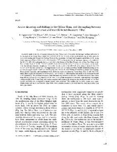
Figure 2 shows calculations of F11, ⫺F12兾F11, F22兾F11, F34兾F11, F33兾F11, and F44兾F11 at ␭ ⫽ 0.864 ␮m for a columnar PHM with reff ⫽ 40 ␮m and L兾2r ⫽ 2.5. The calculations were performed with the ray-tracing code developed by Hess et al.17 Phase function F11 shows the features that are typical of and well known for the pristine hexagon: The halo peaks at ⌰ ⫽ 22° and ⌰ ⫽ 46° (caused by two refractions, through a 60° and a 90° prism, respectively), a maximum at ⬃155° (one and two internal reflections), and the backscattering peak (external and internal reflections).8 The two halos consist of weakly polarized light (⫺F12兾F11 ⬇ 0 for ⌰ ⫽ 22° and ⌰ ⫽ 46°). The degree of linear polarization is at its maximum for ⌰ ⬇ 120° and becomes negative for ⌰ ⬎ 160°. For an extensive explanation of these features the reader is referred to Können.29 B. Fig. 1. The four ice-crystal models used in this research: PHM, IMP, IHM, and POLY. The size of a hexagonal crystal is given by its length L and so-called radius r. Depending on the magnitude of the aspect ratio 共L兾2r兲, the crystal is a column 共L兾2r ⬎ 1兲 or a plate 共L兾2r ⬍ 1兲.

For unpolarized incident light (e.g., direct sunlight), F11 and ⫺F21兾F11 represent the intensity and the degree of linear polarization, respectively, of the scattered light. Because they have primary influence on the POLDER and ATSR-2 measurements discussed below, F11 and ⫺F21兾F11 receive special attention in the following subsections. The F11 element is normalized as follows:

冕 冕 2␲

0

␲

F11(⌰)sin(⌰)d⌰d␸ ⫽ 4␲.

(2)

0

In what follows, scattering matrices are presented for the four ice-crystal models that were used for the evaluation of the POLDER and ATSR-2 measurements. The calculations were performed by use of the GO approximation, which holds when the crystal size is much greater than the wavelength of light. The basic characteristics of the four models are discussed in turn. A.

Pure Hexagonal Monocrystal

The PHM has a pristine hexagonal shape; i.e., the crystal consists of pure ice (no impurities or air bubbles) and has a perfectly smooth surface. The dimensions of the PHM are indicated by its length (L) and so-called radius (r) (Fig. 1). Depending on the magnitude of the aspect ratio 共L兾2r兲, the crystal is a column 共L兾2r ⬎ 1兲 or a plate 共L兾2r ⬍ 1兲. The effective radius reff of the crystal is defined here as the radius of a sphere that has the same volume as the hexagon:

冉

冊

9冑3 2 reff ⫽ rL 8␲ 4062

1兾3

.

APPLIED OPTICS 兾 Vol. 44, No. 19 兾 1 July 2005

(3)

Imperfect Hexagonal Monocrystal

The basic shape of the IMP is that of the PHM as described in Subsection 2.A. The imperfectness of the IMP refers to a certain degree of distortion of the surface of the hexagon. On the basis of the work of Macke et al.,30 Hess et al.17 obtained a representation of the imperfect hexagon by means of random changes in the normal vector nˆ of the model crystal’s surface every time a ray passed an air–ice interface. The change of nˆ is expressed in terms of a tilt zenith angle that varies randomly between 0 and a specific maximum value ␣. This parameter can be considered the degree of distortion of the crystal: The greater ␣, the more distorted the crystal surface. The effect of surface distortion on the phase function and degree of linear polarization is similar to the effect of explicitly treating surface roughness, which is described, e.g., by Yang and Liou.31 Figure 3 shows calculations of F11 and ⫺F12兾F11 at ␭ ⫽ 0.865 ␮m for ␣ ⫽ 0° (PHM) and ␣ ⫽ 10°, 20°, and 30° (IMP). The calculations were performed with the code of Hess et al.,17 which is an extended version of the code developed by Hess and Wiegner.16 The figure shows that, with increasing ␣, prominent features of the phase function, such as the 22° and 46° halos, the maximum at 155°, and the backscattering peak gradually disappear. For ␣ ⫽ 30° the phase function varies rather smoothly with scattering angle. This value is suitable for the representation of natural (irregular) ice crystals in clouds.17 Unless stated otherwise, IMPs will refer to imperfect hexagons with ␣ ⫽ 30° (the expression “moderately distorted,” used in Subsection 4.A below, refers to ␣ ⫽ 5°–7°). C.

Inhomogeneous Hexagonal Monocrystal

As for the IMP, the basic shape of the IHM is that of the PHM. The IHM was introduced by C.-Labonnote et al.21,22 and consists of a pure hexagon with spherical air-bubble inclusions. The GO approximation is used to calculate the course of rays within the hexagon but, when an air bubble is met, Mie theory is used to calculate the scattering by the inclusion. On the basis of a Monte Carlo approach the air bubbles are randomly distributed over the ice crystal at distances

Fig. 2. Scattering matrix elements for a columnar PHM with reff ⫽ 40 ␮m and L兾2r ⫽ 2.5 (L ⫽ 137.147 ␮m, r ⫽ 27.429 ␮m). The wavelength is 0.865 ␮m. Diffraction is included. The calculations were performed with the ray-tracing code developed by Hess et al.17 Indicated are the scattering angles related to the ATSR and POLDER measurements.

specified by a mean free path length ⬍ l ⬎ . The size of the air bubbles is characterized by a two-parameter ⌫ function with an effective radius reff and variance veff. C.-Labonnote et al.22 found that ⬍ l ⬎ ⫽ 10 ␮m, reff ⫽ 1.0 ␮m, and veff ⫽ 0.1 are suitable values for the representation of natural (inhomogeneous) ice crystals in clouds. These values were used for all IHM calculations presented in this paper.

Figure 4 shows calculations of the scatteringmatrix elements for a columnar IMP and IHM 共L兾2r ⫽ 2.5兲 and a platelike IMP and IHM 共L兾2r ⫽ 0.1兲, all with reff ⫽ 40 ␮m. Again, the wavelength is 0.865 ␮m. From consideration of phase function F11, it appears that the effects of adding air bubbles to the crystal and distorting the crystal’s surface are similar: F11 becomes rather featureless and shows only a 1 July 2005 兾 Vol. 44, No. 19 兾 APPLIED OPTICS

4063

(cf. Figs. 2 and 4). Like the phase function, the ⫺F12兾F11 element for the IMP reveals no halos. The strength and occurrence of halos in the ⫺F12兾F11 element for the IHM depend on the aspect ratio of the crystal: For the columnar IHM both halos are present, whereas for the platelike IHM only the secondary halo is present. For ⌰ ⬎ 50° the degree of linear polarization is generally positive and reaches its maximum somewhere from ⌰ ⫽ 80° to ⌰ ⫽ 120°. Beyond this scattering angle, ⫺F12兾F11 gradually decreases to 0, except for the platelike IHM, which reveals negative polarization for the backward scattering angles (except for ⌰ ⫽ 180°, where ⫺F12兾F11 is forced to 0). D.

Fig. 3. (a) Phase function 共F11兲 and (b) degree of linear polarization 共⫺F12兾F11兲 for a PHM and three types of IMP. The wavelength is 0.864 ␮m, and for all crystals reff ⫽ 40 ␮m and L兾2r ⫽ 2.5. The degree of surface distortion is indicated by the parameter ␣: the greater ␣, the more distorted the crystal surface of the IMP.

gradual variation with ⌰. For the IMP, the halos have completely disappeared, which is not surprising because the typical 60° and 90° angles of the hexagon are smoothed out by the introduction of the surface distortion. These angles are not affected by addition of air bubbles to the PHM, which explains why the phase function for the IHM still has a weak halo at ⌰ ⫽ 22°. Not only are the halos suppressed by distortion of the crystal surface or by addition of air bubbles to the ice crystal but also the forward peak for the IMP or the IHM is less pronounced than that of the PHM. In general, one can say that, by distorting the pristine hexagon or by making it inhomogeneous, one redistributes the energy that is present in the sharp features of the undisturbed phase function over larger scattering angles. Surface distortion and air bubbles have pronounced effects on the degree of linear polarization 4064

APPLIED OPTICS 兾 Vol. 44, No. 19 兾 1 July 2005

Disordered Polycrystal

The last crystal model that is described here is the POLY, which is approximated by a three-dimensional Koch fractal.24 This is a geometry that is obtained by the application of a growth model based on selfsimilar refinement of the crystal structure. The basis of the polycrystal is a regular tetrahedron. The first generation of the triadic Koch fractal is obtained if reduced tetrahedrons are placed on the triangular surfaces of the original tetrahedron. A higher-order generation is obtained if this procedure is repeated with a reduced tetrahedron of the preceding generation. For the calculations presented here a disorded version of the Koch fractal, obtained by addition of random displacements of the reduced tetrahedrons, was used. Figure 4 shows that F11 for the polycrystal and that for the other crystals are similar with respect to the absence of GO features. Nevertheless there are significant differences, both in the absolute sense (the POLY scatters more sideward than the other crystals) and, for example, in slope (dF11兾d⌰ over the 60°–180° interval is largest for the polycrystal). Of all the crystals considered here, the POLY has the weakest degree of linear polarization, whereas the strongest polarization is obtained with the two plates, for ⌰ from 80° to 90°. The degree of linear polarization of the two columns is in general between that of the POLY and the plates, except in the backward direction, where ⫺F12兾F11 of IHM0.1 deviates from that of the other crystals. 3. Quantities and Instruments for Evaluation

In this section, definitions of three quantities for the evaluation of the four ice-crystal models are given. These quantities are cloud reflectance (R), cloud spherical albedo (S), and cloud polarized reflectance 共Rp兲. The first two are both described in Subsection 3.A because the spherical albedo is directly related to the reflectance. Apart from giving definitions, we present model calculations of cloud reflectance to demonstrate the sensitivity of the cloud reflectance pattern to the shape of the ice crystal within the cloud. A first evaluation of the different ice crystal models is made by use of reflectance measurements made by ATSR-2.19 ATSR-2 is an imaging radiometer onboard

Fig. 4. Scattering matrix elements for IMPs, IHMs, and a POLY. The monocrystal is either a column 共L兾2r ⫽ 2.5兲 or a plate 共L兾2r ⫽ 0.1兲. reff ⫽ 40 ␮m for both IMPs and IHMs. The wavelength is 0.865 ␮m. Diffraction is included. The IMP, IHM, and POLY models are described by Hess et al.,17 C.-Labonnote et al.,21,22 and Macke,24 respectively.

the European Space Agency’s European Remote Sensing Satellite (ERS-2), which produces images of the Earth at three visible–near-infrared wavelengths (0.55, 0.66, and 0.865 ␮m) and four infrared wavelengths (1.6, 3.7, 10.8, and 11.9 ␮m). The instrument has been designed to observe the same scene in nadir view and forward view (view zenith angles 0°–25° and 52°–55°, respectively). One can use the dual-view

geometry to sample different parts of the phase function and thereby estimate the dominating crystal shape.32,33 In Subsection 4.A below, simulations of R at the nonabsorbing wavelength 0.865 ␮m for the two viewing geometries are compared with ATSR-2 measurements made over a tropical cirrus anvil. The spherical albedo and polarized reflectance are evaluated by use of the multiview capabilities of the 1 July 2005 兾 Vol. 44, No. 19 兾 APPLIED OPTICS

4065

POLDER instrument. POLDER is an imaging radiometer, with a wide field of view, that has provided the first global, systematic measurements of spectral, directional, and polarized characteristics of the solar radiation reflected by the Earth-atmosphere system. The first version of POLDER flew onboard the Japanese satellite ADEOS-1 and was operational from August 1996 until June 1997. To evaluate the various ice-crystal models we exploit both the directionality (Subsection 4.B below) and the polarization (Subsection 4.C) of POLDER, using measurements made of ice clouds observed at several parts of the globe. A.

Reflectance and Spherical Albedo

The cloud total reflectance (for short, reflectance) is defined as R(␮, ␮0, ␸ ⫺ ␸0) ⫽

␲I(␮, ␮0, ␸ ⫺ ␸0) , ␮0E

(4)

where I is the reflected radiance 关W m⫺2 nm⫺1 sr⫺1兴 and E is the solar irradiance 关W m⫺2 nm⫺1兴 at the top of the Earth’s atmosphere perpendicular to the solar beam. The Sun-view geometry is defined by ␮ ⫽ cos共␪兲 and ␮0 ⫽ cos共␪0兲, in which ␪ is the view zenith angle, ␪0 is the solar zenith angle, and ␸ ⫺ ␸0 is the relative azimuth angle. The complete distribution of R共␮, ␸ ⫺ ␸0兲 for fixed ␮0 is known as the bidirectional reflectance distribution function (BRDF). To illustrate that the cloud BRDF is sensitive to the assumed ice-crystal model, we show in Fig. 5 calculations of R for a PHM and an IMP, both with L兾2r ⫽ 2.5 and reff ⫽ 40 ␮m. The Sun is at ␪0 ⫽ 45°. The multiple-scattering part of the calculations was made with the Royal Netherlands Meteorological Institute doubling adding model (DAK).34,35 One of the striking features of the BRDF for the PHM cloud is a bright spot at ␪ ⫽ 45° and ␸ ⫺ ␸0 ⫽ 180°. As the Sun-view geometry corresponds to ⌰ ⫽ 180°, the high reflectance is caused by the strong backscattering peak of the PHM (Fig. 2, F11). The semicircular area of high reflectance corresponds to the local maximum of F11 at ⬃⌰ ⫽ 155° (caused by one and two reflections in the PHM). The area of lowest reflectance, for nadir viewing directions, coincides with the minimum of F11 共⌰⬃130°兲. For increasing ␪ and toward the antisolar horizon 共␸ ⫺ ␸0 → 0兲, the reflectance increases substantially. The corresponding scattering geometry is one of decreasing ⌰, leading to an increase in F11. Note that nadir darkening and limb brightening are caused not only by an increase in the phase function but also by multiplescattering effects. Because the variation of F11 with ⌰ is much less pronounced for the IMP than for the PHM, most of the distinct features in the BRDF have disappeared. What remains is a gradually varying pattern characterized by nadir darkening and brightening toward the antisolar horizon. The example of Fig. 5 demonstrates that the reflec4066

APPLIED OPTICS 兾 Vol. 44, No. 19 兾 1 July 2005

Fig. 5. Simulated BRDFs for an atmosphere containing (a) a PHM cloud and (b) an IMP cloud. The radial coordinate is viewing zenith angle ␪ (shown from 0° to 75°), and the azimuthal coordinate is viewing azimuth angle ␾, relative to the solar principal plane. The color scales represent the top-of-atmosphere reflectance. For both cases the cloud optical thickness is 10, the solar zenith angle is 45°, and the wavelength is 0.865 ␮m. The top-of-atmosphere albedos are 0.62 and 0.64 for the PHM cloud and the IHM cloud, respectively.

tance pattern is to a high degree determined by the choice of the cloud particle. Consequently, an observed pattern of cloud reflectance, e.g., by satellite, contains information on the shape of the cloud particle, which one can use to decide whether a certain ice-crystal model is suitable for simulating observed reflectances. The more viewing capabilities a satellite instrument has, the more thorough the evaluation of an ice-crystal model in terms of reflectances can be. The quantity that will be used for the analysis of POLDER reflectance measurements is cloud spherical albedo S, which follows from integration of the plane albedo, A共␮0兲, over all solar zenith angles [where the plane albedo is the integral of R共␮, ␮0, ␸

⫺ ␸0兲 over all viewing angles]:

冕 冕冕 冕 1

S⫽

A(␮0)␮0d␮0

0 1

⫽

0

2␲

0

1

R(␮, ␮0, ␸ ⫺ ␸0)␮␮0d␮d␸d␮0. (5)

0

In practice, it is not feasible to obtain values of S from satellite measurements, as each value would require a large set of reflectance measurements of the same ground segment covering the full range of viewing and solar angles. The spherical albedo, however, can be used to define a consistency test, which makes it possible to decide whether a certain ice-crystal model is adequate for simulation of the angular pattern of the cloud reflectance. On the basis of a measured value of the reflectance Rn共⌰n兲 obtained for viewing direction n 共n ⫽ 1, 2, . . . , Nd兲 and corresponding to scattering angle ⌰n, it is possible to retrieve the corresponding spherical albedo Sn共⌰n兲. Crucial steps in this retrieval are (a) the assumption of a certain ice-crystal model and (b) tuning of the plane-parallel cloud optical thickness to find agreement between modeled and measured reflectance. Once this tuning has been performed, the complete angular pattern of cloud reflectance is known and the cloud albedo can be calculated for each ␪0. To obtain Sn共⌰n兲, one repeats the procedure for all possible values of ␪0. The crux of the consistency test is that, if the correct ice-crystal model has been chosen, the spherical albedo is consistent for all scattering angles. Because the POLDER instrument views the same pixel under Nd viewing directions, it makes sense to define a mean spherical albedo S៮ for this pixel, where the averaging takes place over the POLDER viewing directions: S៮ ⫽

1 Nd

Nd

兺 Sn(⌰n). n⫽1

(6a)

For each viewing direction corresponding to a scattering angle ⌰, a spherical albedo difference ⌬S共⌰兲 can be defined (we drop the subscript n): ⌬S(⌰) ⫽ S៮ ⫺ S(⌰).

(6b)

This parameter can also be defined relative to the mean spherical albedo, which gives the relative spherical albedo difference ⌬Srel共⌰兲 for a certain pixel: ⌬Srel(⌰) ⫽

⌬S(⌰) . S៮

(6c)

By considering a large number of POLDER measurements for different Sun-view geometries, one can construct scatterplots of ⌬Srel as a function of ⌰. Al-

though the viewing capabilities of POLDER are limited, the scatterplots reveal significant coverage of the scattering-angle domain: 60° ⬍ ⌰ ⬍ 180°. In the ideal situation of a perfect match between the modeled angular pattern of the cloud reflectance and the POLDER measurements, ⌬Srel would be 0. In reality, however, one can expect ⌬Srel to be different from 0, in particular when there is disagreement between the real and the assumed ice-cloud particles. As was demonstrated above, the angular pattern of cloud reflectance is sensitive to the choice of ice-crystal model. Therefore it can be expected that the dependency of ⌬Srel on ⌰ will reveal information on which ice-crystal model is most suitable for describing light scattering in ice clouds. B.

Polarized Reflectance

Because polarized reflectances are sensitive to the shapes of cloud particles,36 the POLDER instrument offers a unique opportunity for considering the angledependent polarized reflected radiation fields of clouds for evaluation of ice-crystal models. The starting point is the polarized radiance defined by Ip ⫽ ␧(Q2 ⫹ U 2)1兾2,

(7)

where Q and U are the Stokes parameters that describe the state of linear polarization of the reflected radiation and ␧ ⫽ ⫾1. For reasons of convenience, Ip is normalized as follows, giving the polarized reflectance Rp (C.-Labonnote et al.22 refer to this quantity as normalized modified polarized radiance): Rp(␮, ␮0, ␸ ⫺ ␸0) ⫽

␮0 ⫹ ␮ ␲Ip(␮, ␮0, ␸ ⫺ ␸0) . (8) ␮0 E

Rp depends primarily on scattering angle ⌰, so comparisons of modeled and measured values of Rp as a function of ⌰ are expected to reveal independent information on the question of which ice-crystal model is most suitable for describing light scattering in ice clouds. The descriptions of the total and polarized reflectance given above and in this subsection, respectively, imply that measurements of both quantities can be used for testing ice-crystal models. The information on ice-crystal shape given by the total and the polarized reflectance is, however, not identical. In principle, all orders of scattering contribute to the total reflectance, whereas single scattering—which is the source of information on ice-crystal shape— primarily determines the polarized reflectance. Higher orders of scattering give small to vanishing degrees of polarization. This reasoning implies that, especially for optically thick clouds, the polarized reflectance contains a stronger signal of the ice-crystal shape than the total reflectance. In Section 4 we evaluate the four ice-crystal models described in Section 2, using first the total reflectance and then the polarized reflectance. 1 July 2005 兾 Vol. 44, No. 19 兾 APPLIED OPTICS

4067

Fig. 6. ATSR-2 measurements of the forward-to-nadir reflectance ratio 共Rforward兾Rnadir兲 as a function of Rnadir at 0.865 ␮m for a tropical anvil cloud situated over the Pacific Ocean (14 °N, 134 °E; 6 September 1996). Superimposed onto the measurements are simulations of the reflectance ratio by use of PHM2.5 and IMP2.5 for several degrees of distortion parameter ␣ (Subsection 2.B). With increasing Rnadir, the ice-cloud optical thickness increases according to the series 1, 2, 4, 8, . . . , 128. Simulations for ␣ ⬎ 20° and also for IHM0.1 and IHM2.5 closely resemble those for ␣ ⫽ 20° but are not shown.

4. Evaluation A.

ATSR-2 Reflectance

To perform a first test with pristine and distorted hexagonal ice crystals, we consider ATSR-2 measurements made over an area of gradually thinning anvil cloud streaming off the top of a deep convective cloud system in the tropical North Pacific.18 At the time of the overpass, the solar zenith angle was 23° and the nadir and forward viewing directions of ATSR-2 corresponded to scattering angles of 161° and 121°, respectively (indicated in Fig. 2). For the analysis presented in this section, both measurements and simulations of the 0.865 ␮m reflectance are plotted as the ratio of forward-to-nadir reflectance against nadir reflectance. The approach of using reflectance ratios was proposed in previous analyses of ATSR-2 observations of tropical cirrus.32,33 Baran et al.32 showed that, at nonabsorbing wavelengths such as 0.865 ␮m, the ratio between nadir and forward reflectances is not highly sensitive to either crystal size or aspect ratio but does contain information on crystal shape. Figure 6 shows the ATSR-2 forward-to-nadir reflectance ratio 共Rforward兾Rnadir兲 as a function of Rnadir for the anvil cloud described above. The figure reveals a substantial degree of scatter, which is most probably caused by imperfect colocation of the nadir and forward images or by the presence of different crystal types in the cloud.32 Superimposed onto the measurements are simulations of the reflectance ratio, assuming PHM2.5 and IMP2.5 for different degrees of distortion parameter ␣ (Subsection 2.B). With increasing Rnadir, the ice-cloud optical thickness (␶) in4068

APPLIED OPTICS 兾 Vol. 44, No. 19 兾 1 July 2005

creases according to the series 1, 2, 4, 8, . . . , 128. For Rnadir ⬍ 0.4 共␶ ⬍ ⬃8兲, ATSR-2 measurements are best simulated with ice clouds consisting of moderately distorted IMPs 共␣ ⫽ 5°–7°兲. Both the pristine PHM and the more strongly distorted IMP (␣ ⫽ 10° or ␣ ⫽ 20°) give inadequate representations of the measurements. Simulations for ␣ ⬎ 20° and also for IHM0.1 and IHM2.5 closely resemble those for ␣ ⫽ 20° but are not shown. Although the signal of crystal shape at high cloud optical thickness is weakened by multiple scattering, the tail of the distribution shown in Fig. 6 tends to suggest that the optically thickest clouds 共␶ ⬎ ⬃16兲 in this case are better simulated by use of a the pristine PHM than the distorted IMP. As remotely sensed crystal-shape information for optically thick clouds stems from the upper part of the cloud and that for optically thin clouds from layers deeper in the cloud, one may speculate that the simulations and measurements shown in Fig. 6 suggest that, for this particular case, the upper part of the cloud contains pristine crystals and that more irregular shapes are found deeper in the cloud. Although we emphasize that this is merely a speculation, it does not contradict other studies that indicate that, in certain cases, crystal shapes become more complex, and crystal edges become more rounded, from the top to the base of cirrus.37,38 Because the ATSR-2 measurements presented here represent only one specific case of tropical cirrus, and because ATSR-2 covers only a small range of scattering angles, the analysis given above does not provide enough information for a thorough evaluation of the various ice-crystal models. It is nevertheless encouraging that the forward-to-nadir reflectance ratio can be adequately simulated. In Subsection 4.B we use the multiview capability of the POLDER instrument to consider a moreextensive range of scattering angles. B.

POLDER-Derived Spherical Albedo

To construct scatter plots of ⌬Srel as a function of ⌰ for ice clouds we made a selection of global POLDER measurements. Only those measurements that satisfied the following conditions were selected: (i) surface type, ocean in the absence of sea ice; (ii) cloud cover, 100%; (iii) thermodynamic phase, ice; (iv) viewing direction, all except the Sun’s glitter; (v) number of viewing directions per pixel, ⱖ 7; (vi) minimum difference between minimum and maximum scattering angles per pixel, 50°. The thermodynamic phase was determined from the fact that dRp共⌰兲兾d⌰ for scattering angles in the rainbow area is different for water clouds and ice clouds.36,39,40 Since the conditions of 10 November 1996 were selected in previous studies22,27 and are considered to be representative, POLDER measurements made on that day were also used for the analysis presented here. The result of selection criteria (i)–(vi) is approximately 30,000 points (corresponding to as many scattering geometries) distributed over the globe but mainly in the mid-latitude areas. In contrast to the work of Chepfer et al.,26 which addresses the retrieval of ice-crystal

shapes by use of POLDER observations on a global scale, the present analysis is directed toward testing individual ice-crystal models for obtaining adequate simulations of global-scale measurements with a single ice-crystal model. The relative spherical-albedo difference ⌬Srel at 0.670 ␮m was calculated by use of the singlescattering models described in Section 2 and the discrete ordinates radiative transfer method developed by Stamnes et al.41 Figure 7 shows scatterplots of ⌬Srel as a function of scattering angle ⌰ for six icecrystal types: columnar PHM with aspect ratio 2.5 (labeled PHM2.5), polycrystal, platelike IMP and IHM with aspect ratio 0.1 (IMP0.1 and IHM0.1, respectively), and columnar IMP and IHM with aspect ratio 2.5 (IMP2.5 and IHM2.5, respectively). For all hexagonal crystals, reff ⫽ 40 ␮m. The standard deviation of the distribution of ⌬Srel for each crystal is listed in Table 1. The scatterplot for the pristine hexagon, PHM2.5, reveals a distinct wavelike pattern, which shows convincing similarity to the variation of singlescattering phase function F11 with scattering angle for 90° ⬍ ⌰ ⬍ 180° (cf. Fig. 3). Owing to the presence of this pattern, the standard deviation is relatively large (0.075). The pattern suggests that this icecrystal model does not adequately describe the radiative properties of the observed ice clouds. Better results are obtained if an irregular crystal (i.e., POLY, IMP, or IHM) is used to describe single scattering. For these crystals the wavelike pattern in ⌬Srel has disappeared, which is the result of the featureless variation of F11 with ⌰ (Figs. 3 and 4). Consequently, the standard deviations in ⌬Srel are smaller than those for PHM2.5 (Table 1). Although the POLY and IHM0.1 perform better than PHM2.5, the negative slope in F11 共dF11兾d⌰ ⬍ 0兲 causes the distribution of points in the scatter plot to be tilted. Most of the tilt is gone for hexagonal plate IMP0.1, but best results are obtained for the two hexagonal columns, IMP2.5 and IHM2.5. For these crystals the scatter in ⌬Srel is concentrated about 0 and the standard deviations are small: ⬃0.03, which is less than half of the values for the PHM and the POLY. In this respect it is worth mentioning that a previous analysis, based on aircraft measurements, initially revealed difficulties with the polycrystal.42 C. POLDER-Derived Polarized Reflectance

Figure 8 shows POLDER-derived values of polarized reflectance Rp at ␭ ⫽ 0.865 ␮m as a function of scattering angle ⌰ for measurements made all over the globe. The most frequently occurring measurements of Rp (density ⬎ 0.7) reveal that Rp ⬎ 0 over the entire range of scattering angle and that Rp has a weak maximum near ⌰ ⫽ 90°. Beyond this value Rp gradually decreases from an average of ⬃0.025 to 0 at ⌰ ⫽ 180°. In view of the considerable variation in ice-cloud optical thickness and geographical position, the consistent pattern of Rp as a function of ⌰ is remarkable and offers good prospects for simulating the measurements of polarized reflectance with one of the ice-crystal model candidates.

To attempt to simulate the dominant behavior of Rp共⌰兲 as revealed by the POLDER measurements, we derived a mean cloud optical thickness for all measurements of Rp shown in Fig. 8 and for each crystal type. The results are listed in Table 1. The simulations of Rp were performed for an average solar zenith angle of 35° and only for the solar principal plane, where polarization is strongest. The result of the calculations is shown by the black curves in Fig. 8. Although the curve for PHM2.5 coincides with most of the measurements for ⌰ ⬍ 110°, the derivative dRp兾d⌰ is not consistent with the general trend of measurements. For ⌰ ⬎ 110°, and particularly beyond 140°, model calculations and measurements strongly disagree, in terms of both absolute value and derivative.43 The conclusion here is consistent with the findings presented in the Subsection 4.B: The pristine hexagon does not adequately describe the radiative properties of the observed ice clouds. Again, better results are obtained for the irregular ice crystals (IMP, IHM, and POLY), although Fig. 8 suggests that some irregular crystals perform better than others. The polycrystal produces values of Rp that are systematically lower than most of the measurements, except in the backscatter region 共⌰ ⬎ 160°兲. Both the platelike IMP and the platelike IHM cause an overestimation of most of the polarization measurements for ⌰ ⬍ 130°. For larger scattering angles, IMP0.1 gives an adequate simulation of Rp but IHM0.1 tends to give too-low values, in particular for ⌰ → 180°. Rp is best simulated with an ice cloud consisting of columnar IMP or IHM crystals. The IHM performs better than the IMP for scattering angles up to ⬃110°. From 110° to 150° the reverse tends to be true. Both crystals give adequate simulations of Rp for the backscatter region. 5. Summary and Conclusions

The analysis presented here consists of an evaluation of four ice-crystal models designed for the simulation of the reflected radiation field of ice clouds. The four ice-crystal models are the pure hexagonal monocrystal (PHM), the imperfect hexagonal monocrystal (IMP), the inhomogeneous hexagonal monocrystal (IHM), and the disordered polycrystal (POLY). A first evaluation was performed by means of 0.865 ␮m dual-view reflectances measured by ATSR-2 over a tropical cirrus anvil of variable optical thickness. Adequate simulations of the forward-to-nadir reflectance ratio proved to be possible with model clouds consisting of moderately distorted IMPs (distortion parameter, ␣ ⫽ 5°–7°). The analysis tends to suggest that the optically thickest clouds 共␶ ⬎ ⬃16兲 in this case are better simulated by use of the pristine PHM. A more-detailed evaluation of the ice-crystal models was made by means of POLDER measurements of the bidirectional reflectance of ice clouds observed all over the globe. On the basis of an assumed ice-crystal model we used retrievals of ice-cloud optical thickness at 0.670 ␮m to calculate the equivalent cloud spherical albedo (S) for each POLDER pixel corresponding to a certain scattering angle. The multiview 1 July 2005 兾 Vol. 44, No. 19 兾 APPLIED OPTICS

4069

Fig. 7. Scatterplots of the relative spherical albedo difference [⌬Srel; Eqs. (6)] at ␭ ⫽ 0.670 ␮m as a function of scattering angle (⌰) for six ice-crystal models: columnar PHM 共L兾2r ⫽ 2.5兲; polycrystal, platelike IMPL兾2r, and IHML兾2r 共L兾2r ⫽ 0.1兲; columnar IMPL兾2r, and IHML兾2r 共L兾2r ⫽ 2.5兲. The standard deviations of the distributions for the different crystals are listed in Table 1. The color scale represents the density of the POLDER measurements normalized to the maximum density. The data set consists of 30,000 measurements of ice-cloud reflectance, made mainly in the midlatitude areas, on 10 November 1996.

4070

APPLIED OPTICS 兾 Vol. 44, No. 19 兾 1 July 2005

Table 1. Statistics Related to Figs. 7 and 8a

Ice-Crystal Model

Standard Deviation

Optical Thicknessb

IMP2.5 IMP0.1 IHM2.5 IHM0.1 PHM2.5 POLY

0.032 0.042 0.032 0.059 0.075 0.065

12.1 21.0 9.8 16.0 15.7 10.5

a

The first column lists the six ice-crystal types used for the calculations of the cloud spherical albedo (Fig. 7) and polarized reflectance (Fig. 8). The second column lists the standard deviations of the distributions of the relative spherical albedo differences shown in Fig. 7. The third column lists POLDER retrievals of ice-cloud optical thickness used to simulate polarized reflectances (black curves in Fig. 8). The values represent means of ⬃30,000 pixels distributed over the globe but mainly in the midlatitudes. b The frequency distributions of the optical thickness are highly positively skewed,22 with standard deviations of the order of the optical thickness itself.

capability of POLDER, which means that each pixel is viewed under different angles, allowed for the retrieval of the relative spherical albedo difference 共⌬Srel兲 on a pixel-by-pixel basis: ⌬Srel ⫽ 共S៮ ⫺ S兲兾S៮ , where S៮ is the average of S over the viewing angles of POLDER. Any dependency of ⌬Srel on scattering an-

Fig. 8. POLDER-derived values, displayed in colors, of the polarized reflectance [Rp; Eq. (8)] at ␭ ⫽ 0.865 ␮m as function of scattering angle ⌰. The color scale gives the density of the measurements normalized to the maximum density. The black curves represent model calculations of Rp for the same ice-crystal models as used for Fig. 7. The calculations were performed for mean cloud optical thicknesses as listed in Table 1, a solar zenith angle of 35°, and for the solar principal plane only. The POLDER measurements considered for this figure relate to the same cloudy pixels as used for the analysis of ⌬Srel.

gle ⌰ and departure from 0 is likely to point to differences between the single-scattering properties of the ice-crystal model and the particle that is actually present in the ice cloud. To identify these differences we constructed scatterplots of ⌬Srel as a function of ⌰ for the various ice-crystal models. The scatterplot for the PHM revealed distinct features that are directly related to the single-scattering phase function of the PHM, whereas the other, irregular, crystals give relatively uniform distributions of ⌬Srel close to 0. The distributions for the POLY and IHM0.1 (platelike inhomogeneous hexagon with aspect ratio 0.1) are tilted with respect to the ⌬Srel ⫽ 0 level, which is caused by a gradient in the single-scattering phase function. For the columnar or platelike IMP and for the columnar IHM the agreement between model calculations and measurements is nearly perfect, which indicates that with these crystals adequate simulation of the angular-dependent radiation field of the observed ice clouds at the wavelength considered is achieved. To exploit the sensitivity of the degree of polarization to cloud particle shape, we used polarized reflectance measurements made by POLDER to perform a final evaluation of the ice-crystal models. Again, the use of the pristine hexagon gives features in the reflected radiation field that are not present in the POLDER measurements. Better agreement between model calculations and measurements is obtained for the irregular ice crystals (IMP, IHM, and POLY), although the POLY produces polarized reflectances that are systematically lower than most of the measurements. The scattering-angle dependency of the polarized reflectance is best simulated with a model ice cloud consisting of columnar IMP or IHM crystals. Our overall conclusion in this paper is that adequate and best simulations of the total and polarized reflectance of the observed ice clouds at the wavelengths considered are obtained for model ice clouds consisting of hexagonal ice crystals with distorted surfaces (the IMP model) or hexagonal ice crystals containing air bubbles (the IHM model). Both models contain sufficient degrees of freedom in their structural parameters (aspect ratio, surface distortion, airbubble content) with which to obtain adequate simulations of the global-scale measurements considered. Both the evaluation in terms of the spherical albedo and polarized reflectance indicate that the pristine hexagon does not adequately describe the radiative properties of the observed ice clouds. In this context it should be mentioned that the size of the PHM used 共reff ⫽ 40 ␮m兲 plays an important role in the inadequacy of the simulations. The crystal is large enough for the geometrical optics approximation to be valid and to produce the typical features in the scattering phase function that are related to the geometrical shape of the crystal, which are in turn responsible for most of the deviations between model calculations and measurements. If small enough crystals are used, the GO approximation breaks down, so adequate simulations for pristine crystals may become possible. Note that for small crystals the 1 July 2005 兾 Vol. 44, No. 19 兾 APPLIED OPTICS

4071

approach presented here, which is based on raytracing techniques, cannot be followed. In this case the finite-difference time-domain method can be used.8,11 The possibility of using small ice crystals was previously addressed by Baran et al.,27 who also used spherical albedo comparisons based on POLDER measurements. Those authors used the method of improved geometrical optics44 to compute the single-scattering properties of a small randomly oriented hexagonal column. GO-based features may also be eliminated from the scattering-matrix elements by averaging the single-scattering properties of various particle shapes. An ensemble of shapes—such as a mixture of medium-sized hexagonal plates and columns, small quasi-spheres, and large irregular particles such as bullet rosettes22— has been observed or applied frequently.38,45–50 Although a mixture may be a good representation of the real situation in ice clouds, the strength of the IMP and IHM models lies in the relative simplicity of the models in combination with their demonstrated ability to simulate adequately the (polarized) reflected radiation field over ice clouds on a global scale. The research of W. H. Knap was financially supported by Space Research Organization Netherlands (project EO-025). We thank Andreas Macke (Institute for Marine Research, University of Kiel) for providing us with the single-scattering properties of the polycrystal. The comments of an anonymous reviewer are gratefully acknowledged. References and Notes 1. D. L. Hartmann, “Radiative effects of clouds on Earth’s climate,” in Aerosol–Cloud–Climate-Interactions, P. V. Hobbs, ed. (Academic, 1993), pp. 151–173. 2. T. F. Stocker, G. K. C. Clarke, H. Le Treut, R. S. Lindzen, V. P. Meleshko, R. K. Mugara, T. N. Palmer, R. T. Pierrehumbert, P. J. Sellers, K. E. Trenberth, and J. Willebrand, “Physical climate processes and feedbacks,” in Climate Change 2001: The Scientific Basis. Contribution of Working Group I to the Third Assessment Report of the Intergovernmental Panel on Climate Change, J. T. Houghton, Y. Ding, D. J. Griggs, M. Noguer, P. J. van der Linden, X. Dai, K. Maskell, and C. A. Johnson, eds. (Cambridge U. Press, 2001), pp. 417– 470. 3. M. I. Mishchenko, W. B. Rossow, A. Macke, and A. A. Lacis, “Sensitivity of cirrus cloud albedo, bidirectional reflectance and optical thickness retrieval accuracy to ice particle shape,” J. Geophys. Res. 101 (D12), 16973–16985 (1996). 4. M. Doutriaux-Boucher, J.-C. Buriez, G. Brogniez, L. C.-Labonnote, and A. J. Baran, “Sensitivity of retrieved POLDER directional cloud optical thickness to various ice particle models,” Geophys. Res. Lett. 27, 109 –112 (2000). 5. W. H. Knap, P. Stammes, and R. B. A. Koelemeijer, “Cloud thermodynamic phase determination from near-infrared spectra of reflected sunlight,” J. Atm. Sci. 59, 83–96 (2002). 6. Examples are hexagonal columns or plates, dendritic crystals, needles, and all sorts of complex-shaped crystals.7 Liou8 defines 11 ice-crystal habits that commonly occur in cirrus: solid and hollow columns, single and double plates and a plate with attachments, a bullet rosette with four branches, an aggregate composed of eight columns, a snowflake, a dendrite, and an ice particle with rough surfaces. 4072

APPLIED OPTICS 兾 Vol. 44, No. 19 兾 1 July 2005

7. A. H. Auer and D. L. Veal, “The dimensions of ice crystals in natural ice clouds,” J. Atmos. Sci. 27, 919 –926 (1970). 8. K. N. Liou, “Light scattering by atmospheric particulates,” in An Introduction to Atmospheric Radiation (Academic, 2002), pp. 169 –256. 9. F. M. Kahnert, “Numerical methods in electromagnetic scattering theory,” J. Quant. Spectrosc. Radiat. Transfer 79-80, 775– 824 (2003). 10. D. W. Mackowski, “Discrete moment method for calculation of the T matrix for nonspherical particles,” J. Opt. Soc. Am. A 19, 881– 893 (2002). 11. K. N. Liou, Y. Takano, and P. Yang, “Light scattering and radiative transfer in ice crystal clouds: Applications to climate research,” in Light Scattering by Nonspherical Particles, M. I. Mishchenko, J. W. Hovenier, and L. D. Travis, eds. (Academic, 2000), pp. 417– 449. 12. K. Sassen, N. C. Knight, Y. Takano, and A. J. Heymsfield, “Effects of ice-crystal structure on halo formation: cirrus cloud experimental and ray-tracing modeling studies,” Appl. Opt. 33, 4590 – 4601 (1994). 13. P. N. Francis, “Some aircraft observations of the scattering properties of ice crystals,” J. Atmos. Sci. 52, 1142–1154 (1995). 14. R. P. Lawson, A. J. Heymsfield, S. M. Aulenbach, and T. L. Jensen, “Shapes, sizes and light scattering properties of ice crystals in cirrus and a persistent contrail during SUCCESS,” Geophys. Res. Lett. 25, 1331–1334 (1998). 15. M. I. Mishchenko and A. Macke, “How big should hexagonal ice crystals be to produce halos?” Appl. Opt. 38, 1626 –1629 (1999). 16. M. Hess and M. Wiegner, “COP: a data library of optical properties of hexagonal ice crystals,” Appl. Opt. 33, 7740 –7746 (1994). 17. M. Hess, R. B. A. Koelemeijer, and P. Stammes, “Scattering matrices of imperfect hexagonal ice crystals,” J. Quant. Spectrosc. Radiat. Transfer 60, 301–308 (1998). 18. W. H. Knap, M. Hess, P. Stammes, R. B. A. Koelemeijer, and P. D. Watts, “Cirrus optical thickness and crystal size retrieval from ATSR-2 data using phase functions of imperfect hexagonal ice crystals,” J. Geophys. Res. 104 (D24), 31721–31730 (1999). 19. T. Edwards, R. Browning, J. Delderfield, D. J. Lee, K. A. Lidiard, R. S. Milborrow, P. H. McPherson, S. C. Peskett, G. M. Toplis, H. S. Taylor, I. Mason, G. Mason, A. Smith, and S. Stringer, “The Along Track Scanning Radiometer measurement of sea-surface temperature from ERS-1,” J. Briti. Interplanet. Soc. 43, 160 –180 (1990). 20. H. Woick, S. Dewitte, A. Feijt, A. Gratzki, A. P. Hechler, R. Hollmann, K.-G. Karlsson, V. Laine, P. Löwe, H. Nitsche, M. Werscheck, and G. Wollenweber, “The Satellite Application Facility on climate monitoring,” Adv. Space Res. 30, 2405– 2410 (2002). 21. L. C.-Labonnote, G. Brogniez, M. Doutriaux-Boucher, J.-C. Buriez, J.-F. Gayet, and H. Chepfer, “Modeling of light scattering in cirrus clouds with inhomogeneous hexagonal monocrystals. Comparison with in-situ and ADEOS–POLDER measurements,” Geophys. Res. Lett. 27, 113–116 (2000). 22. L. C.-Labonnote, G. Brogniez, J.-C. Buriez, M. DoutriauxBoucher, J.-F. Gayet, and A. Macke, “Polarized light scattering by inhomogeneous hexagonal monocrystals. Validation with ADEOS–POLDER measurements,” J. Geophys. Res. 106, 12139 –12153 (2001). 23. P.-Y. Deschamps, F.-M. Bréon, A. Podaire, A. Bricaud, J.-C. Buriez, and G. Sèze, “The POLDER mission: instrument characteristics and scientific objectives,” IEEE Trans. Geosci. Remote Sens. 32, 598 – 615 (1994). 24. A. Macke, “Scattering of light by polyhedral ice crystals,” Appl. Opt. 32, 2780 –2788 (1993).

25. W. B. Rossow and R. A. Schiffer, “ISCCP cloud data products,” Bull. Am. Meteorol. Soc. 71, 2–20 (1991). 26. H. Chepfer, P. Goloub, J. Riedi, J. F. De Haan, J. W. Hovenier, and P. H. Flamant, “Ice crystal shapes in cirrus clouds derived from POLDER兾ADEOS-1,” J. Geophys. Res. 106 (D8), 7955– 7966 (2001). 27. A. J. Baran, P. N. Francis, L. C.-Labonnote, and M. DoutriauxBoucher, “A scattering phase function for ice cloud: tests of applicability using aircraft and satellite multi-angle multiwavelength radiance measurements of cirrus,” Q. J. R. Meteorol. Soc. 127, 2395–2416 (2001). 28. H. C. van de Hulst, Light Scattering by Small Particles (Dover, 1981). 29. G. P. Können, Polarized Light in Nature (Cambridge U. Press, 1985). 30. A. Macke, J. Mueller, and E. Raschke, “Single scattering properties of atmospheric ice crystals,” J. Atmos. Sci. 53, 2813– 2825 (1996). 31. P. Yang and K. N. Liou, “Single-scattering properties of complex ice crystals in terrestrial atmosphere,” Contrib. Atmos. Phys. 71, 223–248 (1998). 32. A. J. Baran, P. D. Watts, and J. S. Foot, “Potential retrieval of dominating crystal habit and size using radiance data from a dual-view and multiwavelength instrument: a tropical cirrus anvil case,” J. Geophys. Res. 103 (D6), 6075– 6082 (1998). 33. A. J. Baran, P. D. Watts, and P. N. Francis, “Testing the coherence of cirrus microphysical and bulk properties retrieved from dual-viewing multispectral satellite radiance measurements,” J. Geophys. Res. 104 (D24), doi:10.1029兾 1999JD900842 (1999). 34. J. F. de Haan, P. Bosma, and J. W. Hovenier, “The adding method for multiple scattering calculations of polarized light,” Astron. Astrophys. 183, 371–391 (1987). 35. P. Stammes, “Spectral radiance modelling in the UV–visible range,” in IRS 2000: Current Problems in Atmospheric Radiation, W. L. Smith and Y. M. Timofeyev, eds. (Deepak, 2001), pp. 385–388. 36. H. Chepfer, G. Brogniez, and Y. Fouquart, “Cirrus clouds’ microphysical properties deduced from POLDER observations,” J. Quant. Spectrosc. Radiat. Transfer 60, 375–390 (1998). 37. A. J. Heymsfield and J. Iaquinta, “Cirrus crystal terminal velocities,” J. Atmos. Sci. 57, 916 –938 (2000). 38. A. J. Heymsfield and G. M. McFarquhar, “Midlatitude and tropical cirrus—microphysical properties,” in Cirrus, D. K. Lynch, K. Sassen, D. O’C. Starr, and G. Stephens, eds. (Oxford U. Press, 2002), pp. 78 –101. 39. P. Goloub, M. Herman, H. Chepfer, J. Riedi, G. Brogniez, P. Couvert, and G. Sèze, “Cloud thermodynamic phase classifi-

40.

41.

42.

43.

44.

45.

46. 47.

48.

49.

50.

cation from the POLDER spaceborne instrument,” J. Geophys. Res. 105, 14747–14759 (2000). J. Riedi, M. Doutriaux-Boucher, and P. Goloub, “Global distribution of cloud top phase from POLDER兾ADEOS-I,” Geophys. Res. Lett. 27, 1707–1710 (2000). K. Stamnes, S.-C. Tsay, W. Wiscombe, and K. Jayaweera, “Numerically stable algorithm for discrete-ordinate-method radiative transfer in multiple scattering and emitting layered media,” Appl. Opt. 27, 2502–2509 (1988). P. N. Francis, J. S. Foot, and A. J. Baran, “Aircraft measurements of the solar and infrared radiative properties of cirrus and their dependence on ice crystal shape,” J. Geophys. Res. 104 (D24), 31685–31696 (1999). The peak in the measurements of Rp at ⌰ ⬇ 140° may be related to the presence of a small fraction of water clouds in the selected data. P. Yang and K. N. Liou, “Geometric-optics-integral-equation method for light scattering by non-spherical ice crystals,” Appl. Opt. 35, 6568 – 6584. G. M. McFarquhar and A. J. Heymsfield, “Microphysical characteristics of three cirrus anvils sampled during the Central Equatorial Pacific Experiment (CEPEX),” J. Atmos. Sci. 53, 2401–2423 (1996). H. R. Pruppacher and J. D. Klett, Microphysics of Clouds and Precipitation, 2nd ed. (Kluwer Academic, 1997). G. M. McFarquhar, A. J. Heymsfield, A. Macke, J. Iaquinta, and S. M. Aulenbach, “Use of observed ice crystal sizes and shapes to calculate mean-scattering properties and multispectral radiances: CEPEX April 4, 1993, case study,” J. Geophys. Res. 104 (D24), 31763–31780 (1999). P. Rolland, K. N. Liou, M. D. King, S. C. Tsay, and G. M. McFarquhar, “Remote sensing of optical and microphysical properties of cirrus clouds using Moderate-Resolution Imaging Spectrometer (MODIS) channels: methodology and sensitivity to physical assumptions,” J. Geophys. Res. 105 (D9), 11721– 11738 (2000). P. Yang, B. Gao, B. A. Baum, W. J. Wiscombe, Y. X. Hu, S. L. Nasiri, P. F. Soulen, A. J. Heymsfield, G. M. McFarquhar, and L. M. Miloshevich, “Sensitivity of cirrus bidirectional reflectance to vertical inhomogeneity of ice crystal habits and size distributions for two Moderate-Resolution Imaging Spectroradiometer (MODIS) bands,” J. Geophys. Res. 106 (D15), 17267– 17292 (2001). J. R. Key, P. Yang, B. A. Baum, and S. L. Nasiri, “Parameterization of shortwave ice cloud optical properties for various particle habits,” J. Geophys. Res. 107 (D13), doi:10.1029兾 2001JD000742 (2002).

1 July 2005 兾 Vol. 44, No. 19 兾 APPLIED OPTICS

4073