Modeling Transportation Networks and Urban Traffic ...

Modeling Transportation Networks and Urban Traffic Dynamics: A Markovian Framework by

Xilei Zhao

A thesis submitted to The Johns Hopkins University in conformity with the requirements for the degree of Master of Science.

Baltimore, Maryland May, 2017

c Xilei Zhao 2017

All rights reserved

Abstract

An urban transportation network is a complex and stochastic system with high degrees of unpredictability and uncertainty. While significant advances have been in modeling dynamic network traffic, existing efforts usually involve high cost in data acquisition and overly complex methods for modeling the physics of traffic. In this thesis, we propose a novel approach for modeling dynamic network traffic using the Markovian framework and the integrated route and link data. Such data are readily available from Google Maps. In particular, by applying maximum likelihood (ML), we propose a statistical method to capture the complexities of transportation networks by integrating data from the full systems (origin-destination (O-D) travel times) and subsystems (traffic condition for links). After using ML to estimate links’ travel times and obtaining the turning probabilities at intersections, we put forward a Markov chain model to simulate the dynamic network traffic with a transition matrix determined from real-world data. Finally, we present a case study in downtown Baltimore to illustrate the approach and validate the model. This Master’s thesis is based on a journal paper submitted to Transportation ii

ABSTRACT

Research Part C: Emerging Technologies with James C. Spall.

Reader: James C. Spall

iii

Acknowledgments I would like to thank my advisor, James C. Spall for helping me accomplish this challenging task. His wisdom enlightens me, his enthusiasm inspires me, and his kindness elevates me. He has taught me how to become a rigorous and independent researcher. He is a great mentor and close friend to me. I am so blessed to have him as my advisor, and I look forward to collaborating with him further in the future. I also would like to thank my Ph.D. advisor Judith Mitrani-Reiser for her unwavering support for my work and future career. I especially appreciate her patience, intelligence, and kindness. I would like to thank my colleagues, Karla Hernandez, Long Wang, Jingyi Zhu, among many others, for their generous help in my research. Thanks to the Department of Applied Mathematics and Statistics and the Department of Civil Engineering for their support of my multidisciplinary research interests. I also want to thank my friends here at Hopkins, who have never left me during ups and downs throughout these years: Sen Lin, Xiaohui Tu, Zhiye Li, Qian Ke, Zhixuan Yang, Luoluo Liu, Xinyi Lin, Zhaohao Fu, Qi Wang, Yang Yang, Ian Miers, Gwen Chodur, Sriram Sankaranarayanan, Jimi Oke, Gary Lin, Mikhail Osanov, and

iv

ACKNOWLEDGMENTS

many others. I especially want to thank my dear friends back in China, who have loved me, missed me, and cheered me up when I felt down: Xin Pan, Cheng Chen, and Lili Wang. I would like to express my deepest gratitude to my family members. I am extremely grateful to my parents, Xiaolin Shen and Guoquan Zhao, for raising me and loving me unconditionally. They have worked very hard to nurture me and provide me all the resources I needed for a better education. I would like to thank my late grandpas, Tiehan Shen and Rongzu Zhao, for their deep love and great support for my choices since I was a little girl. I also want to thank my other family members, especially my aunts, uncles, cousins, and grandmas, for bearing my bad temper and loving me anyway. Finally, I would like to thank Xiang (Jacob) Yan for being my boyfriend and “editor-in-chief ” for my writings. Since four years ago when we first met each other, he has always been nothing but supportive, inspirational, and encouraging. He completes me: his wit and patience show me the way of being a better researcher, while his love and empathy make me become a better human-being.

v

Dedication This thesis is dedicated to my younger cousins, Zehui Yin and Xiyang Shen.

vi

Contents

Abstract

ii

Acknowledgments

iv

List of Tables

x

List of Figures

xi

1 Introduction

1

1.1

Motivation . . . . . . . . . . . . . . . . . . . . . . . . . . . . . . . . .

1

1.2

Markovian framework . . . . . . . . . . . . . . . . . . . . . . . . . . .

3

1.3

Summary of thesis contents . . . . . . . . . . . . . . . . . . . . . . .

6

2 Methodology

7

2.1

Markov chain formulation . . . . . . . . . . . . . . . . . . . . . . . .

9

2.2

Maximum likelihood formulation and parameter estimation . . . . . .

11

2.2.1

Basic definitions and properties of maximum likelihood estimation 11

vii

CONTENTS

2.3

2.2.2

Maximum likelihood function for transportation network . . .

12

2.2.3

Relationship between full systems and subsystems . . . . . . .

16

2.2.4

Uncertainty bounds and the Fisher information matrix formulation . . . . . . . . . . . . . . . . . . . . . . . . . . . . . . .

19

Estimation of transition matrix . . . . . . . . . . . . . . . . . . . . .

21

3 Case Study 3.1

3.2

26

Network and model estimation . . . . . . . . . . . . . . . . . . . . . .

26

3.1.1

Data collection strategy . . . . . . . . . . . . . . . . . . . . .

27

3.1.2

MLE results . . . . . . . . . . . . . . . . . . . . . . . . . . . .

32

Applications . . . . . . . . . . . . . . . . . . . . . . . . . . . . . . . .

33

3.2.1

Uncertainty bounds for MLEs . . . . . . . . . . . . . . . . . .

33

3.2.2

Markovian simulation . . . . . . . . . . . . . . . . . . . . . . .

34

4 Conclusions and Future Work

37

4.1

Major contributions . . . . . . . . . . . . . . . . . . . . . . . . . . . .

37

4.2

Limitations . . . . . . . . . . . . . . . . . . . . . . . . . . . . . . . .

39

4.3

Future work . . . . . . . . . . . . . . . . . . . . . . . . . . . . . . . .

39

A Identifiability Proof

41

B Derivation of Sample Correlation Coefficient’s Distribution for Bivariate Bernoulli Case

44

viii

CONTENTS

C Estimation Results for Network in Downtown Baltimore

46

Bibliography

48

Vita

54

ix

List of Tables 3.1

MLEs and 95% confidence intervals for routes within the network . .

34

C.1 Sample means and MLEs for links’ success probabilities . . . . . . . .

47

x

List of Figures 1.1

Markovian framework for modeling dynamic network traffic . . . . . .

2.1

A general transportation network: solid lines denote network of interest (A-B-C-D-E-F-G-H-I-J); dashed lines denote boundary layer. . . . . . Illustration of transition matrix: submatrix P for links within the network and remaining elements in P 0 for incoming and outgoing traffic streams. . . . . . . . . . . . . . . . . . . . . . . . . . . . . . . . . . .

2.2

3.1

3.2 3.3

A transportation network in downtown Baltimore (approximately 1 mile east of the center of the Inner Harbor area): solid lines denote network of interest (A-B-C-D-E-F-G-H-I-J-K-L-M-N-O-P); dashed lines denote boundary layer. . . . . . . . . . . . . . . . . . . . . . . . . . . Link data collection strategy: data for links in subset 1 are collected on different days than links in subset 2. . . . . . . . . . . . . . . . . . Histogram of travel time (origin: link 70; destination: link 54) . . . .

xi

4 8

11

27 29 35

Chapter 1 Introduction

1.1

Motivation

Congestion, accidents, greenhouse gas emissions, noise, and pollution are the five principal issues with high traffic densities for large-scale urban networks [Schlote, 2014]. Congestion, especially, has brought tremendous harm to our society, both economically and environmentally. According to a report by the U.S. Federal Highway Administration (FHWA) [Federal Highway Administration, 2016], “while the congestion problems faced by travelers and freight shippers in the metropolitan regions of more than one million people consume more travel time and waste more fuel than congestion faced in cities less than 500,000, the burden and frustration has increased across all population groups.” If urban planners and transportation engineers can have a firm grasp on the dynamics of urban network traffic and better predict po-

1

CHAPTER 1. INTRODUCTION

tential congested areas, they might come up with preventative measures to deal with traffic congestion. Therefore, it is essential to develop reliable methods to model the dynamic network traffic, especially during rush hours. Ideally, these models should be easily implementable across regions at a fairly low cost in order to ensure widespread usage. This thesis proposes a novel Markov model for dynamic network traffic using integrated route and link data that are readily available from Google Maps. We show how state-of-the-art methods in system identification can be used to estimate the unknown parameters in the model through a combination of data on links and on selected routes in the network of interest. Modeling dynamic network traffic has been an ongoing theme in the field of transportation engineering for decades. One major effort is to model dynamic traffic assignment using analytical or simulation-based methods [Ziliaskopoulos, 2001]. Analytical approaches mainly include mathematical programming (e.g., [Merchant and Nemhauser, 1978, Daganzo, 1994, Daganzo, 1995]), optimal control (e.g., [Ran et al., 1993,Lo et al., 2001,Di Gangi et al., 2016]), and variational inequality (e.g., [Nagurney, 2013]). On the other hand, simulation-based methods have gained wide popularity in the research area of modeling dynamic traffic assignment, such as [Peeta and Mahmassani, 1995, Ben-Akiva et al., 2012, Papathanasopoulou et al., 2016]. In recent years, some researchers (e.g., [Crisostomi et al., 2011,Moosavi and Hovestadt, 2013,Schlote, 2014]) started to use Markov chains to model traffic dynamics, which has proved to be simple and effective. The Markovian work in modeling dynamic network traffic

2

CHAPTER 1. INTRODUCTION

has multiple useful applications, especially in the areas of transportation planning and engineering (e.g., [Crisostomi et al., 2011, Moosavi and Hovestadt, 2013]), and sustainable transportation infrastructure (e.g., [Schlote, 2014]). While significant results exist in the modeling of dynamic network traffic, existing efforts usually suffer from high cost in data acquisition, impractical assumptions in simulation, or overly complex methods for modeling the physics of traffic.

1.2

Markovian framework

Building on previous work, we propose to address the issues above by developing a novel Markovian framework (as shown in Figure 1.1) for modeling urban traffic dynamics. The approach relies on recently developed statistical methods in ML [Spall, 2014,Zhao and Spall, 2016] to capture the complexity of traffic networks. Open-source data for the method are conveniently available from Google Maps. Specifically, we extend the existing Markov model [Crisostomi et al., 2011] by estimating the most probable travel time for each traffic link using integrated route and link data, and includes the incoming and outgoing traffic streams to the network of interest. As shown in Figure 1.1, the Markov model relies on unknown parameters to estimate travel times for links and turning probabilities for intersections. In this study, we only address the part related to travel time estimation for links by using integrated route and link data from Google Maps, without exploring better estimation methods

3

CHAPTER 1. INTRODUCTION

for turning probabilities. To estimate the parameters for travel times for links, we first model a transportation network as multi-level systems. Within the network, we identify the traffic condition on a link as a subsystem, while the O-D travel time for a specific route as a full system. We compute maximum likelihood estimates (MLEs) for the mean output for the success rates for links and travel times for routes based on data from full systems and subsystems.

Figure 1.1: Markovian framework for modeling dynamic network traffic

A major reason for using the MLE-based full-system/subsystem technique is that complicated connections exist between the full system traffic behavior (routes’ travel times) and the subsystem traffic flow (links’ success rates). That is, the complexities 4

CHAPTER 1. INTRODUCTION

of network traffic (e.g., traffic incidents, work zones, bad weather, poor traffic signal timing, etc.) cannot be readily modeled mathematically, but the MLEs based on test data can make full use of information at both link levels and O-D levels to properly represent these connections and implicitly capture the physics of traffic. The full-system/subsystem technique as applied to a single route has been proved simple and easy-to-implement [Zhao and Spall, 2016]; this thesis extends the idea to full networks. Further, we derive the Fisher information matrix (FIM) and use it to compute confidence intervals for major routes’ travel time estimates. To implement the MLE-based idea above, we need data to populate the model for traffic networks. Ideally, any data source that can output traffic condition on links and travel time for routes is suitable for this study. In the field of transportation engineering, real data usually come from sensors, cameras, and probe vehicles; however, these traditional data sources have their own limitations, such as being hard to acquire, expensive to purchase, limited in quantity, biased in data sampling (such as using taxi data to represent all travelers’ behavior), etc. The real-time traffic data available on Google Maps overcomes these limitations. Most importantly, Google Maps is an open-source platform with real-time traffic condition information and O-D travel time estimates provided by its users within the network. As an opensource platform, data acquisition and high cost problems of traditional data sources are solved by using Google Maps. Furthermore, instead of hiring drivers to collect probe data or using taxi GPS data, Google Maps has a large quantity of users. The

5

CHAPTER 1. INTRODUCTION

users include common car drivers, Uber/Lyft drivers, truck drivers, and others, who provide free GPS data to Google Maps in real time, helping to solve the problems of limited data points and biased data. Compared to the traditional data sources, Google Maps has another advantage: it provides traffic data over small, medium, or large towns or municipalities throughout the country, providing the data needed to implement the Markov approach here. Moreover, in terms of data quality, some previous studies (e.g., [Ozimek and Miles, 2011, Wang and Xu, 2011]) have verified the applicability and accuracy of Google Maps data.

1.3

Summary of thesis contents

The remainder of the thesis is organized as follows: in Chapter 2, we introduce the mathematical modeling process, including three major steps, i.e., Markov chain formulation, ML formulation and parameter estimation, and transition matrix estimation. In Chapter 3, we give a numerical example in downtown Baltimore, in which we also propose a link data collection strategy and provide empirical evidence to show independence of test data by following this strategy. Finally, we conclude the thesis by discussing the strengths and limitations of the approach, and then suggest areas for future study.

6

Chapter 2 Methodology First, we introduce the basic definitions about the traffic network. As shown in Figure 2.1, taking a small general transportation network as an example, we first define the boundary of network, and in this example, the boundary is Square ACIG. All the traffic links within Square ACIG are considered for analysis. Note that the different directions of a link are considered as two distinct links. For example, in Figure 2.1, link AB, from west to east, and link BA, from east to west, are treated as two separate links. Specifically, as shown in Figure 2.1, links within the network are shown in orange, incoming traffic streams are denoted as green arrows, and outgoing traffic streams are identified as red arrows. The links and nodes in the dashed border (“boundary layer”) will play a role in modeling entry and exit to the network of interest, shown in solid lines. The reminder of the Chapter is divided into three parts. In Section 2.1, we briefly

7

CHAPTER 2. METHODOLOGY

introduce the Markov chain formulation. In Section 2.2, we discuss how to model a transportation network as full systems (routes) and subsystems (links), and derive the MLEs and associated Fisher information to facilitate the estimation of transition matrix. Then, in Section 2.3, we show how the transition matrix is fully identified for modeling dynamic network traffic.

Figure 2.1: A general transportation network: solid lines denote network of interest (A-B-C-D-E-F-G-H-I-J); dashed lines denote boundary layer.

8

CHAPTER 2. METHODOLOGY

2.1

Markov chain formulation

In this section, we will briefly introduce the basic definitions and properties of Markov chain, in order to facilitate the derivation of transition matrix estimation in Sections 2.2 and 2.3. A discrete time Markov chain presents a random process that transits from one state to another state on a state space. First, let us recall some basic definitions about Markov chains. Consider a stochastic process with discrete state via discrete time Y 0 , Y 1 , Y 2 , .... The sequence is a Markov process if the following relationship holds for all τ = 0, 1, 2, ...:

P Y τ+1 |Y 0 , Y 1 , ..., Y τ = P Y τ+1 |Y τ Therefore, the probability of moving to the next state at time step τ + 1 depends only on the present state at time step τ and not on the previous state. That is, using a Markovian model, we can predict the future state of the process solely based on its current state without knowing the full history of the process. We let state Y τ = [yτ1 , yτ2 , ..., yτp ]T be a vector that denotes the location of a given vehicle among the p links of time τ (hence, Y τ is a unit vector with a 1 in one location and with 0s in all others). For example, as illustrated in Figure 2.1, if link AB corresponds to link 1, then yτ1 is a binary component of state Y τ , which represents whether a vehicle is traveling on link AB, in the direction from node A to node B. At state Y τ , if the vehicle is traveling on link AB, then yτ1 is equal to 1 with 9

CHAPTER 2. METHODOLOGY other elements equal to 0, i.e., Y τ = [1, 0, 0, ..., 0]T . While the Markov assumption is unrealistic from a driver’s perspective, because a driver’s behavior is based on the known origin and destination and his or her movement within the network is largely predetermined, we, as external observers, do not know what the driver’s intention is in the next moment, and thus his or her movement in the network seems random from our perspective, which makes Markov assumption reasonable to capture the stochastic nature of dynamic traffic network. The Markov process within a transportation network with p links can be completely described by a p-by-p transition matrix P . For example, if the chain is currently in state Y τ (corresponding to one arrangement: yτa = 1, a ∈ {1, 2, ..., p} and other elements = 0), then it moves to state Y τ+1 (another arrangement: yτ+1,b = 1, b ∈ {1, 2, ..., p} and other elements = 0) with transition probability pab . Note that pab is one of the entries of P . The core of our Markovian framework is the transition matrix estimation. Figure 2.2 shows the overall transition matrix P 0 we need to estimate, including a submatrix P for links within the network, and other elements in P 0 to represent incoming and outgoing traffic streams. We first focus on how to estimate P , which requires travel time estimation for links and turning probability estimation for intersections. In the next section, we show a full-system/subsystem technique to estimate links’ success probabilities using ML formulation with integrated link and route data from Google Maps, which will be applied to compute links’ travel time in Section 2.3.

10

CHAPTER 2. METHODOLOGY

Figure 2.2: Illustration of transition matrix: submatrix P for links within the network and remaining elements in P 0 for incoming and outgoing traffic streams.

2.2

Maximum likelihood formulation and parameter estimation

2.2.1

Basic definitions and properties of maximum likelihood estimation

The ML formulation involves a parameter vector θ to be estimated and a loglikelihood function log L(θ) to be maximized. The method of ML is a powerful tool for estimating parameters and is perhaps the most popular general method in practice [Scholz, 2006], relative to other statistical methods such as method of moments. Next, let us introduce some basic concepts and definitions of MLE. According to the 11

CHAPTER 2. METHODOLOGY

definition of MLE (for example, see [Rice, 2006, pp. 267–268]), suppose that random variables X1 , ..., Xn have a joint density or frequency function p(x1 , x2 , ..., xn |θ). Given observed values Xi = xi , where i = 1,..., n, the likelihood of θ as a function of x1 , x2 , ..., xn is defined as L(θ) = p(x1 , x2 , ..., xn |θ). The likelihood function is a function of θ, given all the observed data. The MLE of θ maximizes the likelihood function by fully utilizing the observed data. If we have independent, identically distributed (i.i.d.) data, we can easily write down the log-likelihood function as:

log L(θ) = log

n Y

p(xi |θ) =

i=1

2.2.2

n X

log p(xi |θ).

i=1

Maximum likelihood function for transportation network

Consider a transportation network system that consists of p links. We define the traffic conditions on links as subsystems, so we have p subsystems in this case. The links are modeled as binary subsystems with “0” (“failure”) for congested links and “1” (“success”) for non-congested links. We assume that test data for all the links, including within and across the links, are independent. Data are collected on different event days to help ensure independence. The test data for link j, where j = 1, 2, · · · , p, are i.i.d., because we suggest collecting one data point for link j at a 12

CHAPTER 2. METHODOLOGY

specific time on one day; that is to say, for link j, test data collected on day 1 is i.i.d. from test data collected on day 2. We do not assume data across links are identically distributed; that is, the success probability generally varies by link. For data across links at a given time and day, distant links can be viewed as nearly independent, whereas the traffic conditions of adjacent links may influence each other. Therefore, we propose a novel link data collection strategy in Subsection 3.1.1 to resolve the data problem of potential dependence. A full system is defined as the travel time from origin to destination through a specific route. Obviously, it is hard to include all the links in one route, so we need to collect data for several full systems in order to cover all the traffic links within the network. We assume that test data for all the full systems are independent. Even though full system data might have some statistical dependence across different routes, we try to minimize the dependence by properly choosing full systems. Note that formal experimental design for full system data collection [Spall, 2003, Chap. 17] might be used here for collecting data efficiently and optimally, but we do not consider that in this thesis. It is also worth pointing out that full system data and subsystem data are not collected on the same day in order to ensure independence. We assume the full system outputs (the O-D travel times along a specific route) follow the log-normal distribution. The log-normal assumption for travel times has been applied in many previous studies (for example, [El Faouzi and Maurin, 2007,Zhao and Spall, 2016]). The logic behind it is simple and straightforward: a log-normal

13

CHAPTER 2. METHODOLOGY

distribution is defined on positive real numbers, which well fits the nature of travel time; a log-normal distribution is skewed to the right, with right tail representing traffic delay. In [Zhao and Spall, 2016], we tested the distribution of travel time data collected from Google Maps against the log-normal assumption, and a large P -value was obtained (well above the common thresholds of 0.05 or 0.01), indicating that travel time data are consistent with a log-normal distribution. Let us now define θ and describe our notation for the data.

We use semi-

colon to represent a separate row for convenience (e.g., [a, b; c, d] denotes a 2 × 2 matrix with rows a, b and c, d). Suppose that data are collected for r full sys  tems in the network. Let ζ = ω1 , σ21 ; ω2 , σ22 ; ...; ωr , σ2r represent an r-by-2 matrix with ωi and σ2i representing unknown means and variances of the normally distributed logarithm of the outputs of the r full systems. Let ρj represent the success probabilities for subsystem j, j = 1, 2, ..., p. The parameter vector θ ≡  T ρ1 , ρ2 , ρ3 , ..., ρp ; elements in ζ are not included in the parameter vector to be estimated because they are uniquely determined by θ and relevant constraints. Let T = 

T11 , T12 , ..., T1,k(1) ; T21 , T22 , ..., T2,k(2) ; ...; Tr1 , Tr2 , ..., Tr,k(r)



indicate the collection of

observed, scalar-valued full system output Tqi from k(q) i.i.d. experiments on the full system q, q = 1, 2, ..., r, representing the O-D travel times through route q in the traffic network. Because we assume the full system outputs follow log-normal distri bution as described above, we let Z = Z11 , Z12 , ..., Z1,k(1) ; Z21 , Z22 , ..., Z2,k(2) ; ...; Zr1 , Zr2 , ..., Zr,k(r)



=



log(T11 ), log(T12 ), ..., log(T1,k(1) ); log(T21 ), log(T22 ), ..., log(T2,k(2) );

14

CHAPTER 2. METHODOLOGY ...; log(Tr1 ), log(Tr2 ), ..., log(Tr,k(r) ) represent the normally distributed collection of log-transformed full system outputs, which can facilitate the following derivation. We now derive the log-likelihood function based on the full set of data: subsystem (link) and full system (O-D pairs). According to the definition of log-normal distribution and the properties of independent experiments, the log-likelihood function for full system outputs is r X  q=1

k(q)  1 X k(q) 2 log(σq ) − 2 − (Zqj − ωq )2 + constant, 2 2σq j=1

(2.1)

where the full system parameters (i.e., ωq , σq , q = 1, 2, ..., r) can be fully represented by θ (which will be discussed later). Let Xji represent the ith output of the jth subsystem, indicating traffic conditions (failure “0” or success “1”) on the link j. Thus, the number of successes in n(j) i.i.d. experiments on subsystem j, j = 1, 2, ..., p, can be expressed as Sj ≡

n(j) X

Xji .

i=1

Because the Xji follow a Bernoulli distribution, the log-likelihood function of subsystem outputs is p X   Sj log(ρj ) + (n(j) − Sj ) log(1 − ρj ) .

(2.2)

j=1

By adding (2.1) and (2.2), the log-likelihood function for the entire system, including

15

CHAPTER 2. METHODOLOGY

all the full system test data and the subsystem test data, is:

log L(θ) =

r X  q=1

k(q)  k(q) 1 X 2 − log(σq ) − 2 (Zqj − ωq )2 2 2σq j=1 p X   + Sj log(ρj ) + (n(j) − Sj ) log(1 − ρj ) + constant. (2.3) j=1

In order to maximize eqn.(2.3), we differentiate the log-likelihood function to obtain the score vector: ∂ log L(θ) = ∂θ

r X



− k(q) h0q2 (θ) + 2σ2q q=1

k(q) h0q2 (θ) X (Zqj 2σ4q j=1

− ωq )2 +

k(q) h0q1 (θ) X (Zqj σ2q j=1

    +   

 − ωq ) 

 S1 ρ1

−

n1 −S1 1−ρ1

.. . Sp ρp

−

np −Sp 1−ρp

    , (2.4)   

where h0q1 (θ) and h0q2 (θ) represent the gradients of hq1 (θ) and hq2 (θ) with respect to θ, for q = 1, 2, ..., r. The vector [hq1 (θ), hq2 (θ)]T relates θ to [ωq , σ2q ], reflecting the relationship between full system q and the ρ subsystems. Next, we will show how to derive hq1 (θ) and hq2 (θ).

2.2.3

Relationship between full systems and subsystems

Following the precedent in [Zhao and Spall, 2016], the typical travel time of each link under different traffic conditions (“0” or “1”) is computed as follows according 16

CHAPTER 2. METHODOLOGY

to the color scheme for Google Maps:     lj /v if the link is blue or yellow (“1”),    lj /v 0

(2.5)

if the link is red or dark red (“0”),

where v and v 0 are the mean travel speeds in different traffic conditions estimated from historical Google Maps data (different from data T and Z) and lj represents the length of the link j. We treat v and v 0 as fixed parameters, not estimates, in the ¯ j = Sj /n(j) represent the observed success rate on link j using analysis below. Let X only link data, for j = 1, 2, ..., p. Based on (2.5), we derive the typical travel time on each link and its expectation as follows: ¯j × tj = X

lj ¯ j ) × lj , + (1 − X v v0

lj lj lj v − v0 E(tj ) = ρj × + (1 − ρj ) × 0 = 0 − lj ρj v v v vv 0

(2.6)

where tj represents the typical travel time of link j, j = 1, 2, ..., p. Then, as shown in [Zhao and Spall, 2016], we are able to derive the relationship between full systems and subsystems, relating θ to ζ. Specifically, for full system q, suppose there are m(q) links within this specific route (full system), and the corresponding parameters of the links in full system q can be represented as a sub-sequence of θ with m(q) components. Obviously, m(q) ≤ p (the number of links within the network). For example, suppose full system 1 contains link 1, 3, and 6; then, m(1) = 3, ρ11 = ρ1 , ρ12 = ρ3 , and ρ13 = ρ6 .

17

CHAPTER 2. METHODOLOGY

To derive the relationship between full systems and subsystems, we use two equivalent ways (one from the full system perspective, the other from the subsystem perspective) to represent the expectation and variance for the ith observation of the qth full system. We then equate these results to obtain hq1 and hq2 . Based on the log-normal assumption for the full system output, we can write down the expectation and variance for Tqi using the log-normal properties [Johnson et al., 1994]: 1 E(Tqi ) = exp (ωq + σ2q ), 2

(2.7)

Var(Tqi ) = [exp (σ2q ) − 1] exp (2ωq + σ2q ).

(2.8)

We then derive the expectation and variance for Tqi by using the subsystem information [Zhao and Spall, 2016]: m(q)

E(Tqi ) =

X  lqj j=1

v0

−

 v − v0 lqj ρqj 0 vv

(2.9)

m(q)

Var(Tqi ) =

X  v − v0  2 ) (1 − ρ ) ρ l ( q q q j j j vv 0 j=1

(2.10)

where lqj represents the length of the link qj . The expectation and variance derived from the full systems are required to be equal to those derived from the subsystems. That is, eqn.(2.7) and eqn.(2.9) are equivalent and eqn.(2.8) and eqn.(2.10) are equivalent. Therefore, we have developed the relationship between full systems and subsystems. The implicit function theorem (e.g., see [Apostol, 1974, pp. 373–374]) provides conditions under which there is a vector [hq1 (θ), hq2 (θ)]T , relating θ to [ωq , σ2q ], where q = 1, 2, ..., r. Thus, let 18

CHAPTER 2. METHODOLOGY ˆ indicate the MLE of ωq , and σ ˆ indicate the MLE of σ2 (we are ˆ q = hq1 (θ) ˆ 2q = hq2 (θ) ω q using the invariance property of MLE: a function of an MLE is also an MLE). Let M =   Pm(q)  Pm(q)  0 0 0 0 0 2 l /v − (v − v )/(vv ) · l ρ ; V = ((v − v )/(vv ) · l ) ρ (1 − ρ ) . q q q q q q j j j j j j j=1 j=1 Then, we obtain hq1 (θ) and hq2 (θ) as   1 V +1 , hq1 (θ) = log M − log 2 M2   V +1 . hq2 (θ) = log M2 After obtaining hq1 (θ) and hq2 (θ), we are able to compute h0q1 (θ) and h0q2 (θ) in the score vector, eqn.(2.4). Solving the score equation, ∂ log L(θ)/∂θ = 0, yields a candidate MLE for θ and reflects a careful balancing of information between the full system and subsystems. In general, the solution to the score equation is not unique and can only be achieved numerically.

2.2.4

Uncertainty bounds and the Fisher information matrix formulation

Aside from providing an MLE of θ (and derived parameters ωi , σ2i ), we are also able to produce uncertainty bounds (confidence regions) on the estimates. The confidence regions are based on asymptotic normality of the estimator with a covariance matrix derived from the FIM for θ [Spall, 2014]. The FIM contains a summary of the amount of information in the data with respect to the quantities of interest (see [Spall, 2003, Sect. 13.3]). The FIM has multiple applications, including confidence region 19

CHAPTER 2. METHODOLOGY

construction, model selection, experimental design, etc. In this thesis, our interest ˆ i, σ ˆ 2i . centers on the use of FIM for constructing confidence regions for the estimates, ω The FIM for θ is defined as ∂log L(θ) ∂log L(θ) F N (θ) = E · ∂θ ∂θT

!

! log ∂ 2 L(θ) = −E . ∂θ∂θT

In this thesis, the p × p FIM FN (θ) for a twice-differentiable log-likelihood function, log L(θ), is given by

F N (θ) =

r  X q=1

 k(q) 0 k(q) 0 0 T 0 T h (θ)hq2 (θ) + h (θ)hq1 (θ) + J N (θ), (2.11) 2(hq2 (θ))2 q2 hq2 (θ) q1

  where J N (θ) = diag n(1)/(ρ1 (1 − ρ1 )), · · · , n(p)/(ρp (1 − ρp )) . One of the most significant properties of the MLE and FIM is asymptotic normality. In this thesis, we are only considering uncertainty in ωq . Based on asymptotic distribution theory described in Spall (2014), we have ˆ q ∼ N (ωq , h0q1 (θ)T F N (θ)−1 h0q1 (θ)), ω

(2.12)

for full system q where q = 1, 2, · · · , r and sufficiently large sample sizes. In practice, ˆ on the right hand side of (2.12). Expression (2.12) can be we often set θ equal to θ ˆ q , and can also be adapted used to compute the asymptotic uncertainty bounds for ω to give uncertainty bounds on travel time reliability for any O-D pairs in the network (even those for which full system data were not collected).

20

CHAPTER 2. METHODOLOGY

2.3

Estimation of transition matrix

In order to estimate the transition matrix, we take three key factors into account: network topology (connectivity of links), turning probabilities, and time homogeneity of the network. These three key factors fully determine the entries of transition matrix. We now show how the ML formulation in Section 2.2 can be elegantly combined with the assumptions of a Markov chain in order to estimate the unknown entries in the transition matrix. As illustrated in Figure 2.1, at time step r, it is obvious that if a vehicle is in link BE with yj = 1 for link j corresponding to link BE, the vehicle may stay in link BE or turn to neighboring link EF, EH, or ED at time step τ + 1. Let us consider the turning case first. Considering the network topology or links connectivity, link BE only connects to these three links, with zero probability to turn to other traffic links within the network. Besides, the probabilities of moving from link BE to these three links may be different, depending on the turning probabilities at intersection E. Next, let us discuss the alternative possibility: before the vehicle reaches intersection E, the vehicle will have non-zero probability of staying on link BE at time step τ + 1 (with no knowledge of where the vehicle’s exact location on the link), which depends on a lot of factors, such as traffic condition on the link, travel speed, length of link, and time unit of the Markov chain. Among all these factors, choosing a proper time unit from one state to the next state is very significant for the Markovian framework. Note that if the time unit is large, the transition matrix will have all di21

CHAPTER 2. METHODOLOGY

agonal elements very close to zero. On the contrary, if the time unit is very small, the transition matrix will nearly be an identity matrix, since the vehicle is almost certain to stay on the current link. However, a large time unit may violate the Markovian nature of the chain, whereas a small time unit makes the problem trivial and cannot help us model the road traffic dynamics. Hence, an appropriate time unit, ∆t, needs to be determined for analysis. Ref. [Moosavi and Hovestadt, 2013] points out that by choosing a proper time unit, the resulting Markovian model captures important factors like traffic flow, speed, and traffic lights, which were neglected in traditional network analysis. The choice of ∆t is highly related to the travel time estimates for each link within the network. According to eqn.(2.6) and the MLE estimates for θ obtained in Section 2.2, we are able to obtain the MLE estimates for tj : v − v0 lj lj ρˆj , tˆj = 0 − v vv 0

(2.13)

where ρˆj represents the MLE estimates of success probability for link j, j = 1, 2, ..., p. In order to make sure all the diagonal elements of P are non-negative, the time unit ∆t must satisfy ∆t ≤ min(tˆ1 , tˆ2 , ..., tˆp ). Next, after determining the MLEs of the traffic links and the time unit ∆t, it is natural to compute sj ≡ tˆj /∆t, where sj represents the number of steps needed before the vehicle reaches the intersection at the end of the link. Then, the corresponding

22

CHAPTER 2. METHODOLOGY

estimate for the probability of the vehicle staying on the current link is pˆjj =

sj − 1 , sj

(2.14)

where pˆjj represents the diagonal element for row j in P . Next, we need to estimate the off-diagonal entries of the transition matrix (i.e., scaled turning probabilities). A link is at most connected to three neighboring links for a lattice-type network, so there are at most three off-diagonal entries in a row. Hence, for large p, the transition matrix is a sparse matrix. In this thesis, we assume that estimates of turning probabilities are available for all the intersections in the network. The estimates can be obtained by collecting relevant data through sensors, cameras, or probe vehicles, and then using various estimation approaches, such as [Maher, 1984,Mirchandani and Head, 2001,Chen et al., 2012]. The estimated turning probabilities need to be scaled to serve as the off-diagonal entries of the transition matrix in order to ensure the sum of row equal to 1 (see eqn.(2.16)). Another important issue is how to model the incoming and outgoing traffic flows as relates to the entries in P 0 that are not in P . Clearly, vehicles are not trapped in the network, so we need to allow vehicles to enter and leave the network of interest freely. To resolve this issue, we add the entrances and exits of the network into the analysis, as illustrated in the boundary layer of green arrows and red arrows in Figure 2.1. Specifically, as shown in Figure 2.2, we expand the transition matrix from p × p to (p + q) × (p + q), where q is the number of incoming and outgoing links of the network. In Figure 2.1, we have p = 24 and q = 24; so the ultimate transition 23

CHAPTER 2. METHODOLOGY

matrix that considers incoming and outgoing flows is 48 × 48. For each entrance to the network, denoted by green arrows in Figure 2.1, the diagonal entry equals to 0 and the off-diagonal entries are purely determined by the network connectivity and turning probabilities. Other states of the Markov chain can never transfer to these entrances. For exits to the network, denoted by red arrows in Figure 2.1, the diagonal entry equals to 1; in other words, the Markov chain will be absorbed in these exits. Intuitively, the entrances of the network can allow vehicles entering the network at time step 0 of the Markov chain and these vehicles will transfer to other neighboring links immediately at time step 1; the exits of the network allow vehicles leaving the network forever as the vehicles reach these absorbing states. Note that, in this thesis, we do not consider the special situation where a vehicle leaves the network and then comes back in a short time period. To sum up, the full transition matrix P 0 can be determined. In particular, the diagonal entries are estimated by    sj −1   for links within the network  sj     0 pˆjj = 0 for entering links         1 for exiting links,

24

(2.15)

CHAPTER 2. METHODOLOGY

and the off-diagonal entries can be obtained as      (1 − pˆ0jj ) × fˆji for links within the network      0 pˆji = fˆji for entering link j         0 for exiting link j,

(2.16)

where fˆji is the estimated turning probability from link j to link i for i 6= j and i, j = 1, 2, · · · , p + q. Without assuming the stationary distribution exists for the Markov chain (which is the major assumption of previous work [Crisostomi et al., 2011,Moosavi and Hovestadt, 2013,Schlote, 2014]), we are able to identify all the parameters of the transition matrix. Identifiability is an important property that a statistical model needs to satisfy in order to draw formal conclusions and make concrete predictions. The model is identifiable if it is theoretically possible to compute the true values of the model’s parameters, when the sample size goes to infinity. Our model is locally identifiable, with full proof provided in Appendix A. Previous work (e.g., [Crisostomi et al., 2011,Moosavi and Hovestadt, 2013,Schlote, 2014]) and our thesis all assume that the Markov chain is time-homogeneous. Clearly, travel times and turning probabilities are time-dependent [Skabardonis et al., 2003, Van Lint and Van Zuylen, 2005]. In practice, several different transition matrices will be needed to capture differences in traffic flow throughout the day, and each of those matrices will need to be periodically updated to capture long-term (e.g., seasonal) changes in traffic dynamics or network topology. 25

Chapter 3 Case Study

3.1

Network and model estimation

Let us now give a case study for downtown Baltimore to illustrate the overall framework. The transportation network is selected as shown in Figure 3.1, where there are 72 links in total with 46 links within the network and 13 entering links and 13 exiting links in the boundary layer. Note that the street between node I and node E and the street between node E and node A are one-way streets. So only two links (i.e., link IE and link EA) are considered for these two streets.

26

CHAPTER 3. CASE STUDY

Figure 3.1: A transportation network in downtown Baltimore (approximately 1 mile east of the center of the Inner Harbor area): solid lines denote network of interest (A-B-C-D-E-F-G-H-I-J-K-L-M-N-O-P); dashed lines denote boundary layer.

3.1.1

Data collection strategy

For the full systems, we collect travel time data for different routes in the network (Google Maps allows for a choice of specific routes and then provides real-time travel time estimates based on the route choices). In this case study, we consider 12 full systems/routes in collecting data for this network (M-N-O-P-L-H-D; M-I-E-A-B-C-D; D-H-L-P-O-N-M; D-C-B-A; M-I-J-K-L-H; I-E-F-G-H-D; M-N-J-F-B-C; C-B-F-J-NM; N-O-K-G-C-D; D-C-G-K-O-M; D-H-G-F-E; H-L-K-J-I-M). These 12 full systems were chosen because the 12 routes cover all 46 traffic links within the network and 27

CHAPTER 3. CASE STUDY

because the 12 routes have few overlaps of links in order to minimize correlation among full systems. Formal experimental design for how to choose full systems to collect data might be beneficial for this study, but we do not consider such design here. For the subsystems, we collect real-time “color” data, representing live traffic conditions in four categories. That is, we use the Google Maps color scheme: green = normal traffic conditions, yellow = slower traffic conditions, red = congestion, and dark red = nearly stopped or stop-and-go traffic shown on links by choosing the “traffic” option in the menu of Google Maps. A green or yellow is a “1” (success) while a red or dark red is a “0” (failure). When collecting the link data, we need to minimize the correlation among those links. Therefore, we propose the following link data collection strategy: by splitting the links within the network into two subsets (see Figure 3.2), we collect one data point for either subset 1 or subset 2 on one day, which guarantees data for subset 1 are independent of data for subset 2. Moreover, within a subset, there is no adjacent links considered; for instance, as shown in Figure 3.2(a), link JK (considered in subset 1) is directly connected to link KG, KL, and KO, none of which are considered in subset 1. In this case, the link data collection strategy reduces the dependence of data between the two subsets; also, within a subset, links are not directly connected to each other, helping to reduce dependence.

28

CHAPTER 3. CASE STUDY

(a) Subset 1

(b) Subset 2

Figure 3.2: Link data collection strategy: data for links in subset 1 are collected on different days than links in subset 2.

29

CHAPTER 3. CASE STUDY

In this study, we collected 16 observations for each full system and 11 – 27 observations for each subsystem from Google Maps for this network at 5pm on certain weekdays (from Monday to Friday except for U.S. legal holidays) from March 31, 2016 through December 16, 2016. In order to evaluate the performance of the data collection strategy, we provide the following empirical evidence. Here, we use hypothesis testing to test whether the link data are independent. To be specific, we use Barnard’s exact test [Barnard, 1947] to test the null hypothesis that any link pairs within subset (subset 1 or 2) are independent versus the alternative that any link pairs within subset (subset 1 or 2) are not independent. We compute the appropriate test statistic and P -values for all link pairs within subsets, and there are 15 out of 415 (around 4%) that are below the 0.05 threshold. The 0.05 threshold indicates if the data are independent, we should expect 5% of the test statistics to have P -values lower than 0.05. In this case, we have 4% (quite close to 5%) of the P -values lower than 0.05 threshold, which is consistent with the assumption of the independence of test data. In addition to the overall assessment above, and in order to reduce the multiple comparison problem, we use the Bonferroni correction [Bonferroni, 1936] to test each individual hypothesis at 0.05/415 = 0.00012. The smallest P -value obtained above is 0.0053 (much larger than 0.00012), so the Bonferroni correction cannot reject the null hypothesis. That is, by following the above data collection strategy, evidence is consistent with the hypothesis that link data are independent.

30

CHAPTER 3. CASE STUDY

In order to check the results of independence test, we also test whether the correlation coefficients between links are equal to zero. In other words, we test the null hypothesis that the correlation coefficient ρ for any link pairs within a subset (subset 1 or 2) is equal to 0 versus the alternative that the correlation coefficient ρ for any link pairs within a subset (subset 1 or 2) is not equal to 0. We first derive the sample correlation coefficient’s distribution for the bivariate Bernoulli case (details are shown in Appendix B). Under the null hypothesis, we have ρ = 0 and γ2 = 1 in the asymptotic distribution for the sample correlation coefficient r computed from the observed binary link data (see eqn.(B.2)). According to (B.1) and γ2 = 1, we have r converges to normal distribution with mean zero and variance 1/N , when sample size N is large. That is,   1 . r → 0, N

(3.1)

Based on (3.1), we compute the P -values for all link pairs within subsets. We find that 26 out of 415 (around 6%) are below 0.05 threshold. Similarly, the 0.05 threshold indicates if the data are uncorrelated (i.e. ρ = 0), we should expect 5% of the sample correlation observations to have P -values lower than 0.05. In this case, we have 6% (quite close to 5%) of the P -values lower than 0.05 threshold, which supports the null hypothesis that the link data are uncorrelated. Therefore, the correlation test results are consistent with our independence test results, which overall gives us a stronger evidence that by following the data collection strategy, the link data are independent.

31

CHAPTER 3. CASE STUDY

3.1.2

MLE results

Using the data collection strategy in Subsection 3.1.1 and MLE method in Section 2.2, the estimates for subsystem success probabilities are shown in Appendix C. In contrast to the indicated sample means from only link data, it is expected that the MLEs for the links better represent the true success probabilities since the MLEs implicitly incorporate link interactions via the full system data. Taking link 46 as an example, the sample mean for subsystem link data alone is 1.00, but after incorporating full system information, the MLE for the success probability in link 46 decreases to 0.80. As one application of the above, we are able to identify vulnerable links (low subsystem success probabilities) within this network. For instance, in this network, link 2 has relatively low success probability, 0.54, compared to other links within the network. We may also notice that the success probability of link 2 is substantially lower than the links connected to it, namely, link 1, link 3, link 29, and link 38. Traffic engineers might wish to look into link 2 to figure out the reason behind this issue and try to address it in order to improve mobility. Besides, by using the baseline model and disaster management knowledge, the transition matrix may be properly modified for modeling adverse situations that occur on links, such as flooding, blast, and fire, in order to inform decision making and emergency planning. After properly modeling the transportation network and obtaining the success probabilities on links as discussed above, we are able to compute sj and thus pˆjj in 32

CHAPTER 3. CASE STUDY

eqn.(2.14). Then, if the turning probabilities at 5pm on a weekday are available for this network, i.e., fˆij is known, we will be able to obtain the transition matrix for this transportation network, according to eqn.(2.15) and (2.16).

3.2 3.2.1

Applications Uncertainty bounds for MLEs

After obtaining the MLEs for the transportation network, we are able to use (2.12) to compute the uncertainty bounds for any routes within the network (including full systems and other routes with no data collected). As an illustration of the results that can be obtained, Table 3.1 shows the MLEs and their corresponding 95% confidence intervals for four routes: the first three are full systems, and the last one is a new route with no data collected. According to the MLEs for θ as shown in Appendix C, we are able to compute MLEs for the full system parameter matrix ζ. For Route 1, we have hq1 = −2.7581, ˆ 1 ), when which corresponds to the MLE for the mean of Route 1 travel time (i.e., ω measured in units of log (hour). For the short travel time less than 1 hour, the value of hq1 is less than zero. We can transform the MLE of ω1 back to original travel time domain, which is 60eωˆ 1 = 3.80 min. By using (2.12), we are able to compute the ˆ 1 . Based on the asymptotic normality in (2.12), the 95% uncertainty bounds for ω ˆ 1 is [3.71, 3.90] min. Uncertainty bounds for full system travel confidence bound for ω 33

CHAPTER 3. CASE STUDY

time estimates are very useful for various stakeholders. For example, the uncertainty bounds show the estimation uncertainty of the MLEs, which can be used in planning in order to be sufficiently conservative with respect to potential public sector investments or in terms of deciding any other strategy that may affect the public. In particular, it would not be good to make a decision based on an overly optimistic estimate, and the uncertainty bounds give the decision-making a formal basis for being rationally conservative. Table 3.1: MLEs and 95% confidence intervals for routes within the network Number

Route

MLE (min)

95% confidence interval (min)

1

M-N-O-P-L-H-D

3.80

[3.71, 3.90]

2

M-I-E-A-B-C-D

3.85

[3.74, 3.96]

3

M-I-J-K-L-H

3.50

[3.37, 3.64]

4

H-L-K-J-I

2.44

[2.36, 2.53]

3.2.2

Markovian simulation

Based on the network model obtained in Section 3.1, we are able to estimate the transition matrix, simulate the Markov chain, and compute the typical travel time for a random O-D pair regardless of routes (in Subsection 3.2.1, we show MLEs and confidence intervals for random O-D pairs with specified routes).

34

CHAPTER 3. CASE STUDY

To be specific, in the application in Baltimore here, we first compute the links’ travel time estimates according to eqn.(2.13), and choose the time unit ∆t as 20s, which satisfies ∆t ≤ min(tˆ1 , tˆ2 , ..., tˆ46 ) as discussed in the previous Chapter. Then, we are able to compute the diagonal elements of the Markov chain based on eqn.(2.15). Here, we assume equal turning probabilities for each intersection, since we did not collect turning probability data from the actual network (e.g., in case where a left turn, right turn, or straight option is allowed, each probability is 1/3). In this case, the off-diagonal elements of the Markov chain are also obtained by using eqn.(2.16).

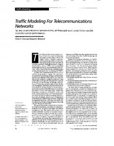
Figure 3.3: Histogram of travel time (origin: link 70; destination: link 54)

Next, we simulate the Markov chain and calculate the typical travel time from

35

CHAPTER 3. CASE STUDY

link 70 to link 54 regardless of route choices. Specifically, we take link 70 as the entrance and link 54 as the exit, meaning that we simulate vehicles that start at link 70 and ends at link 54. We then run Monte Carlo simulation 4,000 times and only save the traces of the 97 vehicles that end at link 54. Because there are 12 exits in this network and vehicles can leave at any exits during the simulation; we only care about the vehicles that leave at link 54. Figure 3.3 shows a histogram of the travel time for those vehicles exiting at link 54. The travel time for a random O-D pair has an overall log-normal-type shape (although not necessarily a formal log-normal distribution since the histogram represents an amalgamation of several route choices). The mode, median, and mean of the empirical distribution of travel time for these 97 vehicles are equal to 4.33 min, 4.33 min, and 4.85 min, respectively. Google Maps also provides a travel time estimate of “typically 4 min” for this O-D pair if the vehicle leaves at 5pm on a weekday. Finally, even though we assume equal turning probabilities for this network, the typical travel time obtained by simulations is consistent with Google Maps.

36

Chapter 4 Conclusions and Future Work

4.1

Major contributions

This thesis introduces a novel method to model dynamic network traffic using Markov chain and integrated route and link data. A Markovian framework is developed to model dynamic network traffic by using the most probable links’ travel time and considering incoming and outgoing traffic streams to the network of interest, which makes the traffic dynamics model much more realistic and applicable. Specifically, we use the MLE formulation and real-time data from Google Maps to estimate the most probable travel time of each link within the network, by extending the previous effort in applying the full-system/subsystem technique to a single route [Zhao and Spall, 2016] to a general transportation network. Notably, we also show the full identifiability of all the parameters without using the stationary distri-

37

CHAPTER 4. CONCLUSIONS AND FUTURE WORK

bution of Markov chain that lots of previous related work (such as [Crisostomi et al., 2011,Moosavi and Hovestadt, 2013]) in Markov modeling requires. In the case study, we put forward a new data collection strategy for traffic links, and provide empirical evidence to show the independence of data by following this strategy. Furthermore, we apply the FIM to compute the asymptotic uncertainty bounds for the travel time of major routes within the network. We also propose a novel method to compute the typical travel time for any random O-D pairs within the network using Monte Carlo simulation (and reflecting that multiple routes are associated with a given O-D pair). This work has the potential to be applied in the field of transportation planning and engineering, and many other areas such as traffic control [Crisostomi et al., 2011,Spall and Chin, 1997], community detection [Moosavi and Hovestadt, 2013], and pollution chain and electric vehicle chain modeling [Schlote, 2014]. One major contribution of the work is that the proposed network model based on applying the full-system/subsystem technique and integrated route and link data from Google Maps can provide a good estimate for links’ travel time. The method implicitly takes into account the complexities of traffic dynamics due to its reliance on full route data. Also, Google Maps, as an open data source, has proved to be user-friendly and effective. In addition, compared to previous Markov models, the Markovian framework proposed here is more realistic and applicable by using formal estimates for links’ travel times, relaxing the assumption of stationarity for the state probabilities, and considering incoming and outgoing traffic flows. The approach

38

CHAPTER 4. CONCLUSIONS AND FUTURE WORK

shown here provides a potential tool to decision makers that goes beyond capability in Google Maps by providing rigorous uncertainty bounds for travel time estimates, and helping urban planners and transportation engineers discover vulnerable links, understand traffic dynamics, and come up with better strategies to boost mobility. Moreover, the estimated transition matrix could also be modified to consider emergent scenarios on links (e.g., flooding, blast, fire, etc.) in order to facilitate emergency planning and enhance community resilience.

4.2

Limitations

The main limitations of the work are that turning probabilities need to be obtained as an important input to the Markovian framework; the full system/route data collected within one day might not be fully independent as discussed in the Chapters 2 and 3; and the full system data collection (i.e., which routes to choose and how many data to collect in each route) might not be optimal. All of the above can, in principle, be addressed with additional resources.

4.3

Future work

In future work, we hope to come up with an optimal full system data collection strategy using statistical experimental design. Furthermore, we plan to model the transportation performance under hazards (e.g., flooding, fire, blast, etc.) by prop39

CHAPTER 4. CONCLUSIONS AND FUTURE WORK

erly modifying the baseline Markov model, and then conducting global sensitivity analysis to identify vulnerable traffic links during emergent scenarios. Such efforts could demonstrate broad potential for application of the methodology to the fields of traffic management, emergency management, urban planning, community resilience, sustainability, and smart cities.

40

Appendix A Identifiability Proof The formal definition of identifiability is [Rothenberg, 1971]:

Definition 1: A parameter point a0 in the domain is said to be identifiable if there is no other parameter points in the domain which is observationally equivalent (i.e., implying the same probability distribution for the observable random variable).

However, global identifiability may be hard to achieve, so we introduce the concept of local identifiability [Rothenberg, 1971], which will be used later in the proof.

Definition 2: A parameter point a0 is said to be locally identifiable if there exits an open neighborhood of a0 containing no other parameter points in the domain which is observationally equivalent.

41

APPENDIX A. IDENTIFIABILITY PROOF

Next, we introduce the conditions that are necessary for the identifiability proof.

Condition 1: Google Maps’ data are collected independently for full systems (route travel times) and subsystems (links’ traffic condition): 1) on one day, collect either full system data or subsystem data; 2) if collecting full system data, one data point is collected for each full system on one day (assume full system data are independent); 3) if collecting subsystem data, one data point is collected for each subsystem within subset 1 or 2 (see Subsection 3.1.1) on one day (assume subsystem data are independent).

Condition 2: Subsystems all have positive number of samples, i.e., n(j) ≥ 1 for all j.

Condition 3: The turning probabilities at intersections that are within and/or on the boundary of the network of interest are known.

Theorem: If Condition 1–3 are satisfied for a transportation network, the parameter vector θ and transition matrix P 0 for this network are locally identifiable.

Proof. According to Condition 1, the data are collected independently for full systems and subsystems. According to Condition 2, subsystems all have positive number of samples. Hence, the score vector is derived as eqn.(2.10). However, eqn.(2.10) is a 42

APPENDIX A. IDENTIFIABILITY PROOF

non-linear equation with no unique solutions in the domain; in other words, according to Definition 1, θ is not globally identifiable. Then, based on Condition 2 and the FIM derived in the paper (see eqn.(2.11)), J N > 0 (i.e. positive definite) and the other matrix in eqn.(2.11) is positive semi-definite, so FIM thus has full rank. According to [Rothenberg, 1971], with full-rank FIM, θ is locally identifiable. With θ being locally identifiable, the travel time of each link within the network can be estimated using eqn.(2.13). After choosing a ∆t, where ∆t ≤ min(tˆ1 , tˆ2 , ..., tˆp ), the diagonal entries for links within the network are locally identifiable according to eqn.(2.14). After considering entering and exiting links, the value for diagonal entries for P 0 are determined (see eqn.(2.15)). Further, according to Condition 3, fˆji are known. Therefore, the off-diagonal entries in P 0 are determined (see eqn.(2.16)). Because both diagonal and off-diagonal entries of P 0 can be calculated, P 0 is locally identifiable. Therefore, if Condition 1 – 3 are satisfied for a transportation network, the parameter vector θ and transition matrix P 0 for this network are locally identifiable according to Definition 2.

43

Appendix B Derivation of Sample Correlation Coefficient’s Distribution for Bivariate Bernoulli Case In support of our statistical testing of correlation among links in the traffic network, this appendix derives the asymptotic distribution for estimated correlation coefficient between two Bernoulli-distributed random variable X, Y . According to Theorem 8 in [Ferguson, 1996], let (X1 , Y1 ), (X2 , Y2 ), · · · be an independent sample from a bivariate distribution with sample size N , sample correlation coefficient r, population (true) correlation coefficient ρ, and finite fourth moments. Then, √

L

N (r − ρ) − → N (0, γ2 ),

44

(B.1)

APPENDIX B. DERIVATION OF SAMPLE CORRELATION COEFFICIENT’S DISTRIBUTION FOR BIVARIATE BERNOULLI CASE where L indicates convergence in law, and   1 2 C(XX, XX) C(XX, Y Y ) C(Y Y, Y Y ) γ = ρ +2 + 4 σ4x σ2x σ2y σ4y   C(XY, XY ) C(XX, XY ) C(XY, Y Y ) + + −ρ , 3 3 σx σy σx σy σ2x σ2y 2

where C(XX, XX) = cov[(X − µx )2 , (X − µx )2 ] = var[(X − µx )2 ], C(XX, XY ) = cov[(X − µx )2 , (X − µx )(Y − µy )], and same analogous for C(Y Y, Y Y ), C(XX, Y Y ), C(XY, Y Y ), and C(XY, XY ). In a special case of bivariate Bernoulli distribution, suppose X, Y follow Bernoulli distribution, i.e., X ∼ Ber(p), Y ∼ Ber(q), and ρxy = ρ. We have following results: C(XX, XX) = −4σ4x + σ2x , C(Y Y, Y Y ) = −4σ4y + σ2y , C(XX, Y Y ) = σxy (1 − 2p − 2q + 4pq), C(XX, XY ) = σxy (−4σ2x + 1), C(Y Y, XY ) = σxy (−4σ2y + 1), C(XY, XY ) = σxy (1 − 2p − 2q + 4pq) + σ2x σ2y − σ2xy , where σ2x is the variance of X, σ2y is the variance of Y , and σ2xy is the covariance of (X, Y ). Therefore, we have     1 1 − 2p − 2q + 4pq 1 2 3 2 1 + + ρ 1+ ρ . γ = 1 + 5ρ − ρ 4 σ2x σ2y σx σy 2 2

2

45

(B.2)

Appendix C Estimation Results for Network in Downtown Baltimore The sample means below are the estimates of ρj from data on link j only; the MLEs are the estimates from link and route (full system) data.

46

APPENDIX C. ESTIMATION RESULTS FOR NETWORK IN DOWNTOWN BALTIMORE

Table C.1: Sample means and MLEs for links’ success probabilities Link

Sample Mean

MLE

Rel. Diff.

Link

Sample Mean

MLE

Rel. Diff.

1

0.80

0.77

−4.36%

24

0.92

0.93

0.87%

2

0.50

0.54

7.25%

25

1.00

0.95

−4.70%

3

0.78

0.78

−0.04%

26

0.50

0.52

4.24%

4

0.65

0.61

−6.34%

27

0.89

0.87

−1.93%

5

0.89

0.90

1.05%

28

0.42

0.47

11.58%

6

0.88

0.89

1.16%

29

0.85

0.84

−1.94%

7

0.63

0.68

9.13%

30

0.81

0.80

−0.48%

8

0.64

0.68

5.84%

31

0.81

0.78

−4.33%

9

0.56

0.60

8.29%

32

0.96

0.96

0.03%

10

0.88

0.88

−1.07%

33

1.00

1.00

0.00%

11

0.89

0.84

−5.20%

34

0.96

0.96

0.12%

12

0.96

0.91

−5.13%

35

0.96

0.94

−2.39%

13

0.55

0.56

2.58%

36

0.96

0.98

1.37%

14

1.00

0.98

−1.58%

37

0.88

0.86

−2.52%

15

0.85

0.82

−2.61%

38

0.96

0.95

−0.97%

16

0.74

0.76

2.79%

39

0.88

0.88

−1.07%

17

0.69

0.84

22.02%

40

0.96

0.94

−2.09%

18

0.70

0.82

16.46%

41

0.81

0.85

5.83%

19

0.64

0.76

20.12%

42

0.67

0.77

15.02%

20

0.96

0.95

−1.14%

43

0.92

0.91

−1.25%

21

0.77

0.82

6.01%

44

0.85

0.81

−4.82%

22

0.70

0.82

16.93%

45

0.81

0.86

6.49%

23

0.89

0.89

0.53%

46

1.00

0.80

−20.19%

47

Bibliography [Apostol, 1974] Apostol, T. M. (1974). Mathematical Analysis. Pearson, second edition. [Barnard, 1947] Barnard, G. a. (1947). Significance tests for 2x2 tables. Biometrika, 34:123–138. [Ben-Akiva et al., 2012] Ben-Akiva, M. E., Gao, S., Wei, Z., and Wen, Y. (2012). A dynamic traffic assignment model for highly congested urban networks. Transportation Research Part C: Emerging Technologies, 24:62–82. [Bonferroni, 1936] Bonferroni, C. E. (1936). Teoria statistica delle classi e calcolo delle probabilit`a. Pubblicazioni del R Istituto Superiore di Scienze Economiche e Commerciali di Firenze, 8:3–62. [Chen et al., 2012] Chen, A., Chootinan, P., Ryu, S., Lee, M., and Recker, W. (2012). An intersection turning movement estimation procedure based on path flow estimator Anthony. Journal of Advanced Transportation, 46(2):161– 176.

48

BIBLIOGRAPHY

[Crisostomi et al., 2011] Crisostomi, E., Kirkland, S., and Shorten, R. (2011). A Google-like model of road network dynamics and its application to regulation and control. International Journal of Control, 84(3):633–651. [Daganzo, 1994] Daganzo, C. F. (1994). The cell transmission model: A dynamic representation of highway traffic consistent with the hydrodynamic theory. Transportation Research Part B, 28(4):269–287. [Daganzo, 1995] Daganzo, C. F. (1995). The cell transmission model, part II: network traffic. Transportation Research Part B: Methodological, 29(2):79–93. [Di Gangi et al., 2016] Di Gangi, M., Cantarella, G. E., Pace, R. D., and Memoli, S. (2016). Network traffic control based on a mesoscopic dynamic flow model. Transportation Research Part C: Emerging Technologies, 66:3–26. [El Faouzi and Maurin, 2007] El Faouzi, N. E. and Maurin, M. (2007). Reliability metrics for path travel time under log-normal distribution. In Proceedings of the 3rd International Symposium on Transportation Network Reliability. [Federal Highway Administration, 2016] Federal Highway Administration, U. D. o. T. (2016). Focus on Congestion Relief — Describing the Congestion Problem. [Ferguson, 1996] Ferguson, T. S. (1996). A Course in Large Sample Theory. SpringerScience+Business Media, B.V., 1st edition.

49

BIBLIOGRAPHY

[Johnson et al., 1994] Johnson, N. L., Kotz, S., and Balakrishnan, N. (1994). Continuous univariate distributions, Vol. 1. Wiley, New York. [Lo et al., 2001] Lo, H. K., Chang, E., and Chan, Y. C. (2001). Dynamic network traffic control. Transportation Research Part A: Policy and Practice, 35(8):721–744. [Maher, 1984] Maher, M. J. (1984). Estimating the turning flow at a junction: A comparison of three models. Traffic engineering and control, 25(1):19–22. [Merchant and Nemhauser, 1978] Merchant, D. K. and Nemhauser, G. L. (1978). A Model and an Algorithm for the Dynamic Traffic Assignment Problems. Transportation Science, 12(3):183–199. [Mirchandani and Head, 2001] Mirchandani, P. and Head, L. (2001). A real-time traffic signal control system: Architecture, algorithms, and analysis. Transportation Research Part C: Emerging Technologies, 9(6):415–432. [Moosavi and Hovestadt, 2013] Moosavi, V. and Hovestadt, L. (2013). Modeling urban traffic dynamics in coexistence with urban data streams. In Proceedings of the 2nd ACM SIGKDD International Workshop on Urban Computing - UrbComp ’13, page 1. [Nagurney, 2013] Nagurney, A. (2013). Network Economics: A Variational Inequality Approach. Springer Science & Business Media, B.V.

50

BIBLIOGRAPHY

[Ozimek and Miles, 2011] Ozimek, A. and Miles, D. (2011). Stata utilities for geocoding and generating travel time and travel distance information. The Stata Journal, 11(1):106–119. [Papathanasopoulou et al., 2016] Papathanasopoulou, V., Markou, I., and Antoniou, C. (2016). Online calibration for microscopic traffic simulation and dynamic multistep prediction of traffic speed. Transportation Research Part C: Emerging Technologies, 68:144–159. [Peeta and Mahmassani, 1995] Peeta, S. and Mahmassani, H. S. (1995). Multiple user classes real-time traffic assignment for online operations: A rolling horizon solution framework. Transportation Research Part C: Emerging Technologies, 3(2):83–98. [Ran et al., 1993] Ran, B., Boyce, D. E., and Leblanc, L. J. (1993). A new class of instantaneous dynamic user-optimal traffic assignment models. Operations Research, 41(1):192–202. [Rice, 2006] Rice, J. A. (2006). Mathematical Statistics and Data Analysis. Nelson Education, third edition. [Rothenberg, 1971] Rothenberg, T. J. . (1971). Identification in Parametric Models. Econometrica, 39(3):577–591. [Schlote, 2014] Schlote, A. C. (2014). New perspectives on modelling and control for

51

BIBLIOGRAPHY

next generation intelligent transport systems. Phd thesis, National University of Ireland Maynooth. [Scholz, 2006] Scholz, F. W. (2006). Maximum Likelihood Estimation. In Encyclopedia of Statistical Sciences, 7. John Wiley & Sons, Inc. [Skabardonis et al., 2003] Skabardonis, A., Varaiya, P., and Petty, K. (2003). Measuring recurrent and nonrecurrent traffic congestion. Transportation Research Record: Journal of the Transportation Research Board, 1856:118–124. [Spall, 2003] Spall, J. C. (2003). Introduction to Stochastic Search and Optimization: Estimation, Simulation, and Control. Wiley. [Spall, 2014] Spall, J. C. (2014). Identification for systems with binary subsystems. IEEE Transactions on Automatic Control, 59(1):3–17. [Spall and Chin, 1997] Spall, J. C. and Chin, D. C. (1997). Traffic-responsive signal timing for system-wide traffic control. Transportation Research Part C: Emerging Technologies, 5(3-4):153–163. [Van Lint and Van Zuylen, 2005] Van Lint, J. and Van Zuylen, H. (2005). Monitoring and predicting freeway travel time reliability: using width and skew of dayto-day travel time distribution. Transportation Research Record: Journal of the Transportation Research Board, 1917:54–62.

52

BIBLIOGRAPHY

[Wang and Xu, 2011] Wang, F. and Xu, Y. (2011). Estimating O-D travel time matrix by Google Maps API: implementation, advantages, and implications. Annals of GIS, 17(4):199–209. [Zhao and Spall, 2016] Zhao, X. and Spall, J. C. (2016). Estimating travel time in urban traffic by modeling transportation network systems with binary subsystems. In Proceedings of the American Control Conference, pages 803–808. [Ziliaskopoulos, 2001] Ziliaskopoulos, A. K. (2001). Foundations of dynamic traffic assignment : the past , the present and the future. Networks and Spatial Economics, 1(3):233–265.

53

Vita

Xilei Zhao was born on November 11, 1990 in Nanjing, China. She attended Nanjing Jinling High School from 2006 to 2009. Then, she received her B.E. degree in Civil Engineering from Southeast University, China, in 2013, and then enrolled in the Civil Engineering Ph.D. program at the Johns Hopkins University in the same year. In pursuit of her Ph.D. in Civil Engineering, she also earned two Master’s degrees: one in Civil Engineering, the other in Applied Mathematics and Statistics. Her research focuses on community resilience and critical infrastructure modeling. Starting in July 2017, Xilei will be working with Prof. Pascal Van Hentenryck as a Postdoctoral Research Fellow on the Reinventing Urban Transportation and Mobility (RITMO) project in Industrial and Operations Engineering at the University of Michigan, Ann Arbor.

54