Modeling Variability in Software Process Lines - Semantic Scholar

Modeling Variability in Software Process Lines? 1

Jocelyn Simmonds 1

and María Cecilia Bastarrica

2

Departamento de Informática, Universidad Técnica Federico Santa María Valparaíso, Chile 2

Computer Science Department, Universidad de Chile Santiago, Chile

Abstract. Software process lines (SPrL) are families of related processes, built from a set of adminis-

trated software process elements in a prestablished fashion, similar to how software product lines (SPL) are built with software assets. In SPLs, variability is usually specied using feature models. As SPrLs manage particular kinds of process elements, namely tasks, roles and work products, we explore the feasibility and applicability of feature and orthogonal variability models for specifying variability in SPrLs. In this paper, we present the kinds of variabilities that are relevant in the context of SPrLs and we show how they may be specied with feature models and orthogonal variability models. We use use a simple requirements engineering process as a means for illustrating each issue.

1

Introduction

Our group has spent the last ve years helping Chilean software development companies rigorously dene their software development processes. For companies with a more mature development process, this included formalizing their software processes using SPEM 2.0 [18]. This formalization facilitates the automated analysis of software processes, and in [1, 3], we present some techniques for analyzing SPEM 2.0 models. In our experience, the feedback provided by these analyses eectively helped companies improve their software processes. Even though the exercise of formalizing software processes was successful, we realized that a company cannot apply the same software process to all its projects. For example, when involved in two projects, one a large development project involving a team of highly qualied people, and another a simple software evolution, a company will probably follow a more sophisticated software process for the larger project. However, manually dening and maintaining dierent software processes for each possible project context is not only expensive, but also error prone. One solution to this problem is to dene a software process line: a considerable amount of eort is put into formalizing a general development process, which is later congured for dierent project contexts. The advantage of this approach is that the formalization eort is only done once. SPEM 2.0 provides various variability mechanisms, allowing the denition of congurable processes. However, since process models can get quite large involving dozens of tasks and even hundreds of work products, and variability mechanisms can override each other, the overall eect of the modeled variablity is not always clear. Also, deciding how and where to include variability is a time consuming, non-replicable and people dependent process. To address this problem, in previous work [2] we have studied the feasibility of modeling process variability separately from the process denition. This is akin to the idea of creating product lines [8], where feature models [9, 11] or other formalisms [19] are used to model product variability separately from the rest of the product models. This separation of concerns has shown to be quite benecial. The process model evolves at a dierent pace than the variability model. Also, consistency of model congurations can be checked using the tools associated with feature models. In [2], we studied the feasibility of automatically tailoring software process lines, where the only variability we considered was work product optionality. For example, identifying the requirements providers was not necessary for requirements understanding whenever we had an evolution project, but it was mandatory for ?

This work is partly funded by project Fondef D09I1171 of Conicyt, Chile.

(a)

(b)

(c)

(d)

(e)

(f )

(g)

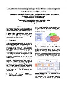
Fig. 1. SPEM 2.0 icons: (a) role denition, (b) work product denition, (c) task denition, (d) role use, (e) work

product use, (f ) task use, and (g) activity.

any new project. However, variability relationships can be more complex than this, e.g., one work product may be considered a satisfactory alternative to another work product. For example, all projects may need a mision denition but for new projects this work product needs to be a comprehensive document while in evolution projects it just needs to dene the project's scope and its relationship with what already exists. Additionally, software process lines manage three types of process elements (tasks, roles and work products), and important variability constraints may involve elements of all three types. The roles that are involved in a project may depend on the amount of resources available and thus the roles responsible for each task may vary. In this paper, we present the variabilities that may appear in software process formal specication. We discuss the available notations and tools, and we make recommendations about them. We illustrate the application of our choice specifying a simple yet interesting requirements engineering process.

2

Modeling Software Process Lines

The Software and Systems Process Engineering Meta-Model (SPEM 2.0) [18] is a standard notation for modeling software and systems development processes and their components. SPEM 2.0 is dened as a UML 2.0 prole, and takes an object-oriented approach to process modeling. SPEM diagrams are used to model two dierent views of a process: a static view, where process components (tasks, work products and roles) are dened; and a dynamic view, where interaction diagrams (like UML activity diagrams) are used to model how process components interact in order to accomplish the goals of the modeled process.

2.1 Process Components One of the goals of using a language like SPEM 2.0 to specify processes is that it gives process engineers mechanisms with which to manage families of processes. In order to encourage process maintenance and reuse, SPEM 2.0 makes a dierence between the denition of process building blocks and their latter use in (possibly more than one) processes. Process components, like tasks, roles and work products, are dened and stored in a Method Library. These denitions can later be reused in multiple process denitions. A process is a collection of activities, where an activity is a big-step grouping of role, work product and task uses. Roles perform activity tasks, and work products serve as input/output artifacts for tasks. The icons for these SPEM 2.0 elements are shown in Figure 1. Roles are used to dene the expected behavior and responsibilities of the team members involved in a process. For example, a role denition like Developer is used to represent team members that will develop parts of the system, and can carry out design, implementation and testing tasks. Note that roles do not represent individual team members, and that one team member may take on several roles at the same time. Also, a single role may be responsible for more than one work product, as well as modify multiple work products. Work products represent anything produced, consumed, or modied by a process. Tangible work products are usually called artifacts, while intangible products are called outcomes. Work products that will be handed o to internal or external parties are also classied as deliverables. Documents, models, repositories, source code and binaries are examples of artifacts and deliverables, while an event like notifying a party that an activity has concluded is an outcome. Formally, roles and work products are stereotyped UML classes,

role

and

work

product, respectively. As such, generalization, aggregation and composition

relationships can be used to dene more complex roles and work products.

2

Fig. 2. SPEM 2.0 task example: Elicit requirements.

Fig. 3. State machine associated to Requirements Document work product.

A task is a set of subtasks/steps that are performed by possibly multiple roles, and involve the creation or modication of one or more work products. Ideally, only one role is responsible for the task. As such, a task denition is a stereotyped class diagram, where the roles that are responsible for it and those that will perform the associated work are identied, as well as the input and output work products (which can be tagged as mandatory or optional). For example, the class diagram in Figure 2 shows the task denition of the typical RE task Elicit requirements. This task denition is associated to two roles: Analyst (responsible) and Client Liaison (performs). This means that a team member with an analyst prole should be in charge of this task, but that we also require somebody from the client's sta to act as stakeholder during the elicitation process. This task has one mandatory output work product, a Requirements Document. Task denitions can also include tool denitions and guidance, but we have omitted these elements for now.

2.2 Process Behavior After having dened the basic process components, we can now specify how work products change state, how tasks are divided into subtasks, and nally, how to put everything together and specify a process (without variability). A work product may go through dierent states during its lifetime. As such, work products can have an associated state model. Process engineers can use this model to specify a work product's states, as well as the permitted transitions between these states. Ideally, such a model can be used to determine how complete a work product is. For example, the state machine for the Requirements Document mentioned in the previous section can be seen in Figure 3. This state machine has three states: initial, validated and approved. The initial state represents an empty document, whereas the validated state indicates that the contents of the document have been validated by both the Analyst and Client Liaison, but the document is not complete. The nal state, approved, is used to indicate that the document is complete and that the Client Liaison has signed o on the document. These work product states can also be used as guards in task denitions. Tasks can be broken down into smaller tasks, modeled using an activity diagram. For example, the task Elicit requirements has three steps: 1) gather requirements, 2) formalize requirements, 3) validate requirements, where there is a feedback loop between validate and gather (shown in Figure 4). In other words, the intended workow for this task is the following: the Analyst meets with the Client Liaison and gathers an initial set of requirements; the Analyst formalizes these requirements (documenting them in the requirements document) and validates them with Client Liaison. This process continues until the Client Liaison is satised with the set of requirements gathered, as well as their formalization. Finally, we can specify a process by using the element denitions we have previously described. Task, role and work product denitions are recommended denitions, we must now specify which denitions will be used in the process. Note that these denitions are only recommendations made by the process engineer, and can be overridden when instantiated, e.g., by adding/removing a work product from a task. Task, role and work product uses are grouped into high-level activities, and a process is a set of these activities, along with

3

Fig. 4. Detailed view of the Elicit requirements task.

Fig. 5. A General Requirements Engineering Process

structural and sequencing information. For example, Figure 5 shows a process model of a general requirements engineering process. It consists of three activities: Exploration, User Requirements Specication & Validation, and Software Requirements Specication & Validation, and a bad result in the nal step may take us back to a previous step. The Elicit Requirements task described before was used in the User Requirements Specication & Validation activity.

3

Modeling Process Variability

It takes a considerable eort to formalize a process in a language like SPEM 2.0, and we do not want re-do this work when formalizing other similar processes. With this in mind, the authors of SPEM 2.0 introduced a set of variability mechanisms, allowing the denition of tailorable processes. In other words, process engineers are expected to dene a common process, and then use the provided variability mechanisms to indicate how to congure the process to individual projects. For example, the General Requirements Engineering Process

4

(a)

(b)

Fig. 6. Simple SPEM 2.0 variability example: (a) congurable model, and (b) a valid conguration of this model.

from Section 2 could be an instantiation of a more general process, where the Exploration activity is only required if the project is set in a new problem domain. In this section, we rst describe the SPEM 2.0 variability mechanism, which provide an indirect manner for specifying variation, and then the vSPEM proposal [16], which focuses on the direct specication of variability, through the denition of variation points and variants.

3.1 SPEM 2.0 Variability Mechanism The SPEM 2.0 standard denes four indirect variability relationships, which must be specied between two variability elements

3 of the same type (e.g., between two work products, between two roles, etc.):

1. Contributes: a source variability element

contributes

its properties to the target variability element

without directly altering any of the target element's properties. In other words, the target element takes on any extra attributes and associations dened by source element, except for those already dened by the target element. 2. Replaces: a source variability element

replaces

its target variability element. In this case, only the

incoming associations of the target element are preserved, both the target's attributes and outgoing associations are replaced by the source element's. The target of multiple

replaces

relations can only

be replaced by one source element in a conguration. 3. Extends: a source variability element

extends the denition of its target variability element, possibly

overriding the target's attributes and associations. 4. Extends-Replaces: in this relationship, a source variability element rst element, and then

replaces

extends its target variability

it.

Instances of these relations may override each other, so variability relations must be resolved in a predetermined order (rst

contributes,

then

replaces,

then

extends

and nally

extends-replaces).

The process tailoring step is successful if the process engineer can resolve away all variability (in a nonconicting manner). A priori, it is hard to predict how variability relations interact with each other, which is why the SPEM 2.0 variability mechanism is classied as indirect. For example, the model in Figure 6a has the following variability relations: the task create UML model contributes to task formalize requirements, work product UML Use Case Model replaces Requirements Document and role UML Modeler extends Analyst, where the formalize requirements task is one of the subtasks of the Elicit Requirements task described in the previous section. In order to remove variability from this model, we must rst resolve the

contributes

relation between the two tasks: task formalize

requirements acquires two outgoing associations, one to UML Modeler and another to UML Use Case Model. The next step is to resolve the

replaces relation between the two work products: UML Use Case

Model replaces Requirements Document in the association with formalize requirements (while keeping

3

In this work, we restrict ourselves to the following variability elements: tasks, roles and work products.

5

(a)

(b)

(c)

(d)

(e)

(f )

(g)

(h)

Fig. 7. (a)  (d) VarPoint icons, and (e)  (h) Variant icons.

(a)

(b)

Fig. 8. Simple vSPEM variability example: (a) congurable model, and (b) a valid conguration of this model.

its own incoming and outgoing associations). Finally, Analyst inherits UML Modeler 's link to UML Use Case Model. The resulting SPEM model (without variability) is shown in Figure 6b. Even in this small model, it was dicult to foresee the results of the tailoring step. Regular process models can get much larger, involving dozens of tasks and even hundreds of work products, so the overall eect of the modeled variability is not always clear. Also, deciding how and where to include variability is a time-consuming, non-replicable and people-dependent process.

3.2 vSPEM Taking into account the limitations of the existing SPEM 2.0 variability mechanisms, Martinez et al. [16] proposed and validated vSPEM, a direct variability mechanism for SPEM 2.0. In this proposal, the process engineer denes process variation points (called

VarPoints ),

as well as variants that can ll the variation

points. In other words, the relationship between a variation point and its variants is a SPEM 2.0

replaces

relation, and during the process tailoring step, each variation point is replaced by exactly one variant (which must be of the same type). Also, variation is now specied at the use level instead of the process component denition level, i.e., activities, role uses, work product uses and task uses are valid variation points. In order to simplify variability modeling, the authors introduced new SPEM icons: the

VarPoint

icons are

shown in Figures 7a  7d, and the variant icons are shown in Figures 7e  7h. In Figure 8a, we show a partial vSPEM specication of the variability modeled in Figure 6a. This model has two variation points, formalize requirements and Requirements Documents, and two variants, formalize requirements using UML and UML Use Case Model. In vSPEM, indirect variability relations, i.e.,

extends-replaces,

contributes, extends

and

are modeled by introducing new variants. For example, the task variant formalize

requirements using UML represents the

contributes

relation in Figure 6a. The tailoring step is now

much simpler: since each variation point in this example has exactly one variant, the tailored model is the one shown in Figure 8b. It is also much clearer in Figure 8b that the nal version of the formalize requirements task includes the creation of a UML model, information that may be obfuscated in a larger SPEM model. According to the empirical studies carried out by the authors in [16], the vSPEM notation was much more intuitive and easy to use than the SPEM 2.0 variability mechanism. Users also found that the results of the process tailoring step were more akin to their idea of the modeled variability when using the new notation. For these reasons, we have adopted this notation in the remainder of this work. In the next section, we discuss possible formalizations of this language.

6

Fig. 9. Example of a basic feature model (from [7]).

4

Formalizing Variability

As discussed in Section 1, the idea of modeling process variability separately from the process denition is quite benecial [2]. In this section, we give an overview of various formalisms currently used in product line analysis [7], and discuss how each one can be used to model vSPEM process variability.

4.1 Basic Feature Models Basic Feature Models [11] (BFM) are frequently used to model variability in product line engineering [8]. In a BFM, features are organized hierarchically, with edges representing parent-child relationships between features. A set of cross-tree constraints is used to indicate relationships between non-directly related features.

Denition 1 (Basic Feature Model). (adapted from [17]) A BFM is a 4-tuple V = (N, E, r, C), where N is a set of nodes representing features, E is a set of edges between nodes, r ∈ N is the single root node representing the domain concept being modeled by the BFM, and C is a set of cross-tree constraints. V is a subset of its nodes. A valid conguration M of a feature model is r ∈ M , M satises the parent-child relationships specied in E , and M also satises constraints dened in C .

A conguration of a BFM conguration such that the cross-tree

BFMs have the following types of edge relationships:

•

Mandatory (man): a mandatory relationship between a parent and child feature means that the child feature must be included in all congurations in which the parent feature appears.

•

Optional (opt): an optional relationship between a parent and child feature means that the child feature can be included in any conguration in which the parent feature appears.

•

Alternative (alt): a set of child features have an alternative relationship with their parent when exactly

•

Or (or ): a set of child features have an or-relationship with their parent when one or more child features

one child feature can be included in any conguration in which the parent feature appears. can be included in any conguration in which the parent feature appears. Thus, an edge respectively) and

e ∈ E is of the form (p, etype, c), where p, c ∈ N (p and c are the parent and child nodes, etype ∈ {man, opt, alt, or}. Figure 9 (from [7]) shows the graphical notation for BFMs.

In this model, Mobile Phone is the root node, which has two optional sub-features (GPS and Media), and two mandatory sub-features (Calls and Screen). Screen is further decomposed using an alternative relation, so a Screen has to be one of the following types:Basic, Color or High resolution; whereas the Media feature is decomposed using an or-relationship, so a Mobile Phone that includes Media can have any of its sub-features.

7

Fig. 10. BFM template for modeling vSPEM variability.

Cross-tree constraints are simple boolean formulas between nodes of the BFM. In this work, we consider the following two types of cross-tree constraints:

• •

V m → Vi=1...k ni , i.e., feature m requires the inclusion of features n1 , n2 . . . nk . Excludes: m → i=1...k ¬ni , i.e., feature m requires the exclusion of features n1 , n2 . . . nk . Requires:

For example, the BFM in Figure 9 has two cross-tree constraints: 1) a requires constraint from Camera to High resolution, indicating that a phone that has a camera

must

have a high resolution screen; and 2) an

excludes constraint between GPS and Basic, indicating that a phone with a basic screen

cannot

have GPS

capabilities, and vice versa. Taking all these constraints into account, this BFM has various valid congurations, like

{Mobile

Phone, Calls, GPS, Screen, High resolution} and

{Mobile

Phone, Calls, Screen, Media,

High resolution, Camera, MP3}.

Modeling vSPEM variability using BFMs.

Since BFMs talk about features, it makes sense to model

both variation points and variants as features. However, since BFMs only identify nodes by label, the modeler must encode the node type (variation point or variant), as well as the variability element type (activity, role use, work product use, or task use) in the node label. Also, since there is no obvious candidate root node, a dummy root node must be added to the BFM (e.g., Variability Prole). Variation points and variants are organized under this root node. We must impose several restrictions on

E

in order to preserve the semantics of vSPEM:

1. vSPEM does not allow nesting of variation points nor variants, which means that the BFM corresponding to a vSPEM variability prole cannot have edges between two features representing variation points (same for variants). 2. In vSPEM, a variant can only be related to a variation point of the same type (e.g., a task use variant can only replace a task use variation point), so the corresponding BFM cannot have edges between features of dierent types. 3. Another condition for producing a valid vSPEM variability prole is that each variation point should be related to at least one variant. 4. In vSPEM, each variation point can only be replaced by one variant once the variability prole has been congured. To ensure this condition, a variation point that has multiple variants should be related to these through an alternative relation. If a variation point has only one variant, this variant is mandatory. 5. Finally, since variation points are variability elements themselves, a variation point can be optional. In Figure 10, we show a basic feature model template for modeling vSPEM variability. Since BFMs only identify nodes by label, it is up to the modeler to manually enforce the additional restrictions on this model, the modeled Variability Prole (root node) has

n

(like VarPoint1 ) or optional (like VarPoint2 ). This prole is also associated to associated to the

n

E.

In

variation points, which can be mandatory

m

variants, which are

variation points through either mandatory or alternative relations, depending on the

amount of variants that a variation point has: a variant is mandatory if it is the only variant associated to a VarPoint (like VarPoint1  in Figure 10); otherwise, variants are alternatives). We have not included cross-tree constraints in Figure 10, but such a BFM can also have cross-tree constraints between its nodes.

Theorem 1. If a BFM meets all the conditions dened above, then all valid congurations of this BFM are valid vSPEM congurations.

8

(a)

(b)

Fig. 11. (a) BFM corresponding to the variability example presented in Section 3, and (b) extending the BFM in (a)

with feature cardinality, indicating that the tailored process requires 12 UML Modelers.

Proof by construction.

t u

For example, the BFM in Figure 11a models the variability example discussed in Section 3. This model has three mandatory variation points: formalize requirements, Requirements Document and Analyst. We have included vSPEM icons in order to visually dierentiate between variation points and variants, as well as labeled the nodes of the model. The formalize requirements variation point is related to two variants: formalize requirements using scenarios and formalize requirements using UML (which appeared in Figure 8a). The Requirements Document node has been similarly decomposed. There is only one possible variant for the Analyst variation point, UML Modeler. This model also has two cross-tree constraints: the task variant formalizing requirements using UML requires the work product UML Use Case Model, which in turn requires a team member that is a UML Modeler. This model has three valid congurations:

{0, 1, 2, 3, 4, 7, 8}. M1

M1 = {0, 1, 2, 3, 5, 7, 8}, M2 = {0, 1, 2, 3, 4, 6, 8},

and

M3 =

represents the conguration where the variant formalizing requirements using UML

is selected, which means that variants UML Use Case Model and UML Modeler must also be selected, because of the cross-tree constraints. On the other hand, if the variant formalizing requirements using scenarios is selected, both variants for Requirements Document are valid, corresponding to congurations

M2

and

M3 .

The variant UML Modeler is present in all congurations because it is a mandatory variant.

4.2 Cardinality-based Feature Models Cardinality-based Feature Models [9] (CFM) are an extension to BFMs, where UML-like multiplicities (socalled

•

cardinalities ) have been added to certain elements of the model:

Feature cardinality ([m..n]): used to indicate the number of instances of the feature that can be part of the nal conguration, where

•

Group cardinality (
):

and

n

are the lower and upper bounds, respectively.

used to indicate the number of child features that can be selected when

its parent feature is selected, where

m

and

n

are the lower and upper bounds, respectively.

Figure 11b shows how feature cardinality was added to a part of the BFM in Figure 11a. By adding the feature cardinality

[1..2]

to UML Modeler, we are indicating that the tailored process requires one to two

team members that meet the UML Modeler prole. Group cardinality aects alternative and or-relationships. In our translation of vSPEM to BFM, we only used the alternative relation, in order to model the relationship between a parent variation point and its children variants (modeling that just one variant may be selected per variation point). Thus, we do not have any use for this modeling concept.

9

Fig. 12. Using feature attributes to expand the information available about the Analyst node.

Fig. 13. Example of an orthogonal variability model (from [23]).

4.3 Extended Feature Models Extended Feature Models [11] (EFM) are an extension to BFMs, where additional information about features is available. This is usually accomplished by adding feature attributes [12, 5, 6]. There is no consensus on a notation to dene attributes. However, most proposals agree that an attribute should at least have a name, domain and value. For example, Figure 12 shows an example of how feature attributes can be used to better document the nodes of the BFM in Figure 11a. Instead of informally adding extra labels and icons, the Analyst node now has three attributes, featureType, id and elementType, where FeatureTypes ={root, VarPoint, Variant } and ElementTypes = {Activity, Role Use, Work Product Use, Task Use }.

4.4 Orthogonal Variability Model Orthogonal Variability Models [20, 19] (OVM) is another notation used to model product line variability. The main dierence between OVMs and feature models is that OVMs only document the variabilities present in a product line, whereas feature models model both the common aspects of a product line and its variability. Thus, OVM elements are either variation points or variants: variation points indicate elements that may vary, while variants represent dierent possible realizations of a variation point. Each variation point must be related to a least one variant, which is called a dependency in OVM (and corresponds to the BFM concept of relations). OVM denes three types of dependencies: mandatory, optional, and alternative, which are interpreted just like their BFM counterparts. Group cardinalities can be dened for alternative dependencies. Additionally, each variant must be related to one and only one variation point. Finally, OVMs also allow requires and excludes constraints between modeled elements, these can be dened between two variants or two variation points, or between a variation point and a non-dependent variant. Another dierence with feature models is that OVMs elements are not hierarchical, since each variation point is orthogonal to the rest (hence the name of the modeling notation); however, this hierarchy can be modeled using constraints. Figure 13 (from [23]) shows the graphical notation for OVMs. In this variability model of a cellular phone product line, Messaging, Utility Functions and OS are three mandatory variation points.In this example, the variation point Messaging has two variants, SMS and MMS, related through an alternative dependency relation with a

[1..2] cardinality. This means that valid congurations of this model must contain 10

Fig. 14. OVM corresponding to the variability example presented in Section 3.

at least one of the two variants (or both). The OS variation point has a similar decomposition using an alternative relation, but no cardinality is explicitly modeled. This means that the default

[1..1]

cardinality

applies to this relation and valid congurations of this model must contain exactly one variant associated to the OS node. The Utility Functions variation point has two optional dependents, valid congurations of this model can contain none, one or both of the related variants. Finally, there is a requires constraint from Currency Exchange to Calculator, indicating that valid congurations of the model that include Currency Exchange must also include a Calculator. Just like feature models, we can talk about valid OVM congurations. A valid conguration of an OVM is a subset of its variants such that its dependencies and constraints are satised

Modeling vSPEM variability using OVMs. vSPEM and OVMs have similar modeling constructs and semantics, so the mapping from vSPEM to OVM is direct. The main dierence between the two is that vSPEM does not allow general group cardinalities on alternatives, so we must restrict ourselves to OVM without cardinalities when modeling vSPEM variability. Figure 14 shows an OVM that models the variability example discussed in Section 3. This model is equivalent to the BFM version in Figure 11a, since there is a one-to-one mapping between the valid congurations of both models. This is because there is a one-to-one mapping between the modeled elements (except for the dummy root feature) and equivalent constraints exist in both models. This result was not surprising, as it conrms the results obtained by Roos-Frantz et al. [23]. In [23], the authors present a BFM to OVM translation algorithm, indicating specic cases were special care needed to be taken in order to preserve the semantics of the original BFM. Since we used a reduced subset of BFM to represent vSPEM variability, we did not encounter the problems described in [23], and there is a direct mapping between a BFM and an OVM modeled using our restricted subsets of these notations.

4.5 Discussion As discussed in the previous section, the SPEM standard advocates for a single process model that includes variability, whereas vSPEM focuses on a separate specication of common and variable process elements. Empirical studies [16] seem to favor the latter approach, so in this section, we studied how to formalize vSPEM variability using popular product line formalisms: dierent types of feature models (Sections 4.1  4.3) and orthogonal variability models (Section 4.4). We found that we did not need the full expressiveness of feature models to formalize vSPEM, since this notation only focuses on variability. We also found that we could directly formalize vSPEM using OVM, since both notations share core concepts. Finally, we found that there is a direct mapping between a FM representing vSPEM variability and the corresponding OVM, a conclusion supported by the results in [23]. Thus, the decision about which formalism to use comes down to a question of available tool support, which we discuss in the next section.

11

5

Tool Support for Feature Models and Orthogonal Variability Models

The main advantage of formalizing models is that we can analyze these models using automated techniques. For example, by mapping a feature model into a propositional formula [17], an o-the-shelf SAT solver can be used to determine whether a feature model is consistent or not (i.e., it has at least one valid conguration), or whether a given conguration is a valid. By formalizing variability, we can apply these same analyses to variability models. For example, we can check that the modeled variability is consistent, and also determine valid congurations that can be used to automatically tailor the corresponding process. A more complete list of feature model analysis operations, as well as dierent underlying formalisms, can be found in [7]. On the other hand, the analysis of orthogonal variability models has up till recently been done in an ad-hoc manner [19], but recent work [22] has focused on the use of constaint programming to analyze OVMs. In this section, we give an overview of various publicly available FM and OVM analysis tools.

5.1 fmp The Feature Modeling Plug-in (fmp) [15] is an Eclipse plug-in for editing and conguring cardinality-based feature models. Fmp can be used standalone in Eclipse or together with fmp2rsm plug-in in Rational Software Modeler (RSM) or Rational Software Architect (RSA). fmp2rsm integrates fmp with RSM and enables product line modeling in UML. This tool is mainly used to check feature model consistency, as well as to generate valid congurations and to check the validity of partial congurations. The project has been completed, so the tool is no longer maintained by its original developers; however, the project is now opensource, and the code is available on SourceForge.

5.2 Clafer Clafer (

class, feature, reference) [4] is a concept modeling language for specication and analysis of software

product lines. Clafer provides rst-class support for feature modeling, including feature modeling extensions like cardinality-based feature modeling. The authors have developed a rst version of a Clafer to Alloy [10], which enables model analysis through the use of the Alloy Analyzer. The Alloy Analyzer supports various analyses, like checking model consistency and generating valid congurations. The authors also provide a SPLOT (see next subsection) to Clafer translator, as well as a Clafer parser in Java. These tools are available at [14].

5.3 SPLOT SPLOT (Software Product Lines Online Tools) [13] is a collection of interactive online tools for editing, conguring, and analysing feature models. SPLOT is also a feature model repository. SPLOT supports basic feature models (i.e., no cardinality) and oers basic model analyses, like those described at the beginning of this section, as well as some more advanced analyses like nding the number of common and dead features (common features appear in every model conguration, while dead features do not appear in any congurations).

5.4 FaMa-OVM FaMa-OVM[22] provides automated analyses for orthogonal variability models. This tool oers basic analyses, like checking consistency and generating valid congurations, but also focuses on verifying user-specied quality conditions, allowing the generation of an optimal conguration as well as the most representative one. This tool is still in the prototype stage, and is available at [21].

12

6

Summary and Conclusions

Software process lines (SPrL) are families of related processes, built from a set of administrated software process elements in a preestablished fashion, similar to how software product lines (SPL) are built with software assets. In SPLs, variability is usually specied using feature models and orthogonal variability models. In this paper, we explored the feasibility of using these modeling formalisms for specifying SPrL variability, using a simple requirements engineering process as a running example. Process line variability can be specied in two ways: 1) using the SPEM 2.0 variability mechanisms, which provide an indirect manner for specifying variation, and 2) using the vSPEM, which focuses on the direct specication of variability, through the denition of variation points and variants. As discussed in Section 3, we focused on the vSPEM notation for modeling process variability, where variability is modeled separately from the process denition. The reason for this choice is that vSPEM is more intuitive and easy to use in practice [16]. We studied how to formalize vSPEM variability using popular product line formalisms: dierent types of feature models (Sections 4.1  4.3) and orthogonal variability models (Section 4.4). The main results of this report is that both feature models and orthogonal variability models can be used to formalize vSPEM process variability, and that we did not need to use the full expressiveness of either formalism to do it. Also, cardinality may be useful in the specication of variability, but we must study more examples to determine whether it is really needed. Thus, the decision about which formalism to use comes down to a question of available tool support. The surveyed tools all oered two basic analyses: checking whether a model is consistent (i.e., it has at least one valid conguration) and generating valid congurations. If we need to model cardinality, then we have to use tools that support CFMs, like fmp or Clafer. Otherwise, SPLOT and FaMa-OVM oered additional analyses that may be interesting in practice. Finally, in order to better understand variability and its formalization, we propose to carry out a more extensive case study. This will allow us to get a better sense of what kinds of variability exist in-the-wild, which will give us a better idea of how expressive the underlying formalism needs to be in practice, and what types of automated analyses are available.

References 1. Julio Ariel Hurtado Alegria, M. Cecilia Bastarrica, and Alexandre Bergel. Analyzing Software Process Models with AVISPA. In International Conference on Software and Systems Processes, ICSSP 2011, Hawaii, USA, May 21-22, 2011. Proceedings. ACM, 2011. Accepted for publication.

2. Julio Ariel Hurtado Alegria, M. Cecilia Bastarrica, Alcides Quispe, and Sergio F. Ochoa. An MDE Approach to Software Process Tailoring.

In International Conference on Software and Systems Processes, ICSSP 2011,

Hawaii, USA, May 21-22, 2011. Proceedings. ACM, 2011. Accepted for publication.

3. Julio Ariel Hurtado Alegria, Alejandro Lagos, Alexandre Bergel, and M. Cecilia Bastarrica. Software Process Model Blueprints. In Jürgen Münch, Ye Yang, and Wilhelm Schäfer, editors, New Modeling Concepts for Today's Software Processes, International Conference on Software Process, ICSP 2010, Paderborn, Germany, July 8-9, 2010. Proceedings, volume 6195 of Lecture Notes in Computer Science, pages 273284. Springer, 2010.

4. Kacper B¡k, Krzysztof Czarnecki, and Andrzej W¡sowski. Feature and Meta-Models in Clafer: Mixed, Specialized, and Coupled. In 3rd International Conference on Software Language Engineering, Eindhoven, The Netherlands, 10/2010 2010. 5. Don S. Batory. Feature Models, Grammars, and Propositional Formulas. In Software Product Lines, 9th International Conference, SPLC 2005, Rennes, France, September 26-29, 2005, Proceedings, pages 720, 2005.

6. Don S. Batory, David Benavides, and Antonio Ruiz Cortés. Automated analysis of feature models: challenges ahead. Commun. ACM, 49(12):4547, 2006. 7. David Benavides, Sergio Segura, and Antonio Ruiz Cortés. Automated analysis of feature models 20 years later: A literature review. Inf. Syst., 35(6):615636, 2010. 8. Paul Clements and Linda Northrop. Software Product Lines: Practices and Patterns. Addison-Wesley Professional, third edition, August 2001.

13

9. Krzysztof Czarnecki, Simon Helsen, and Ulrich W. Eisenecker. Formalizing cardinality-based feature models and their specialization. Software Process: Improvement and Practice, 10(1):729, 2005. 10. Daniel Jackson. Software Abstractions: Logic, Language, and Analysis. The MIT Press, 2006. 11. Kyo C. Kang, Sholom G. Cohen, James A. Hess, William E. Novak, and A. Spencer Peterson. Feature-oriented domain analysis (foda) feasibility study.

Technical Report CMU/SEI-90-TR-21, Carnegie Mellon University,

November 1990. 12. Kyo C. Kang, Sajoong Kim, Jaejoon Lee, Kijoo Kim, Euiseob Shin, and Moonhang Huh. FORM: A featureoriented reuse method with domain-specic reference architectures. Ann. Softw. Eng., 5:143168, January 1998. 13. Computer Systems Group / Generative Software Development Lab.

SPLOT - Software Product Line Online

Tools. http://www.splot-research.org/, Accessed September 2011. 14. Generative Software Development Lab. Clafer. http://gsd.uwaterloo.ca/clafer, Accessed September 2011. 15. Generative

Software

Development

Lab.

Feature

Modeling

and

Model

Templates.

http://gsd.uwaterloo.ca/featureModelingAndModelTemplates, Accessed September 2011. 16. Tomás Martínez-Ruiz, Félix García, Mario Piattini, and Jürgen Münch. Modelling software process variability: an empirical study. IET Software, 5(2):172187, 2011. 17. Marcílio Mendonça, Andrzej Wasowski, and Krzysztof Czarnecki. SAT-based Analysis of Feature Models is Easy. In Software Product Lines, 13th International Conference, SPLC 2009, San Francisco, California, USA, August 24-28, 2009, Proceedings, pages 231240, 2009.

18. OMG.

Software

and

Systems

Process

Engineering

Metamodel

specication

(SPEM)

Version

2.0.

http://www.omg.org/spec/SPEM/2.0, Accessed June 2011. 19. Klaus Pohl, Günter Böckle, and Frank J. van der Linden.

Software Product Line Engineering: Foundations,

Principles and Techniques. Springer, November 2010.

20. Klaus Pohl, Frank van der Linden, and Andreas Metzger. Software Product Line Variability Management. In Software Product Lines, 10th International Conference, SPLC 2006, Baltimore, Maryland, USA, August 21-24, 2006, Proceedings, page 219, 2006.

21. Fabricia Roos-Frantz, David Benavides, A. Ruiz-Cortés, André Heuer, and Kim Lauenroth.

Complementary

material. http://www.lsi.us.es/ dbc/material/SofQualJ11/, Accessed September 2011. 22. Fabricia Roos-Frantz, David Benavides, A. Ruiz-Cortés, André Heuer, and Kim Lauenroth. Quality-aware analysis in product line engineering with the orthogonal variability model.

Software Quality Journal Special Issue on

Quality Engineering for Software Product Lines, 2011.

23. Fabricia Roos-Frantz, David Benavides, and Antonio Ruiz-Cortés. Feature Model to Orthogonal Variability Model Transformations. A First Step. Actas de los Talleres de las Jornadas de Ing. de Software y BBDD, 3(2):8190, 2009.

14