Modelling and numerical/experimental investigation ...

NATIONAL TECHNICAL UNIVERSITY OF ATHENS SCHOOL OF NAVAL ARCHITECTURE AND MARINE ENGINEERING

Modelling and numerical/experimental investigation of granular cargo shift in maritime transportation

by

Christos C. Spandonidis

Doctoral Thesis

Athens, August 2016

NATIONAL TECHNICAL UNIVERSITY OF ATHENS SCHOOL OF NAVAL ARCHITECTURE AND MARINE ENGINEERING

Modelling and numerical/experimental investigation of granular cargo shift in maritime transportation

by

Christos C. Spandonidis

A dissertation submitted in partial fulfilment of the requirements for the degree of Doctor of Philosophy

Advisory Committee: Konstantinos J. Spyrou, Professor (Supervisor) Gerassimos A. Athanassoulis, Professor Apostolos D. Papanikolaou, Professor

Athens, August 2016

This thesis is dedicated to the three precious women in my life: my wife, my daughter and my mother. Also to my father.

Abstract The study of granular materials (powders, sands, grains, metal ore etc.) should be a topic of great interest in naval architecture, since cargo shift represents a major hazard for ship safety and probably the most common cause of capsize of large ships. Despite though its great importance, the behaviour of granular cargos transported by sea has not been sufficiently investigated yet from a theoretical perspective. As a result, international regulations governing the procedures of loading and stowage of bulky cargos, while continuously updated and improved, remain mainly empirical. In the current Thesis, a micro-scale modelling approach is presented, aimed to develop capability for simulating the dynamic behaviour of granular materials having physical properties conforming to those of bulky cargos commonly transported through the sea, inside ship holds. The well-established method of “Molecular Dynamics” is employed for modelling particles’ interactions and for predicting macroscopic features of the excited granular material behaviour. The algorithm is further combined with standard models of ship motion, in order to understand the interplay of granular material flow with vessel motion. At the first stage, “dry” granular materials comprised of spherical particle and affected by non-linear frictional forces are employed. Later, a number of improvements are incorporated, to bring the model closer to reality, by introducing the effect of environmental humidity and also the irregularity in particles’ shape. To discern qualitatively different patterns of behaviour, a variety of materials and filling ratios have been examined. Moreover, to improve performance, the computational algorithm was parallelized for Graphical Processing Unit (GPU) implementation and the merit of it was properly evaluated. Characteristic simulation results of a 2D rectangular scaled barge, partly filled with bulky cargo and vibrated in roll, sway and heave are included in the Thesis. The barge is, either, forced to oscillate in a prescribed motion; or is free to move under the effect of wave loads and her cargo’s occasional fluid-like movement. Critical parameter values where cargo shift is initiated are identified. The intention has been to maintain the excitation amplitudes and frequencies close to realistic open sea conditions although the scaling problem is in itself a major scientific challenge. Judging from the qualitative character of the obtained results and also from comparisons of some key findings with experimental results, it appears that the described simulation model has good potential to evolve into a useful and practical computational tool for the investigation of stability of ships carrying solid cargos in bulky form.

Keywords: granular material, molecular dynamics, cargo shift, ship stability, capsize

Table of Contents Abstract ............................................................................................................................................... v Table of Contents .............................................................................................................................. vii List of Figures .................................................................................................................................... xi List of Tables .................................................................................................................................... xvi Chapter 1: Introduction ................................................................................................................... 17 1.1

General framework and aim of research.............................................................................. 17

1.2

Focal points of interest ........................................................................................................ 19

1.3

Need for further research..................................................................................................... 20

1.4

Methodology ....................................................................................................................... 21

1.5

Contributions of the thesis................................................................................................... 21

1.6

Thesis outline ...................................................................................................................... 22

Chapter 2: Critical literature review ............................................................................................... 25 2.1

Granular nature ................................................................................................................... 25

2.2

IMO bulk cargo regulation review ...................................................................................... 27

2.3

Granular materials behaviour .............................................................................................. 27

2.4

Research approaches for investigating granular materials ................................................... 28 Granular material modelling approaches ..................................................................... 30

2.4.1 2.5

Angle of repose ................................................................................................................... 33

2.6

Behaviour of granular material under prescribed vibration ................................................. 36

2.6.1

Vertical (heave) vibration ............................................................................................ 36

2.6.2

Lateral (sway) vibration .............................................................................................. 39

2.7

Coupled ship-cargo motion ................................................................................................. 39

2.8

“Weakly wet” granular materials ........................................................................................ 39

2.9

Granular material behaviour computing in Graphical Processing Unit ............................... 42

2.10

Non-spherical particle research ........................................................................................... 43

2.10.1

Non-spherical DEM approaches.................................................................................. 45

2.10.2

Realistic shape descriptors .......................................................................................... 48

Chapter 3: Objectives ....................................................................................................................... 51 Chapter 4: Basic Mathematical Model............................................................................................ 53 4.1

Molecular Dynamics simulation ......................................................................................... 53

4.1.1

Coupled ship-cargo motion implementation................................................................ 54

vii

Interaction forces................................................................................................................. 56

4.2

4.2.1

Dry granular solids and aggregates ............................................................................. 56

4.2.2

Implementation of humidity ........................................................................................ 59

4.3

Systems of coordinates ........................................................................................................ 60

4.4

Model verification ............................................................................................................... 61

4.5

Validation............................................................................................................................ 62

Chapter 5: Granular Flow under Prescribed Tank Motion .......................................................... 65 5.1

System Definition ............................................................................................................... 65

5.2

Dependence of granular flow on particle’s properties ......................................................... 66

5.2.1

Slow tilting of tank – identification of angle of repose................................................ 67

5.2.2

Motion under horizontal (sway) and vertical (heave) excitation.................................. 69

5.3

Dependence of granular flow on system’s configuration .................................................... 74

5.3.1

Dependence of angle of repose on initial free surface configuration ........................... 75

5.3.2

Dependence of angle of repose on side wall height ..................................................... 78

5.3.3

Slow tilting of tanks with different filling ................................................................... 79

5.3.4

Investigation of material’s hysteretic behaviour .......................................................... 82

5.3.5

Granular material flow depending on the position of the roll centre............................ 83

5.4

Scaling effects ..................................................................................................................... 86

5.4.1

Horizontal motion under sway excitation .................................................................... 87

5.4.2

Slow tilting of the tank – identification of angle of repose .......................................... 89 Concluding remarks ............................................................................................................ 90

5.5

Chapter 6: Code Parallelization in CUDA Environment............................................................... 93 6.1

Implementation ................................................................................................................... 93

6.2

Numerical verification/validation of the algorithm ............................................................. 95

6.3

Performance results ............................................................................................................. 98

6.4

Discussion ......................................................................................................................... 100

6.5

Concluding remarks .......................................................................................................... 101

Chapter 7: Coupled ship - cargo motion in regular beam seas ................................................... 103 7.1

System definition .............................................................................................................. 103

7.2

Single Degree of Freedom - Roll....................................................................................... 104

7.2.1

Equation of motion.................................................................................................... 104

7.2.2

Case study ................................................................................................................. 107

7.3

Three degrees of Freedom (Roll - Sway - Heave) ............................................................. 113

7.3.1

viii

Equations of motion .................................................................................................. 113

7.3.2

Dry cargo .................................................................................................................. 115

7.3.3

Implementation of humidity ...................................................................................... 120


7.4

Chapter 8: Cargo with Irregularly-Shaped Particles................................................................... 125 Methodology description .................................................................................................. 125

8.1

8.1.1

Object generation ...................................................................................................... 125

8.1.2

Contact detection ....................................................................................................... 129

8.1.3

Physics and visualisation ........................................................................................... 131

Validation results and discussion ...................................................................................... 132

8.2

8.2.1

Investigation of semi-static behaviour: angle of repose............................................. 132

8.2.2

Dynamic behaviour – sway oscillation ...................................................................... 133

8.2.3

Coupled fluid-ship-material motion in 3 DOF........................................................... 135

8.2.4

Discussion ................................................................................................................. 136

8.3

Numerical experiments with irregularly - shaped particles ............................................... 136

8.3.1

Dependence of the angle of repose upon the Fourier Descriptors.............................. 137

8.3.2

Dependence of angle of repose on phase angle distribution ...................................... 139

8.3.3

Shipboard test method ............................................................................................... 141

8.4


Chapter 9: Experimental reproduction of key results ................................................................. 143 9.1

Experimental Setup ........................................................................................................... 143

9.2

Evaluation of qualitative efficiency of simulations ........................................................... 144

9.2.1

Response of granular material under slow tilting ...................................................... 145

9.2.2

Scaling effects ........................................................................................................... 146

9.2.3

Different filling ratios and tilting rates ...................................................................... 147

9.3

Evaluation of simulation results’ accuracy ........................................................................ 149

9.4

Experimental investigation of cargo liquefaction .............................................................. 152

9.4.1

Results for sand ......................................................................................................... 153

9.4.2

Results for olive pomace ........................................................................................... 154

9.5


Chapter 10: Conclusions ................................................................................................................ 157 10.1

General overview .............................................................................................................. 157

10.2

Outcome of investigation .................................................................................................. 158

10.3

Discussion ......................................................................................................................... 161

10.4

Future work ....................................................................................................................... 162

ix

References........................................................................................................................................ 165 Appendix A: General Purpose Graphical Processing Unit Architecture .................................. 181 Α.1 CUDA and the NVIDIA GeForce GTX Architecture ............................................................ 181 A.2 THRUST library .................................................................................................................... 183 Appendix B: Trajectory Generation for the 2D case................................................................... 185 Appendix C: Scaling technique ..................................................................................................... 189 Appendix D: Investigation of angle of repose using the shipboard test method........................ 193 D.1 System description ................................................................................................................. 193 D.2 Comparison with tilting box test ............................................................................................ 197 D.3 Concluding remarks ............................................................................................................... 198 Appendix E: Coupled ship-cargo 3 DOF equations of motion ................................................... 199 Appendix F: Initialisation of wave propagation .......................................................................... 205

x

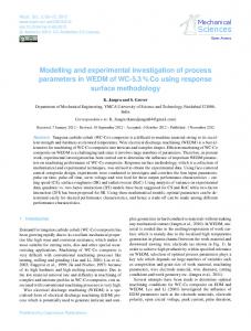
List of Figures FIGURE 1.1 ABOUT 15% OF SHIP LOSSES (LEFT) AND 40.0% OF THE TOTAL LOSS OF LIFE (RIGHT), ASSOCIATED WITH BULK-CARRIER SHIPS, OVER THE PERIOD 2005 – 2015, HAVE BEEN ATTRIBUTED TO A CARGO RELATED CAUSE AND MAINLY TO LIQUEFACTION (INTECARGO 2016). .................................................................................................................................. 18 FIGURE 2.1 GRANULAR MATTER ON MICROSCOPE. LEFT: SAND, RIGHT: OLIVE POMACE. DIFFERENT GRAIN SIZES, SHAPES AND EVEN MATERIAL ARE FORMING THE ACTUAL MATERIAL. .................................................................................................. 25 FIGURE 2.2 SCHEMATIC AND PHYSICAL DESCRIPTION OF MATERIAL STATE BASED ON ITS LIQUID CONTENT (SOURCE: MITARAI & NORI 2006). ...................................................................................................................................................... 40 FIGURE 2.3 GRAPHICAL REPRESENTATION OF THE MAJOR NON-SPHERICAL DEM APPROACHES: A) ELLIPTICAL, B) SUPER QUADRIC C) POLYGON, D) DISCRETE FUNCTION REPRESENTATION AND E) MULTI-ELEMENT METHOD................................................. 44 FIGURE 2.4 M-R PLOTS FOR SINGLE FRACTAL ELEMENT (LEFT) AND SEDIMENTARY PARTICLE USING MULTIPLE FRACTAL ELEMENTS (RIGHT). (SOURCES: A) ORFORD & WHALLEY 1983, B) KENNEDY & LIN, 1992). ........................................................ 50 FIGURE 4.1 MOLECULAR DYNAMICS SIMULATION ......................................................................................................... 53 FIGURE 4.2 MOLECULAR DYNAMICS’S PROCESSING STEP FOR THE CASE OF COUPLED SHIP-CARGO SIMULATION. .......................... 55 FIGURE 4.3 GRAINS PENETRATION. ........................................................................................................................... 56 FIGURE 4.4 PARTICLE CONDITION AFTER COLLISION (SOURCE; RICHEFEU ET AL 2006). .......................................................... 59 FIGURE 4.5 THE THREE DIFFERENT COORDINATE SYSTEMS (SOLID LINES) AND THEIR IRROTATIONAL EQUIVALENTS (DASHED LINES) ARE BEING DEPICTED............................................................................................................................................ 61 FIGURE 4.6 COMPARISON OF SIMULATION RESULTS TO EXPERIMENTAL DATA WHEN A TWO DIMENSIONAL STACK IS IN GUIDED FALL. 62 FIGURE 4.7 COMPARISON OF SIMULATION RESULTS TO EXPERIMENTAL DATA. TESTING OF GRANULAR MATTER INVOLVING HORIZONTAL SHAKING, FOR VARIOUS FILLING HEIGHTS IN TANK. ................................................................................................ 63 FIGURE 5.1 DIFFERENT TIME INSTANTS OF THE SLOWLY TILTED TANK, FOR MATERIAL A (LEFT), B (MIDDLE) AND C (RIGHT) IN THE CASE ST OF THE 1 TANK CONFIGURATION. UP: TANKS AT THE BEGINNING OF THE TEST (0 S). DOWN: TANKS’ STATE WHEN THE FREE SURFACE GRANULES BEGIN TO FLOW (AT 6 S, 5.5 S AND 3.9 S, FROM LEFT TO RIGHT).................................................... 67 FIGURE 5.2 SNAPSHOTS OF THE STATE OF THE TANKS AS THE TILTING PROGRESSES. DIFFERENT TIME INSTANTS OF TANK TILTING, FOR ND MATERIAL A, B AND C IN THE CASE OF THE 2 TANK CONFIGURATION. ...................................................................... 68 FIGURE 5.3 STEADY OSCILLATION AMPLITUDE OF MASS CENTRE UNDER HORIZONTAL OSCILLATION............................................ 69 FIGURE 5.4 HORIZONTAL (LEFT) AND VERTICAL (RIGHT) MOVEMENT OF CENTRE OF MASS OF MATERIAL A (RED), B (GREEN) AND C (BLUE), UNDER SWAY OSCILLATION WITH TWO DIFFERENT EXCITATION FREQUENCIES: I) 0.2 HZ (DASHED LINE), II) 1.5 HZ (SOLID LINE). TANK WIDTH IS 19.2CM. ........................................................................................................................ 70 FIGURE 5.5 TIME INSTANTS OF MOTION OF MATERIAL B, FOR EXCITATION FREQUENCY 1.5 HZ (HORIZONTAL). LEFT: BEGINNING OF THE MOTION. MIDDLE: TIME INSTANT BETWEEN THE BEGINNING AND THE INSTANT OF MAXIMUM AMPLITUDE. RIGHT: INSTANT RIGHT AFTER THE MAXIMUM AMPLITUDE IS REACHED AND THE TANK MOVES TO THE LEFT FOR THE FIRST TIME. .................... 70 FIGURE 5.6 HORIZONTAL (LEFT) AND VERTICAL (RIGHT) MOVEMENT OF CENTRE OF MASS OF MATERIAL A (RED), B (GREEN) AND C (BLUE), UNDER VERTICAL OSCILLATION IN TWO DIFFERENT EXCITATION FREQUENCIES: I) 0.2 HZ (DASHED LINE), II) 1.5 HZ (SOLID LINE). THE TANK WIDTH IS FIXED.............................................................................................................. 71 FIGURE 5.7 HORIZONTAL (LEFT) AND VERTICAL (RIGHT) MOVEMENT OF CENTRE OF MASS OF MATERIAL A (RED), B (GREEN) AND C (BLUE) UNDER SWAY OSCILLATION IN TWO DIFFERENT EXCITATION FREQUENCIES: I) 0.2 HZ (DASHED LINE), II) 1.5 HZ (SOLID LINE). TANK’S HEIGHT TO WIDTH RATIO VALUE IS FIXED. ......................................................................................... 72 FIGURE 5.8 STEADY OSCILLATION AMPLITUDE OF CENTRE OF MASS UNDER HORIZONTAL HARMONIC EXCITATION.......................... 72 FIGURE 5.9 STATUS OF PARTICLES OF MATERIAL B UNDER HORIZONTAL HARMONIC EXCITATION WITH FREQUENCY 1.5 HZ. LEFT: BEGINNING OF THE MOTION. MIDDLE: TIME INSTANT BETWEEN THE BEGINNING AND THE INSTANT OF MAXIMUM AMPLITUDE. RIGHT: INSTANT WHEN THE MAXIMUM AMPLITUDE IS REACHED FOR THE FIRST TIME. .................................................... 72 FIGURE 5.10 BEHAVIOUR OF B MATERIAL’S CENTRE OF MASS, FOR THE TWO TANK CONFIGURATIONS (HORIZONTAL VIBRATION, F = 1.5 HZ). THE PHASE BETWEEN RESPONSE AND EXCITATION APPEARS TO BE ALMOST 180°. ............................................. 73 FIGURE 5.11 HORIZONTAL (LEFT) AND VERTICAL (RIGHT) MOVEMENT OF MASS CENTRE FOR MATERIAL A (RED), B (GREEN) AND C (BLUE) UNDER VERTICAL (HEAVE) HARMONIC EXCITATION WITH FREQUENCY: 0.2 HZ (DASHED LINE); 1.5 HZ (SOLID LINE). THE NUMBER OF PARTICLES IS THE SAME WHILE TANKS ARE SCALED TO PARTICLE SIZE. ......................................................... 73

xi

FIGURE 5.12 THREE DIFFERENT INITIAL FREE SURFACE CONFIGURATIONS: A) UNDISTURBED FREE SURFACE (LEFT), B) SLIGHTLY DISTURBED FREE SURFACE (MIDDLE) AND C) DISTURBED FREE SURFACE (RIGHT). ........................................................... 75 FIGURE 5.13 DISPLACEMENT OF B MATERIAL’S CENTRE OF MASS, FOR TILTING RATE 0.3°/S. COMPARATIVE STUDY FOR THREE DIFFERENT INITIALIZATIONS. SUFFICIENTLY HIGH TANK WALLS ARE ASSUMED. .............................................................. 75 FIGURE 5.14 DISPLACEMENT OF B MATERIAL’S CENTRE OF MASS, FOR DIFFERENT TILTING RATES WHEN THE FREE SURFACE IS A) SLIGHTLY DISTURBED (UPPER), B) ABSOLUTELY UNDISTURBED (LOWER). ..................................................................... 76 FIGURE 5.15 SNAPSHOTS OF B MATERIAL PARTICLES DURING TILTING, WITH RATE OF ROTATION 3°/S, FOR TWO DIFFERENT CASES: A) TANK WITH SUFFICIENTLY HIGH-SIDED WALLS (LEFT), B) TANK WITH SIDE WALL HEIGHT EQUAL TO MATERIAL’S HEIGHT (RIGHT). ................................................................................................................................................................ 77 FIGURE 5.16 BEHAVIOUR OF THE PARTICLES DURING TILTING WITH RATE 0.3°/S IN THE LOW-SIDED TANK, MONITORED BY TWO DIFFERENT MACROSCOPIC INDICES: A) DISPLACEMENT OF CENTRE OF MASS (LEFT) B) RATIO OF PARTICLES LEAVING THE TANK TO TOTAL NUMBER OF FREE - TO - MOVE PARTICLES (RIGHT). ....................................................................................... 78 FIGURE 5.17 THREE SIMILAR TANKS WERE USED FOR THE NUMERICAL EXPERIMENTS. WHILE THE TANK LENGTH IS THE SAME, MATERIAL’S HEIGHT INSIDE THE TANK IS VARIED, LEADING THUS TO DIFFERENT FILLING RATIOS. ........................................ 79 FIGURE 5.18 MASS CENTRE DISPLACEMENT FOR THE THREE TANKS, UNDER DIFFERENT TILTING RATES: A) 1 DEG/S, B) 0.5 DEG/S, C) 0.3 DEG/S................................................................................................................................................... 80 FIGURE 5.19 HYSTERETIC BEHAVIOUR OF MATERIAL INSIDE TANK A (LEFT) AND B (RIGHT) ...................................................... 82 FIGURE 5.20 TIME SHOTS FROM FINAL MATERIAL POSITION AFTER REVERSE MOTION WITH TILTING RATE -1 DEG/S. ..................... 82 FIGURE 5.21 MASS CENTRE’S DISPLACEMENT IN TANK A FOR 1 DEG/S TILTING RATE. THE TANK ALTERS ITS TILTING RATE FROM ANTICLOCKWISE TO CLOCKWISE RIGHT AFTER MATERIAL COLLAPSE OCCURS. IT IS SHOWN THAT DESPITE THE OPPOSITE ROTATIONAL MOTION, MATERIAL INSIDE THE TANK SETTLED TO ITS FINAL POSITION AFTER THE COLLAPSE............................ 83 FIGURE 5.22 INITIAL SEPERATED MATERIAL PART. ......................................................................................................... 83 FIGURE 5.23 DISPLACEMENT OF MATERIAL’S CENTRE OF MASS, FOR VARIOUS ROLL CENTRES. THE EXCITATION FREQUENCY IS 1.3 HZ AND THE AMPLITUDE IS 20 DEG. ....................................................................................................................... 84 FIGURE 5.24 MATERIAL’S BEHAVIOUR FOR DIFFERENT ROLL CENTRES. THE EXCITATION FREQUENCY IS 0.3 (LEFT) AND 1.3 (DOWN) HZ WHILE THE AMPLITUDE IS 30 DEG. .................................................................................................................... 85 FIGURE 5.25 TANK’S DISPLACEMENT (30 DEG AND 0.1 HZ) WHEN ROLLPOINT 0 (WHITE) AND 3 (BLACK) ARE CONSIDERED. .......... 86 FIGURE 5.26 THE HEIGHT-TO-WIDTH-RATIO ℎ𝑖/𝑙𝑖, (1 ≤ 𝑖 ≤ 3) IS FIXED TO A CONSTANT VALUE........................................ 87 FIGURE 5.27 MOTION OF MATERIAL INSIDE TANK C (EXCITATION FREQUENCY 1.5 HZ). LEFT: TIME INSTANT LITTLE AFTER THE BEGINNING OF THE MOTION; MIDDLE: TIME INSTANT WHEN THE MAXIMUM AMPLITUDE IS REACHED FOR THE FIRST TIME; RIGHT: TIME INSTANT AFTER TANK CROSSES THE INITIAL POINT FOR THE FIRST TIME................................................................. 87 FIGURE 5.28 HORIZONTAL (LEFT) AND VERTICAL (RIGHT) MOVEMENT OF MATERIAL’S MASS-CENTRE INSIDE TANK C UNDER SWAY OSCILLATION FOR THREE DIFFERENT EXCITATION FREQUENCIES (EXCITATION AMPLITUDE IS 4 CM). .................................... 88 FIGURE 5.29 MASS CENTRE RESPONSE FOR VARIOUS EXCITATION FREQUENCIES. .................................................................. 88 FIGURE 5.30 DISPLACEMENT OF CENTRE OF MASS FOR A TILTING RATE 0.3°/S. COMPARATIVE STUDY FOR THREE TANK CONFIGURATIONS. HIGH TANK WALLS ARE ASSUMED. ............................................................................................ 89 FIGURE 5.31 THE ANGLE OF REPOSE AGAINST THE WIDTH OF THE TANK FOR CONSTANT HEIGHT-TO-WIDTH RATIO. ....................... 90 FIGURE 6.1 COMPARISON OF CUDA_C SIMULATION RESULTS AGAINST SIMILAR CPU CODE, BOTH FOR SINGLE AND DOUBLE PRECISION FLOATING POINT HANDLING. .............................................................................................................. 97 FIGURE 6.2 MASS CENTRE DISPLACEMENT ALONG Y-AXIS FOR THE GPU AND SINGLE PRECISION CPU CODES ARE COMPARED AGAINST THAT OF DOUBLE PRECISION CPU CODE CALCULATING THE CORRESPONDING DEVIATION. ............................................... 97 FIGURE 6.3 SPEEDUP OF TOTAL RUNTIME, INCLUDING ANY STARTUP/SHUTDOWN USING THRUST LIBRARY COMPARED TO CUDA RUNTIME API. AS SHOWN A 13X SPEEDUP OCCURS FOR 50000 PARTICLE SIMULATION. ................................................ 98 FIGURE 6.4 TIME SPEEDUP FOR THE CASE OF DOUBLE PRECISION -15,560 PARTICLES SIMULATION, BOTH FOR KERNEL AND ALGORITHM EXECUTION. ................................................................................................................................................. 99 FIGURE 6.5 SPEEDUP OF TOTAL RUNTIME, INCLUDING ANY STARTUP/SHUTDOWN (DASHED LINE) AND MD LOOP (SOLID LINE) RUN USING THRUST LIBRARY AND SINGLE PRECISION FLOATING POINTS. ............................................................................ 99 FIGURE 6.6 SPEEDUP OF TOTAL RUNTIME, INCLUDING ANY STARTUP/SHUTDOWN (DASHED LINE) AND MD LOOP (SOLID LINE) RUN USING THRUST LIBRARY AND DOUBLE PRECISION FLOATING POINTS. ........................................................................ 100

xii

FIGURE 7.1 THE THREE DIFFERENT COORDINATE SYSTEMS (SOLID LINES) AND THEIR IRROTATIONAL VERSIONS (DASHED LINES)....... 104 FIGURE 7.2 THE GZ CURVE IN CALM WATER AS CALCULATED NUMERICALLY FROM THE ALGORITHM. ....................................... 106 FIGURE 7.3 ROLL RESPONSE OF THE BARGE FOR FREE OSCILLATING MOTION (RIGHT) AND THE SINGLE-SIDED AMPLITUDE SPECTRUM OF THIS RESPONSE AFTER FAST FOURIER TRANSFORMATION (RIGHT). .......................................................................... 107 FIGURE 7.4 COMPARISON OF RESPONSE OF FROZEN AND GRANULAR CARGO. THE EXCITATION AMPLITUDE S IS FIXED AT 1 CM AND THE FREQUENCY VARIES AS FOLLOWS: A) 3.5 RAD/S (𝜎 = 0.71), B) 4.4 RAD/S (𝜎 = 0.9), C) 4.7 RAD/S (𝜎 = 0.96) AND D) 6.5RAD/S (𝜎 = 1.33). .............................................................................................................................. 108 FIGURE 7.5 PHASE PLOTS OF VESSEL RESPONSE (MODEL SCALE) WHEN CARRYING SOLID (DASHED LINE) AND GRANULAR (CONTINUOUS LINE) CARGO, FOR WAVE AMPLITUDE 1CM AND FREQUENCY 4.4 RAD/S (Σ =0.9). ...................................................... 109 FIGURE 7.6 MEAN ROLL AMPLITUDE (UP) AND ABSOLUTE MAXIMUM ROLL ANGLE (DOWN), FOR 1 CM ROLL EXCITATION AMPLITUDE. .............................................................................................................................................................. 110 FIGURE 7.7 COMPARISON OF RESPONSE OF SOLID AND GRANULAR CARGO: (LEFT) EXCITATION AMPLITUDE 0.005M AND FREQUENCY 4.5 RAD/S (Σ=0.92); (RIGHT) EXCITATION 0.015M AND FREQUENCY 4.3 RAD/S (Σ=0.88). ......................................... 110 FIGURE 7.8 MEAN ROLL AMPLITUDE FOR WAVE AMPLITUDE 1.7 CM. .............................................................................. 111 FIGURE 7.9 COMPARISON OF RESPONSE FOR THE SOLID AND GRANULAR CARGO CASES, WHEN THE WAVE AMPLITUDE IS 1.7 CM AND THE FREQUENCY IS 4.5 RAD/S (Σ=0.92). VESSEL CAPSIZE IS REALISED IN THE CASE OF THE GRANULAR CARGO. .................. 111 FIGURE 7.10 STATE OF THE CARGO INSIDE THE HOLD DURING THE THREE LAST ROLL CYCLES BEFORE CAPSIZE: 6TH, 7TH AND 8TH (UPPER TO LOWER, RESPECTIVELY). THE CREATION OF A SUBSTANTIAL ROLL BIAS DUE TO CARGO’S SHIFT TO PORT IS NOTICED. ........ 112 FIGURE 7.11 PHASE PLOTS OF VESSEL RESPONSE (MODEL SCALE) WHEN CARRYING SOLID (DASHED LINE) AND GRANULAR (CONTINUOUS LINE) CARGO, FOR WAVE AMPLITUDE 1.9 CM AND FREQUENCY 4.3 RAD/S (Σ= 0.88). .............................. 113 FIGURE 7.12 MEAN ROLL AMPLITUDE FOR WAVE AMPLITUDE 1.9 CM. ............................................................................. 113 FIGURE 7.13 ROLL RESPONSE OF THE BARGE FOR FREE OSCILLATING MOTION (RIGHT) AND THE SINGLE-SIDED AMPLITUDE SPECTRUM OF THIS RESPONSE AFTER FAST FOURIER TRANSFORMATION (RIGHT). ...................................................................... 115 FIGURE 7.14 MEAN (SOLID) AND ABSOLUTE (DOTTED), ROLL AMPLITUDE FOR 1 CM EXCITATION. BOTH SYSTEMS (SOLID AND GRANULAR CARGO) HAVE THE SAME DYNAMIC BEHAVIOUR. .................................................................................. 116 FIGURE 7.15 ROLL RESPONSE OF SHIP FOR EXCITATION AMPLITUDE OF 2 CM AND EXCITATION FREQUENCY 4.2 (LEFT) AND 4.5 (RIGHT) RAD/S (Σ =0.92 AND 0.97, RESPECTIVELY). ...................................................................................................... 117 FIGURE 7.16 MEAN ROLL AMPLITUDE (UP) AND ABSOLUTE MAXIMUM ROLL ANGLE (DOWN), FOR 2.5 CM ROLL EXCITATION AMPLITUDE. .............................................................................................................................................. 118 FIGURE 7.17 MEAN (UP) AND ABSOLUTE (DOWN), ROLL AMPLITUDE FOR 2.7 CM EXCITATION. ............................................. 119 FIGURE 7.18 MASS CENTRE DISPLACEMENT OF GRANULAR MEDIA (SOLID) AND SCALED (1:2000) ROLL AMPLITUDE (DOTTED) FOR 2.5 CM EXCITATION. ......................................................................................................................................... 119 FIGURE 7.19 MEAN (SOLID) AND ABSOLUTE (DOTTED), ROLL AMPLITUDE FOR 3 CM EXCITATION. SOLID MARKER CORRESPONDS TO BULK WHILE OPEN TO SOLID CARGO. ................................................................................................................ 120 FIGURE 7.20 ROLL RESPONSE OF SHIP WITH WET AND DRY BULK CARGO FOR EXCITATION AMPLITUDE 2 CM. ............................. 121 FIGURE 7.21 MEAN AMPLITUDE AND ABSOLUTE MAXIMUM ROLL RESPONSE OF SHIP WITH WET AND DRY BULK CARGO, FOR EXCITATION AMPLITUDE 2.5 CM. .................................................................................................................... 121 FIGURE 7.22 ROLL RESPONSE OF SHIP WITH WET (SOLID) AND DRY (DOTTED) BULK CARGO FOR EXCITATION AMPLITUDE 2.7 CM AND FREQUENCY 4.7 RAD/S. ................................................................................................................................ 122 FIGURE 7.23 MOVEMENT OF CENTRE OF MASS WHEN CARGO IS DRY (DOTTED) AND WET (SOLID) FOR WAVE FREQUENCY 4.7 RAD/S (Σ CLOSE TO 1). WAVE AMPLITUDE HAS A FIXED VALUE OF 2.7 CM. ............................................................................ 122 FIGURE 8.1 DISCRETE ELEMENT METHOD (DEM) ANALYSIS PIPELINE. ............................................................................ 125 FIGURE 8.2 TWO DIFFERENT ARBITRARILY-SHAPED PARTICLES CREATED AS PERTURBATIONS OF THE SAME SPHERICAL (CIRCULAR) PARTICLE. THE SAME FOURIER DESCRIPTORS (UP-LEFT) BUT RANDOMLY CHOSEN HARMONIC PHASES (UP-RIGHT) HAVE BEEN USED. LEFT PARTICLE CORRESPONDS TO GREY WHILE RIGHT TO BLACK DISTRIBUTION. .................................................. 127 FIGURE 8.3 REPRESENTATION BY THE “FOURIER DESCRIPTORS METHOD” OF CONVENTIONAL CARGOS TRANSPORTED IN BULKY FORM: A) WHEAT (SIMILAR TO BARLEY), B) RICE, C) CORN, D) BEANS (COMMON WHITE), E) SOYBEANS, F) SUNFLOWER SEEDS, G) SAND. (SOURCES: A) DEMYANCHUK ET AL (2013), B) HTTP//EYEOFSCIENCE.DE, C) HTTP//BLUETRACK.COM, D-F) HTTP//AGROPOL.GR, G) HTTP//SANDATLAS.ORG) .......................................................................................................................... 128

xiii

FIGURE 8.4 CONTACT DETECTION AND RESOLUTION BETWEEN TWO DISCRETIZED IRREGULARLY-SHAPED PARTICLES..................... 129 FIGURE 8.5 PREDICTED ANGLE OF REPOSE ACCORDING TO CFR AND DFR (WITH VARIOUS NODE NUMBERS) METHODS. THE TILTING BOX METHOD IS PERFORMED FOR TWO DIFFERENT TILTING RATES (0.3 AND 10 DEG/S)................................................ 133 FIGURE 8.6 MASS-CENTRE DISPLACEMENT (Y-AXIS) WHEN DFR WITH 120-NODE-PARTCLES (SOLID) AND CFR (DOTTED) SIMULATION IS USED. EXCITATION AMPLITUDE 5 CM AND FREQUENCY 1.8 HZ ARE CONSIDERED. .................................................... 134 FIGURE 8.7 MEAN AMPLITUDE RESPONSE OF MASS-CENTRE (ALONG THE Y-AXIS) FOR DIFFERENT VALUES OF EXCITATION FREQUENCY. THE TANK IS FORCED TO OSCILLATE WITH A PRESCRIBED MOTION. ........................................................................... 134 FIGURE 8.8 MEAN ROLL RESPONSE AMPLITUDE OF THE SCALED BARGE MODEL WHEN WAVE AMPLITUDE OF 2 CM AND FREQUENCY RANGE BETWEEN 3 AND 6 RAD/S IS CONSIDERING. CFR (DOTTED LINE) AND DFR (SOLID LINE) WITH 120 NODES ARE CONSIDERING. ............................................................................................................................................ 136 FIGURE 8.9 PARTICLE SHAPES DESCRIBED BY FOURIER REPRESENTATION OF A PERTURBED SPHERICAL PARTICLE WHEN ONLY ONE DESCRIPTOR (D N ) IS NONZERO. FROM LEFT TO RIGHT: 𝐷2, 𝐷3, 𝐷4, 𝐷8. ................................................................ 137 FIGURE 8.10 PREDICTED ANGLE OF REPOSE WHEN ONLY ONE DESCRIPTOR (𝐷𝑎𝑎 ) IS NONZERO. .............................................. 138 FIGURE 8.11 DISTRIBUTION OF FOURIER DESCRIPTORS FOR THE TWO CATEGORIES OF PARTICLES: A) SLIGHTLY DISTURBED SPHERES (BLACK) AND B) FULLY IRREGULAR (GREY). ........................................................................................................ 139 FIGURE 8.12 EXAMPLES OF SLIGHTLY DISTURBED (LEFT) AND IRREGULAR SHAPED (RIGHT) PARTICLE, COMPARED WITH A SPHERICAL PARTICLE (DOTTED LINE). .............................................................................................................................. 139 FIGURE 8.13 PREDICTED ANGLE OF REPOSE FOR FIXED FOURIER DESCRIPTORS (𝐷𝑎𝑎 ) AND VARIOUS RANDOMLY CHOSEN HARMONIC PHASE ANGLES. THE SOLID LINE CORRESPONDS TO THE MEAN ANGLE OF REPOSE FOR SPHERICAL PARTICLES, COMPUTED BY CFR; AND THE DOTTED LINE TO THE MEAN ANGLE OF REPOSE FOR PARTICLES HAVING 𝐷2 AS THE ONLY NON-ZERO VALUE DESCRIPTOR (𝐷2/𝐷0 = 0.16). THE VALUE OF THE ANGLE OF REPOSE FOR THE CASE OF SLIGHTLY DISTURBED PARTICLE IS DEPICTED WITH A DOT WHILE FOR THE CASE OF IRREGULAR SHAPED PARTICLE WITH A STAR. ................................................................. 140 FIGURE 8.14 PREDICTED ANGLE OF REPOSE FOR SPHERICAL AND IRREGULARLY SHAPED PARTICLES BY THE ALTERNATIVE “SHIPBOARD” TEST METHOD. ........................................................................................................................................... 141 FIGURE 9.1 EXPERIMENTAL SETUP: A) THE 6 DOF SHAKING TABLE AND B) TANK MONITORING CONFIGURATION. ....................... 144 FIGURE 9.2 A GREEK VARIETY OF CHICKPEAS (CICER ARIETINUM) WITH PARTICLES’ DIAMETER VARYING IN THE RANGE OF 4 - 12 MM WERE SELECTED AS GRANULAR MATERIAL CARGO. ............................................................................................... 144 FIGURE 9.3 SLIGHTLY DISTURBED (UP) AND DISTURBED (DOWN) .................................................................................... 145 FIGURE 9.4 TIME SHOTS OF THE TANK WITH FILLING RATIO 0.3 AFTER A) THE SECOND CRITICAL ANGLE OF 48.5O AND B) INITIAL POSITION FOR THE SECOND TIME, HAS BEEN REACHED .......................................................................................... 146 FIGURE 9.5 MEAN VALUE OF THE ANGLE OF REPOSE AS THE TANK WIDTH IS INCREASED........................................................ 147 FIGURE 9.6 THREE OF THE FIVE DIFFERENT FILLING RATIOS UNDER INVESTIGATION: 0.2, 0.3 AND 0.467 FROM LEFT TO RIGHT RESPECTIVELY. ............................................................................................................................................ 148 FIGURE 9.7 DEPENDENCE OF CRITICAL ANGLES UPON HEIGHT-TO-WIDTH RATIO FOR THREE DIFFERENT TILTING RATES. THE 1ST ANGLE ND CORRESPONDS TO ANGLE OF REPOSE WHILE 2 TO NEXT CRITICAL ANGLE. ................................................................ 148 FIGURE 9.8 DISPLACEMENT OF THE MATERIAL RIGHT AFTER THE FIRST MATERIAL FLOW HAS BEEN STOPPED FOR TWO DIFFERENT FILLING RATIOS (0.2 AND 0.467, LEFT AND RIGHT RESPECTIVELY) AND TILTING RATE 0.5 DEG/S. ................................... 149 FIGURE 9.9 PARTICLE SIZE DISTRIBUTION USED IN EXPERIMENTS. .................................................................................... 150 FIGURE 9.10 DISTRIBUTION OF FOURIER DESCRIPTORS (LEFT) AND GENERAL FORM (RIGHT) OF THE TWO KINDS OF IRREGULAR SHAPED PARTICLES USED FOR THE SIMULATIONS. DOTTED LINE CORRESPONDS TO THE SPHERICAL PARTICLE. ................................ 150 FIGURE 9.11 MASS-CENTRE DISPLACEMENT FOR SPHERICAL AND IRREGULAR SHAPED PARTICLES UNDER SLOW TILTING (0.5O/S) OF THE TANK........................................................................................................................................................ 151 FIGURE 9.12 COMPARISON OF EXPERIMENTAL AND NUMERICAL VALUES OF ANGLE OF REPOSE. ............................................. 152 FIGURE 913 SAND WITH MC 27.5% AFTER BEING EXCITED IN ROLL. LEFT) F=0.15HZ, Φ MAX =4.2DEG; RIGHT) F=0.5HZ, Φ MAX =13.2DEG. ............................................................................................................................................... 154 FIGURE 9.14 SAND WITH MC 40% EXCITED IN ROLL: LEFT) F=0.1HZ, Φ MAX =22.2DEG. THE UPPER WATER LAYER IS THE ONLY PART THAT MOVES; RIGHT) F=0.8HZ, Φ MAX =9.05DEG. .............................................................................................. 154 FIGURE 9.15 SAND WITH MC 40% EXCITED IN HIGH FREQUENCY - SMALL AMPLITUDE SWAY. LEFT) F=2.5HZ, A=2.37CM; RIGHT) F=1.4HZ, A =4.3CM. .................................................................................................................................. 154 RU

RU

xiv

FIGURE 9.16 WET OLIVE POMACE (LEFT) BEFORE; AND (RIGHT) AFTER THE APPLICATION OF SWAY EXCITATION (F=2.2HZ, A=4.3CM). .............................................................................................................................................................. 155 FIGURE A.1 DIFFERENCES BETWEEN CPU (LEFT) AND GPU (RIGHT) ARCHITECTURE. ........................................................... 181 FIGURE A.2 GPU MEMORY HIERARCHY .................................................................................................................... 182 FIGURE A.3 COMPILING (LEFT) AND EXECUTION (RIGHT) PROCESS FOR A CUDA CODE WRITTEN IN CUDA_C. .......................... 183 FIGURE C.1 WAVE ENERGY SPECTRA WITH INDICATION OF GENERATION MECHANISMS (SOURCE: TECHET 2005). ...................... 190 FIGURE C.2 RELATIVE IMPORTANCE OF POTENTIAL (RADIATION AND DIFFRACTION) OR VISCOUS (DRAG) FLOW EFFECTS ON A ﬁXED PILE [SOURCE: VASSALOS 2005 (BODY), FALTINSEN 1993 (DETAIL)]. ........................................................................... 191 FIGURE D.1 TIME INSTANTS FOR THE INITIALIZATION OF THE SYSTEM : (0 S, 3.5 S, 10 S, 0.5 S AFTER THE TIP OPENS, FROM TOP LEFT TO BOTTOM RIGHT,, RESPECTIVELY). ................................................................................................................ 194 FIGURE D.2 TIME INSTANTS (7.8 S) INDICATE THE DIFFERENCE ON PILE FORMATION BETWEEN FUNNELS WITH LARGE (LEFT) AND SMALL (RIGHT) FUNNEL OPENING. ............................................................................................................................ 195 FIGURE D.3 TIME INSTANTS OF PARTICLE FLOW WHEN THE FUNNEL IS FREE TO MOVE WITH VELOCITY 2.5 CM/S (TOP) AND 5 CM/S (MIDDLE) OR HAS A FIXED HEIGHT ABOVE THE BASE (BOTTOM). .............................................................................. 196 FIGURE D.4 DEPENDENCE OF ANGLE OF REPOSE ON THE FUNNEL’S DISTANCE FROM THE BASE (LEFT) AND VERTICAL VELOCITY (RIGHT). .............................................................................................................................................................. 197 FIGURE D.5 COMPARISON BETWEEN PREDICTED ANGLES FOR THE SHIPBOARD TEST WITH LARGE (DOTTED LINE) AND SMALL (DASHED LINE) BASE AND THAT PREDICTED BY THE TILTING BOX METHOD. ............................................................................. 197 FIGURE D.6 TIME INSTANTS RIGHT AFTER PILE FORMATION FOR LARGE (LEFT) AND SMALL (RIGHT) BASE WIDTH. ........................ 198 FIGURE F.1 ROLL RESPONSE OF SHIP WITH (SOLID) AND WITHOUT (DOTTED) THE USE OF TRANSITION FUNCTION, FOR TWO CHARACTERISTIC VALUES OF EXCITATION AMPLITUDE-FREQUENCY: LEFT) 2.5 CM - 4.7 RAD/S, RIGHT) 2.7 CM - 4.5 RAD/S. 205 FIGURE F.2 ROLL RESPONSE OF SHIP WITH (SOLID) AND WITHOUT (DOTTED) USE OF THE TRANSITION FUNCTION, FOR TWO CHARACTERISTIC VALUES OF EXCITATION AMPLITUDE-FREQUENCY : LEFT) 2.5 CM - 4.7 RAD/S, RIGHT) 2.7 CM - 4.5 RAD/S. 206 FIGURE F.3 MASS CENTRE DISPLACEMENT OF MATERIAL INSIDE THE TANK FOR EQUATION OF MOTION WITH (SOLID) AND WITHOUT (DOTTED) USE OF THE TRANSITION FUNCTION, FOR FOUR CHARACTERISTIC VALUES OF EXCITATION AMPLITUDE-FREQUENCY : A) 2CM - 4.5 RAD/S, B) 2.5 CM - 4.5 RAD/S, C) 2.5 CM - 4.7 RAD/S, D) 2.7 CM - 4.5 RAD/S. ........................................ 206

xv

List of Tables TABLE 2.1 ADVANTAGES AND LIMITATIONS OF GRANULAR MATERIAL SIMULATION METHODS .................................................. 33 TABLE 2.2 RECOMMENDED TEST METHODS ACCORDING TO THE IMSB CODE (IMO, 2012A) ................................................. 36 TABLE 2.3 MOLECULAR DYNAMICS SOFTWARE PACKAGES INVOLVING GPGPU PROGRAMMING .............................................. 43 TABLE 4.1 POPULAR NORMAL FORCE (F N ) SCHEMES APPLIED IN SIMULATIONS OF GRANULAR MATERIALS. .................................. 57 TABLE 4.2 POPULAR TRANSVERSE FORCE (F T ) SCHEMES APPLIED IN SIMULATIONS OF GRANULAR MATERIALS............................... 58 TABLE 4.3 PERFORMED TESTS FOR RELIABILITY OF THE CODE............................................................................................ 61 TABLE 5.1 PARTICLES’ PROPERTIES ............................................................................................................................ 66 TABLE 5.2 NUMERICAL VALUES FOR PARTICLE COEFFICIENTS. ........................................................................................... 86 TABLE 6.1 PSEUDO-CODE FOR MD SIMULATION WITHOUT THRUST LIBRARY........................................................................ 94 TABLE 6.2 TABLE 4.PSEUDO-CODE FOR MD SIMULATION USING THRUST LIBRARY ................................................................ 95 TABLE 6.3 PERFORMED CODE VERIFICATION TESTS ........................................................................................................ 95 TABLE 8.1 PSEUDO-CODE FOR DFR MD SIMULATION ................................................................................................. 130 TABLE Β.1 PSEUDO-CODE FOR MD SIMULATION. ....................................................................................................... 185 TABLE Β.2 PSEUDO-CODE FOR MD SIMULATION FOR COUPLED MOTION. ......................................................................... 187

xvi

Chapter 1: Introduction 1.1 General framework and aim of research Whilst in terms of physical appearance materials in nature come in various forms, they can be classified under the four well - known states of matter: solid, liquid, gas and plasma. Yet experience suggests that some materials cannot be put strictly under one category because, under different circumstances, they can exhibit substantial differences in their behaviour. A profound example are granular materials, which despite their seeming simplicity, depending on how they are vibrated, they can demonstrate the physical properties of two, or even more, states of matter. Adopting Brown & Richards’ definition, in what follows, by “granular material” will be meant a conglomeration of macroscopic, discrete solid particles (Brown & Richard 1970). Investigation of granular material behaviour has been of high academic interest, especially during the last two decades (Zhu et al 2007). But it is not only curiosity that drives granular dynamics research. Every day, a person uses almost twenty dry bulk products (INTERCARGO 2012). Also, almost 10% of the energy produced on earth is spent for granular materials processing. As realised, several practical issues are closely tied to granular materials behaviour and as Duran (2000) pointed out, even a whole book would not be enough to adequately cover them all. In addition, granular material dynamics plays a vital role in many “catastrophic” natural phenomena such as avalanches (snow or soil) and earthquakes. Whether occurring naturally or after processing, granular materials present high interest for the industry and their transportation through the oceans is a vital activity for world’s economies (Richard, 2005). For naval architecture, the study of the behaviour of granular materials should be a topic of great interest, due to the serious hazard of cargo shift which can lead to a vessel’s capsize. Bulk carrier vessels carry the equivalent of over 8 billion ton-miles of commodities a year, from all over the world (INTERCARGO 2012). Aggregates from Norway; alumina, iron ore, bauxite and coal from Australia; cement and nickel ore from India; copper from Chile; salt from USA and sugar from Brazil are only some kinds of granular materials crossing every day the oceans to come into our lives. Unfortunately, however, accidents having cargo shift as the core event are not rare. The rapid capsize of the cement carrier “Dystos” in the Aegean Sea in 1996 was stipulated as possibly owed to cement cargo’s shift (e.g. Argyriadis 2005). It

Chapter 1: Introduction

led to the loss of 20 crew members, attracting naturally a lot of publicity in Greece. Recent statistics reveal a bleak picture of ship safety with respect to cargo shift phenomena: within the decade 2005 – 2015, there have been 71 bulk carrier losses, costing an annual average number of 23.2 lost lives (INTERCARGO 2016). Of those, cargo failure has been identified as the perceived reason for 15.5% of ship losses and 40.0% of total loss of life (Figure 1.1). While the safety record of bulk carriers has been improved in the last years (following the general trend of maritime industry), incidents of cargo failure resulting in total loss greatly increased after 2010 (2 before; 9 after). Accidents like that of Bulk Jupiter, which sank in early 2015 while carrying a non-dangerous, according to the International Maritime Organization, cargo (bauxite – characterized as C-Class), highlight the need for continued vigilance and awareness of potential solid bulk cargo risks. The most common reasons for these accidents are: the phenomenon known as “liquefaction”; and the “cargo shift” effect.

Figure 1.1 About 15% of ship losses (left) and 40.0% of the total loss of life (right), associated with bulk-carrier ships, over the period 2005 – 2015, have been attributed to a cargo related cause and mainly to liquefaction (INTECARGO 2016).

Liquefaction is particularly dangerous, since, it turns what appears to be an apparently safe cargo into an easily movable cargo with a very detrimental effect on the carrying vessel’s stability. According to Munro & Mohajerani (2016), between 1988 and 2015 there have been 24 accidents where liquefaction was the suspected cause, leading to loss of 18 vessels and 164 people. The physical basis of the phenomenon can be understood as follows: The oscillatory movement of the material, which comes as a result of the material – tank (and hence vessel) interaction, leads to compaction of the intra - particle spaces in the cargo. If combined with the presence of moisture exceeding the limits prescribed in IMO’s International Maritime Solid Bulk Cargoes Code, specifically the Transportable Moisture Limit (TML) and the Flow Moisture Limit (FML), favorable conditions are sometimes setup for the cargo to behave like a liquid (IMO, 2012a).

18


Dry cargo shift is one of the most important macroscopic characteristics of granular matter and it is related to many important phenomena, including avalanching (Frette et al, 1996), stratification (Tuzun et al, 1998) and segregation (Buchholtz & Poschel, 1994). As type of problem, cargo shift could be classified along with sloshing; with clear methodological analogies prevalent in particular when, for the latter, a smooth particles hydrodynamics (SPH) modelling approach is applied. Taking a step in the direction of modelling and systematic investigation of bulky cargo shift phenomena pertinent to maritime transportation, in the current work we set in focus granular materials behaviour for ranges of excitation associated with sea wave effects upon the carrier vessel. The practical problem of interest is the understanding of the mechanics of cargo shift, from initiation to the subsequent stage of a progressing cargo shift, incurring back on the ship a dynamic effect, and so forth. We are thus keen to understand the interplay of granular material flow with the containing ship hold structure, observed to occur sometimes during operations in heavy seas, for a ship carrying granular cargo in which no sufficient securing provisions for restricting cargo’s movement have been enforced. The longer term objective is to understand better, and develop capability for predicting, phenomena of cargo movement inside ships performing realistic motions due to wave loads. 1.2 Focal points of interest The main queries that have motivated the current research are: 1.

What are the critical parameters that influence the behaviour of a bulky cargo inside a tank forced to move in prescribed motion?

2.

How does bulky cargo’s shift influence a vessel’s stability? As the current research progressed, additional queries have emerged:

3.

What are the effects of tank scaling upon granular material behaviour?

4.

How could we gain computational efficiency? What are the restrictions?

5.

How does environmental humidity affect cargo shift and ship stability?

6.

How does particle shape affect cargo shift and ship stability? Lastly, a big question that evolved from the very beginning of our research was:

7.

How feasible is it to combine micro-scale modelling with ship motions in a practical framework of study, with due account of all above factors?

19


1.3 Need for further research Despite the intense interest accruing from the vast industrial applications of granular materials, an overall interdisciplinary framework for their study has not been fully set up yet. Furthermore, the link between fundamental and applied studies is still quite weak (Lumay et al 2012). To devise a research approach on granular materials behaviour that is relevant to ship cargos is, for a number of reasons, daunting. Environmental excitations are random and they affect the cargo under the filtered form of ship responses; which in turn are affected by cargo’s movement. Stick - slip phenomena observed at low frequency and moderate-to-highamplitude are rarely examined in granular materials research where fully dynamic states are mostly considered. There is variety of transported materials that differ substantially in their properties and sizes, the presence of humidity etc. As a result, approaches with potential to establish a solid scientific basis for this problem, using micro-scale modelling of cargo particles’ motion and their interaction with the moving ship under wind/wave excitations, are still lacking. Such modelling is very demanding and it calls for an interdisciplinary approach overcoming the often fragmented nature of scientific efforts. On the other hand, in the real world, the transportation of granular materials by sea is regulated by several national and international codes. They contain mostly empirical instructions for the safe handling (loading, unloading) and stowage of bulk cargos. Commonly applied are IMO’s codes referring to the transportation of grains; solid bulk cargos (except grains); and dangerous goods (IMO 1991, 2012a & 2012b respectively). IMO’s Solid Bulk Cargoes Code became mandatory under the provision of the SOLAS Convention from the 1st of January 2013. It describes a prescriptive and empirical method and it is an updated version of the earlier Code of Safe Practice for Solid Bulk Cargoes (IMO, 1998). Despite that the hazards of transporting specific cargo types have been recognized and regulatory actions undertaken, cargo shift incidents keep on appearing, making the effectiveness of these regulations questionable. It seems that there is necessity for a fundamental rethinking of appropriate safety measures, vessel design and risk identification. Cargo shift appears missing from the research topics usually considered in the framework of risk-based ship design and operation. This thesis aims to contribute towards establishing a first-principles-approach for the study of cargo shift phenomena, by setting up a mathematical model that could be used effectively for the systematic identification of the critical system (cargo-ship) parameters of behaviour which can incite such dangerous behaviour.

20


1.4 Methodology Numerical simulations of interacting discrete media drive in the last twenty years explorations in the granular microstructure and its link with macroscopic behaviour. Even by personal computers, sophisticated 2D or 3D systems can be simulated within reasonable time, offering the possibility to explore the effect of many parameters that would hardly be possible to monitor by direct experimentation. Such an approach of microscopic simulation has been developed in our research, employing the so called “Soft Sphere Molecular Dynamics” method (to be called “Molecular Dynamics” from now on). Thus a mathematical model was developed, and it was used in order to target the research questions posed. Our main effort was given on 2D numerical simulations of cargo consisting of spherical 1 particles inside a hold of a barge that can either oscillate in prescribed motion or is free to move under the effects of wave loads. Special attention was given in the investigation of the angle of repose following the titling box method proposed by IMO (IMO 2012a). The focus of our approach was on the basic modelling of cargo shift phenomena, in a way that is not constrained by the presence of moisture, but environmental effects are also considering. An optimized algorithm capable for execution on Graphical Processing Unit that reduces the time efficiency was critically presented in order to evaluate its necessity in fields such as ship stability. Finally, the “Fourier descriptor” method and a new contact detection algorithm were implemented for dealing with the irregular shapes of the particles, based on the “Discrete Function Representation” (DFR) method (Hogue 1998). Experimental reproduction of numerical findings was performed when this was feasible, by use of the NTUA “shaking table” facility enabling forced motions in up to six degrees of freedom. 1.5 Contributions of the thesis The main novelty of the present thesis accrues from the introduction of the combination of micro-scale modelling with ship motions in a practical framework. This work can lead to the development of a first-principles numerical tool for assessing potential risks that may be involved when carrying solid bulk cargoes. Main contributions accruing from specific research tasks defined in this thesis are:

1

We refer spherical and not circular (2D case) particles following the common practice in the literature.

21


•

The understanding of the dependence of granular “fluid-like” behaviour upon

particles’ properties and system’s configuration, with focus on the low frequency range (usually encountered in ship motions). •

The evaluation of the empirical methods proposed by IMO in the light of the proposed

numerical approach. •

The shedding of light on various facets of the scaling problem, with reference to a

series of rectangular tanks partly filled with granular material. •

The systematic development of mathematical models of increasing complexity for the

coupled ship - granular cargo motion and the evaluation of their different predictions. •

The development of better understanding for the mechanism controlling the formation

of the angle of repose during the avalanching associated with cargo shift. •

The capturing of hysteretic phenomena and the demonstration of their critical role in

triggering vessel capsize. •

The development of a method for investigating the behaviour of particles with

irregular shape, that is capable of reproducing the shapes of particles of standard granular cargos transported by sea, by combining methods for the construction of arbitrarily-shaped particles and for contact detection. Then, the investigation of differences in the dynamic behaviour between spherical and irregular particle materials. •

The experimental investigation of liquefaction of sand and olive pomace cargos in a

rectangular container, focusing on low frequency ranges and influence of simulation time upon material dynamic behaviour. 1.6 Thesis outline The first introductory chapter, where are presented the motivation, the general scientific and legislative framework and the focal points of interest, is followed by a critical literature review and the definition of the specific objectives of the current thesis. This is followed by an in-depth analysis of the adopted methodology deriving from a molecular dynamics approach, followed by the description of the developed mathematical model of coupled ship and granular cargo motions and then by selected simulation results for prescribed tank motions. In the next stage, algorithm’s optimization on the basis of a wellknown method of parallel processing (GPGPU porting) is described. Moreover, the code is expanded so that it can deal with non-spherical particle shapes. Further simulation results for coupled tank-cargo motion and investigation of the effect of particle’s shape on the dynamics of the cargo are presented. Lastly, the experimental reproduction of the key numerical

22


findings is followed by a brief outlook of the achieved progress and by the concluding remarks that include some suggestions for further research. More specifically: In Chapter 2 a review of the most profound scientific efforts is presented. The chapter is divided into different sections addressing in a critical manner, the research background of the current work. Research progress in granular matter is followed by review in other aspects that include, scaling effects, GPGPU porting and irregular-shaped simulation of granular matter. The specific objectives of our work are described in Chapter 3. In Chapter 4, the adopted Discrete Element Method (DEM) is described, based, as already said, on the “Molecular Dynamics” method. Moreover, decisions made for achieving a modelling that would be suitable for our specific problem are discussed. The way to take environmental humidity under considering is also described. The chapter concludes with results about validation and verification of the algorithm. Chapter 5 is dedicated to the numerical investigation of the behaviour of granular matter under the specific excitations of interest. Two categories of tests were performed, for investigating the influence of particle (density, radius etc.) and system parameters (filling ratio, side tank height, tilting rate etc.) upon cargo’s behaviour. The stick - slip phenomena associated with cargo shift were on focus and critical values of the forcing parameters were identified. Comparisons between the dynamic behaviour patterns exhibited by these materials are presented and useful results about the importance of some particle parameters are extracted. Furthermore, we investigate, by direct simulation, the problem of scaling for a rectangular tank partly filled with granular material. Simulation results for geometrically similar containers are presented, assuming horizontal harmonic vibration and slow tilting, of the container and conclusions are drawn about the influence of scaling on these motions. In Chapter 6, two different General Purpose Graphical Processing Unit (GPGPU) implementations, using either only CUDA runtime Application Program Interface (API) or a combination of CUDA runtime and the Thrust API, were tested. Comparison between Central Processing Unit (CPU) and Graphical Processing Unit (GPU) simulations results prove that, up to 150x speedup could be reached, while the accuracy of the results remains under acceptable limits. Discussion about barriers and borders of GPGPU implementation as well as suggestions about future research work are included. In Chapter 7 we investigate the interplay of granular material flow with a vessel’s motion. The method of “Molecular Dynamics”, is combined initially with a rudimentary (1 DOF - roll) and later with an improved (3DOF – sway, heave, roll) ship motion model. This study is expanded by considering the effect of one type of humidity on the coupled motions. 23


Characteristic simulation results, including comparisons against cases of rigid cargo behaviour, are presented. An attempt to investigate the effect of particle’s shape on the dynamics of the cargo (and eventually of the hold) is presented in Chapter 8. The adopted, “Fourier descriptor” method, is described, and then irregularly-shaped particles are constructed by this method. Moreover, a new contact detection algorithm is implemented for dealing with the irregular shapes of the particles, based on the “Discrete Function Representation” (DFR) method (Hogue 1998). It is shown that that adopted approach is workable when a sufficient number of nodes are considered. Further discussion about the effectiveness and limitations of the approach has been included. Chapter 9 contains the results of the experimental reproduction of key numerical findings. These results are used for evaluating both, algorithm’s efficiency on providing the qualitative dynamic behaviour of granular material, as well as, its quantitative accuracy. In the last chapter (Chapter 10), the major conclusions of the current wok are presented. Effort has been directed towards providing a direct answer to each one of the research queries shown earlier. A general discussion, and some suggestions for further analysis and research, is also part of this final chapter.

24

Chapter 2: Critical literature review In the current chapter a critical literature review of the most profound scientific efforts related with aspects of importance to this thesis is provided. Initially review of relevant IMO regulations for handling bulk cargo and the research progress of granular matter investigation are presented. After that, research conducted addressing the following issues is assessed: a) scaling effects, b) General Purpose Graphical Processing Unit parallel programming; and c) wet granular media and irregularly-shaped simulation of granular matter. 2.1 Granular nature In Figure 2.1 pictures of two popular granular materials taken with use of an optical microscope are presented. It is obvious that a great variety of particle sizes, shapes and even material types, may comprise a considered granular material, although, macroscopically, it might had created the impression of being consisted of very similar particles.

Figure 2.1 Granular matter on microscope. Left: sand, Right: olive pomace. Different grain sizes, shapes and even material are forming the actual material.

In contrast to their solid nature, granular materials conform to the shape of the containing tank and they flow when tilted sufficiently. On the other hand, unlike liquids, they remain stable when the tilt remains less than a critical angle corresponding to the maximum stability of the specific granular assembly (Albert et al 1997). Between these two states, a quasi-static state is experienced. The limiting angle may depend also on whether the tilting is slow or fast. When the container is vibrated at a relatively high frequency, the grains rearrange themselves in the packing (decrease of volume). On the other hand, if the container is very strongly vibrated, the grains display free motion and the granular assembly behaves like a dissipative gas (Lumay et al, 2012).

Chapter 2: Critical literature review

“Steric repulsions” (these are intermolecular interaction due to overlapping electron clouds related to the geometry of grains), friction forces (influenced by surface properties), cohesive forces (liquid bridges, electric charges, van der Waals and magnetic interactions) and interactions with a surrounding fluid influence the behaviour of granular material inside a tank (Lumay et al 2012). The two former mainly concern interaction between grains in noncohesive condition while the third in cohesive (mainly for smaller grains). Interactions with the surrounding fluid are dominant whenever these occur. Thus, investigation of wet granular media is a different area, and it can be performed for cohesive or non-cohesive material (Koromila et al 2013). In the case of non-cohesive dry granular material composed of nearly spherical grains, the surface properties (inter-particulate friction) are the main contributors to their macroscopic dynamical response (characterized by materials resistance to differential movement between particles when subjected to external excitation, according to Train 1958). Subsequently, their handling often needs special attention. Two important aspects that contribute to the unique properties of granular materials are discussed by Jaeger et al (1996): the ordinary temperature plays no role (thus thermodynamic arguments are useless and the phase transition is consequence of external vibration only, although authors like Radhika & Leslie (2004) try to establish a quasi-thermo dynamical frame for powders and granular matter), due to the great gravitational potential energy (1012 times bigger than K B T at room temperature) and the interactions between particles are dissipative due to friction. Before leaving this section it is beneficial to clarify the range of granular materials that concern us in the current work. It was considered as general enough, and it was relied upon, the Brown & Richards (1970) definition of granular matter, according to whom, three different categories can be established based on the diameter of particles: a) Powders, that have diameter less than 100 μm, b) Granular solids with diameter in the range between 100 μm and 3 mm and c) Broken solids (aggregates and rocks) when particle diameter is larger than 3 mm. Furthermore, according to Mitarai & Nori (2006), depending on the type and magnitude of the surrounding fluid, granular materials may be distinguished in five more states: a) Dry, when the surrounding fluid is air, b) Pendular when particles are held together by liquid bridges, c) Funicular, when some pores are fully saturated, d) Capillary, when all voids between particles are fully covered with water; and lastly, e) Slurry, when particles are fully surrounded by water.

26


2.2 IMO bulk cargo regulation review The main legislation governing safe carriage of solid bulk cargoes (other than grains) is the International Maritime Solid Bulk Cargoes (IMSBC) Code, which became mandatory on January 1, 2011, under the SOLAS Convention. Since then, the Code has been amended by resolutions MSC.318(89), MSC.354(92) and resolution MSC.393(95). The primary aim of the IMSBC Code, which replaces the Code of Safe Practice for Solid Bulk Cargoes (BC Code), is to facilitate the safe stowage and shipment of solid bulk cargoes by providing information on the dangers associated with the shipment of certain types of solid bulk cargoes and instructions on the procedures to be adopted when the shipment of solid bulk cargoes is contemplated. Specific requirements for the transport of grain (wheat, maize (corn), oats, rye, barley, rice, pulses, seeds and similar) are covered by the International Code for the Safe Carriage of Grain in Bulk (IMO 1991), which was adopted by resolution MSC.23 (59) and has been mandatory under SOLAS chapter VI since 1 January 1994. The purpose of the Code is to provide an international standard for the safe carriage of grain in bulk, by focusing on the necessity of the grain surfaces to be reasonably trimmed, compartment hatch covers to be secured in the approved manner and ship’s compliance with intact stability criteria at all stages of the voyage. Furthermore the International Code for the Construction and Equipment of Ships carrying Dangerous Chemicals in Bulk (IBC Code) provides an international standard for the safe carriage in bulk by sea of dangerous chemicals and noxious liquid substances listed in chapter 17 of the Code. Lastly, the Code of Practice for the Safe Loading and Unloading of Bulk Carriers (BLU Code) provides guidance to ship masters of bulk carriers, terminal operators and other parties concerned for the safe handling, loading and unloading of solid bulk cargoes and is linked to regulation VI/7 (Loading, unloading and stowage of bulk cargoes) of the 1974 SOLAS Convention, as amended by resolution MSC.47(66). IMO suggests that provisions of the Code should be applied with due regard to the provisions of the International Maritime Solid Bulk Cargoes Code (IMSBC Code), where applicable. 2.3 Granular materials behaviour Very notable scientists have dealt with granular materials’ behaviour: Coulomb’s law of friction was originally proposed for granular materials. Faraday discovered the convective

27


instability by experimenting with a vibrated container filled with powder. Reynolds investigated how compacted granular matter can dilate under shear. These were a few among the outstanding scientists who have greatly contributed to the field over the years (Duran 2000). Granular materials are responsible for fascinating natural pattern formations, such as “desert dunes”. See, for example Bagnold’s famous book on desert dunes which remains an important reference to this day (Bagnold 1941). During the last three decades the issue of granular material behaviour has attracted the attention of several scholars, trying to explain the dynamics and/or the physics of these materials. Exotic phenomena like the “Brazil nut effect” (e.g. Williams 1976, Metcalfe et al 1997), “silo music” (eg Tejchman & Gudehus 1993), “granular dendrites” (eg Liu et al 1991, Coppersmith et al 1996), “parametric wave patterns” (eg Moon et al 2001), sudden transitions from flowing to sticking (eg Savage & Sayed 1984), granular jets (Johnson & Grey 2011) and pile avalanches (eg Holsapple 2013) have been extensively investigated. In the work of Jaeger et al (1996) useful information about important issues of the granular state can be found. Authors deal with some of the distinctive properties of granular materials and show that these materials act as highly unusual solids, liquids, and gases, depending on how we prepare and excite them. They further discuss about a multitude of scientific challenges like the relevance of packing history with packing, boundaries treatment, Efficiency of Newtonian hydrodynamics, etc. A comprehensive review on the physics of granular matter is provided in Duran (2000). Issues like angle of repose, cohesion, compaction, dendrites, Faraday waves and granular dynamics are critically discussed by the author. An attempt to describe the most commonly used experimental and numerical methodologies is also attempted. 2.4 Research approaches for investigating granular materials Experimental methods To systematically observe granular material dynamics, several experimental works have been performed, sometimes with very sophisticated equipment. As an example, Wong et al (2005) used Positron Emission Particle Tracking to investigate behaviour in vertically vibrated beds, focusing on heap formation, surface waves and arching. Kawaguchi (2010) applied Magnetic Resonance Imaging to some dense granular flows or fluid - particle flows, such as the rotating drum, vibrated granular bed, hopper flow and spouted bed. Sellerio et al (2011) studied experimentally the mechanical behaviour of granular materials submitted to

28


forced vibrations, using mechanical spectroscopy. Optical methods, using digital cameras have been used extensively. For example, Krengel et al (2013) presented interesting pattern formation in a horizontally shaken granular sub-monolayer. Continuum methods The idea of using a micro - scale method for understanding macroscopic behaviour is not new for maritime research. Smooth particles hydrodynamics (SPH) methods share a common basis with methods of granular materials modelling (e.g. see Delmore et al 2009). In contrast to SPH where the continuum system itself is approximated by a discrete set of fluid particles, in the case of granular materials, continuum fields are constructed from discrete particle data; i.e. properties such as density, velocity field and stress tensor are obtained by averaging positions, velocities, and forces associated with (true) particles. In these methods, an important issue is to satisfy conservation laws. Amongst other techniques directly addressing continuum fields, the coarse - graining approach (Goldhirsch 2010) and the method of planes (Todd et al, 1995) are quite popular. A general drawback for all “continuum” methods however, is that they are not universal (for every kind of granule). In addition, Weinhart et al (2012) notes that they may lead to contradictory results when applied near boundaries. Numerical methods As in all disciplines of quantitative research, the growth of computational capacity has resulted in an expanded number of numerical efforts on granular materials too. As a matter of fact, various modelling methods have been developed over the years in order to investigate the dynamic behaviour of particles inside some granular medium. In particular, numerical simulations of interacting discrete media drive in the last twenty years explorations in the granular microstructure and its link with macroscopic behaviour. Several methods, like the “molecular dynamics” method, involve solution of Newton’s equation of motion for all particles. Competing with molecular dynamics are several other simulation methods applied for granular flows such as (Poschel & Schwager 2005; Duran et al 1999): a) the “eventdriven method” a variant of molecular dynamics, b) “Direct simulation Monte Carlo” that is approximately valid for dilute granular systems, c) the method of “Rigid-body dynamics”, that allows for realistic simulation of

sharp-edged particles, d) “cellular automata”, e)

“bottom-to-top reconstruction”; and f) “Langevin dynamics”.

29


2.4.1

Granular material modelling approaches

Below is given a brief description of the most important simulation methods that are currently applied internationally in order to investigate the behaviour of particles in granular media, summarizing also their advantages and limitations: “Event-Driven Molecular Dynamics” Molecular dynamics algorithms can be divided into two broad classes: those for “soft” and those for “hard” bodies. The hard sphere modelling (event- driven molecular dynamics) is based on the absence of interpenetration or deformation during impact. It implies that, velocities change according to the collision rule but the positions of the particles are the same before and after such an event. During the time intervals between collisions, the particles move along known ballistic trajectories. Therefore, the positions of the particles at the time of the next collision can be computed in one step. The calculation is purely algebraic because collisions are taken as perfectly elastic: during a collision no energy is transferred either to deform or to change its internal state. The loss of linear momentum is characterized solely by means of the coefficient of elastic restitution, at least when rotations are neglected. In spite of its algebraic determinism, the algorithm produces phase-space trajectories that are chaotic. The simulation of granular gases is the main application of event-driven methods. “Soft-Sphere Molecular Dynamics” “Molecular dynamics” (MD) is the most acceptable among the simulation methods for granular flows. It involves solution of Newton’s equation of motion for all particles. The method allows, in principle, to simulate systems of complicatedly - shaped particles in static and in dynamic conditions, including cases of multi-particle contacts. MD requires knowing the forces and torques acting between contacting particles as functions of these particles’ position, velocity, angular orientation and angular velocity. Here, friction and elastic restitution come into play when spheres penetrate into each other, and the magnitude of the interaction depends on the penetration depth. Such simulations have been proven to be very useful and predictive in many applications, in particular when the dynamical behaviour of the grains dominates the system properties. Pioneering work in the modelling of granular materials by the molecular dynamics method has been performed by Cundall (1979).

30


Direct Simulation Monte - Carlo The method of Direct Simulation Monte - Carlo (DSMC) is used for very specific systems and is not for general use. Unlike other Monte - Carlo schemes, a palette of distributions is available, e.g. for the velocity as function of the spatial position 𝐫 and time 𝑡. This integration is performed by subjecting pseudo probability units 𝛥𝑓𝑓 (𝑓𝑓, 𝑡) to the action of the collision operator. Since the velocity distribution function represents the probability to

find a particle in a certain phase - space interval, in a sense, these probability units can be understood as “quasi – particles”. Direct Simulation Monte Carlo, is more efficient than the event-driven method, although, further simplifying assumptions are required. The necessary precondition of uncorrelated motion of particles (molecular chaos assumption) is approximately valid for dilute granular systems, also called granular gases. As granular gases have been studied intensively by means of kinetic theory, Direct Simulation Monte Carlo is suited for direct comparison with the results of kinetic theory. In addition, although the physical and mathematical basis of Monte Carlo may be less transparent to a novice than that for molecular dynamics, Monte Carlo is usually easier than molecular dynamics to code in a high-level language such as C++. Monte Carlo is also easier than Molecular Dynamics to implement for systems in which it is difficult to extract the intermolecular force law from the potential function. Systems having this difficulty include those composed of molecules that interact through discontinuous forces. Similar difficulties arise in systems for which the potential function is a complicated multidimensional surface. For determination of simple equilibrium properties such as the pressure in atomic fluids, Monte Carlo and Molecular Dynamics are equally effective: both require about the same amount of computer time to attain similar levels of statistical precision. However, Molecular Dynamics more efficiently evaluates such properties as the heat capacity, compressibility, and interfacial properties. Besides configurational properties, Molecular Dynamics also provides access to dynamic quantities such as transport coefficients and time correlation functions. Such dynamic quantities cannot generally be obtained by Monte Carlo, although certain kinds of dynamic behaviour may be deduced from Monte Carlo simulations (Baumann, 1993). Molecular dynamics also offers certain computational advantages because of the deterministic way in which it generates trajectories. The presence of an explicit time variable allows us to estimate the length need for a run: the duration must be at least several multiples of the relaxation time for the slowest phenomenon being studied. No such

31


convenient guide is available for estimating the length required for a Monte Carlo calculation. Finally many kinds of small errors in a molecular dynamics program tend to accumulate with time and so become apparent as violations of conservation principles; in contrast, subtle errors in a Monte Carlo program may not be so obvious in the output. As a result, DSMC should be used with some care as inappropriate application may easily lead to non-physical results. Rigid body dynamics The idea of Rigid-Body Dynamics is complementary to the idea of Molecular Dynamics. While Molecular Dynamics simulations are always based on the evaluation of interaction forces, Rigid-Body Dynamics (sometimes also called Contact Dynamics) is based on the opposite idea: In the Rigid - Body (RB) Dynamics formulation, the interaction forces are determined from consistency requirements referring to the behaviour of the particles upon their contact, assuming however no penetration (whereas in MD the force models are determined by penetration assumptions). With much higher numerical effort Rigid-Body Dynamics allows for highly realistic simulation of systems comprising very stiff particles of complicated shape, which exhibit slow dynamics. However, as a direct consequence of disregarding material properties we have to sacrifice the uniqueness of the contact forces. Thus, the algorithm does not necessarily compute the physically-correct sets of contact forces of a many-particle system, but one out of many (in general out of an infinite set of contact forces). Therefore, it cannot be assured that the system behaves in a physically-realistic way. Rigid-Body Dynamics has also been applied to granular systems, where frictionless smooth spheres have been simulated. As a result, RB is useful only in cases where stiff particles and static (or semi - dynamic) behaviour is under investigation. A practical description of the application of Rigid-Body Dynamics to systems of spheres is presented by Unger et al (2002). Other methods Other important methods are, Cellular Automata (CA) and Bottom to Top Reconstruction (BTR) which however are either restricted to certain types of problems (mostly heap formation and avalanche investigation) or limited to simulation of static behaviour. In Table 2.1 are summarized the key advantages and limitations of these simulation methods. A detailed assessment is found, for example, in Poschel & Schwager (2005).

32


Table 2.1 Advantages and limitations of granular material simulation methods Method

Advantages

Disadvantages

Event - Driven

Purely algebraic calculations Powerful for granular gases

Not realistic simulation of solids System parameters dependent Only dynamic state simulation of sphere shaped particles

Soft - Sphere Molecular Dynamics

Particle with complicated shape Dynamic and static conditions More efficient than MC for statistics Access to dynamic quantities (transport coefficient etc)

Small system size due to computational effort

Direct Simulation Monte - Carlo

More efficient than ED Realistic for granular gases Easier to code than MD Easier than MD for complicated intermolecular forces

Further simplifying assumptions are required Less computational advantages than MD due to stochastic way Small errors lead to non-physical results

Rigid - Body Dynamics

More realistic simulations for stiff particles of complicated shape

High computational cost

Other methods

Often restricted to certain types of problems

2.5 Angle of repose Granular matter is often imagined in the form of a sand-pile. Indeed, the formation of sand-piles is not only an everyday experience but an event relevant to many practical applications also. One of the primary properties (macroscopic parameters) of granular matter, indicating the inter-particulate friction and characterizing their flow behaviour (flow ability, avalanching, stratification and segregation) is the angle of repose (Ileleji & Zhou 2008). Whatever is the method of approach, the angle of repose can be considered to be the bifurcation point after which the material alters its behaviour from solid-like to fluid-like and thus considering to be one of the most critical parameters of bulky ship cargo (IMO 2012). To state it simpler, it is the maximum slope angle of a non - cohesive (i.e. free - flowing) granular material. It has been found that, it strongly depends on material’s properties, such as particles’ density and size (Zhou et al, 2001). The most common methods for measuring the angle of repose have been presented initially by Train 1958 and are still the same, although different researchers present slightly different approaches (Poschel & Schwager 2005):

33


The fixed funnel and free standing cone method (Newman 1953) comprises of a funnel with its tip at a given height above graph paper (the end of the stem is cut perpendicular to the axis of symmetry) through which the granular material is poured till the heap formed reaches funnel’s tip. The angle of the heap is calculated from the height and the mean diameter of the base of the heap. In fixed bed cone method (Nelson 1955) the diameter of the base is of fixed size (e.g. a circular disc) and the funnel through which material is poured can be raised vertically until a maximum height (maximum cone height). The angle of the heap formed, is calculated from the height and the diameter of the heap. A general drawback of these two methods is the collapse of heap before the end of experiment which results to larger base diameter and thus larger angles. Especially in Nelson’s method, increase of particle momentum (e.g. by falling from a different point) leads to increase of collapse incidents. In order to overcome these limitations different variations of these methods have been presented (e.g. Train 1958). The tilting box method firstly introduced by Takahasi (1934), consists of a rectangular box filled with material and tilted until the free surface of material starts moving. The angle between tank’s bottom and horizontal plane, when the material presents motion, is assumed to be the angle of repose. Even though the size of the box was not described by Takahasi further research proved that its size is essential for experiment accuracy. As a rule of thumb, the width of the tank has to be at least 1/3 of tank’s length, while materials depth has to be at least 20 particle diameters. The revolving cylinder method measures the maximum angle that a plane inside a halffiled hollow cylinder makes with the horizontal upon rotation. In addition to these wellestablished tests methods, a lot of other (either alternates or new) methods have been introduced, having several advantages and limitations. The pile (or cliff) collapse method (Lee & Hermann 1993) is one of the most referred both by experimental and numerical works. According to that method a pile of material is formed inside a tank which right wall after material reaches stability, is moved quickly, thus material under gravitational forces starting to flow. The angle of material with horizontal plane is measured and assumed to be the angle of repose. Although the method has been shown to predict angles close to that of different methods, because of materials behaviour, several issues like non-homogeneity of cliff’s angles have been raised. Holsapple (2013) used

34


this method in order to explain geophysical phenomena of resting piles in lower than the angle of repose angles (difference between 12 an d 15 deg). Finally the method of “sand pile discharge” is used mostly due to its simplicity, by a lot of scholars (Li et al 2005). The method is based upon the discharge of a pile when a part of tank’s bottom is suddenly moved and material starts flowing into a second (empty) tank. The part of the bottom could be at the corner or right in the middle (side or central discharge, respectively). An interesting challenge is to understand the dependence of avalanching upon physical parameters of the system (e.g. moisture content, particle diameter, wall - particle friction etc) either by experimental (Dorbolo 2005) or by numerical (Maleki et al 2008) methods. It has been found that the critical angle, when avalanching occurs, strongly depends on material’s properties, such as particle density and size (Zhou et al, 2001); and also on tank’s depth (Zhou & Zhang 2009). The reader is referred to the work of Ileleji & Zhou (2008), where an extended critical literature review on angle of repose research progress can be found. Despite though the great efforts, scholars often object to the usefulness of the angle of repose as a flow property (Jenike 1964). As an example, Holsapple (2013) in his recent work proved that the statement that a pile formed by granular material is stable prior reaching the angle of repose and unstable afterwards is not even close to reality. Based both on an analytical investigation of a Mohr-Coulomb model of friction and numerical experiments, he showed that material’s behaviour is different when motion is involved, in the sense that angle of repose is a static parameter but when material is already under motion different parameters have to be taken into account. Having similar objections, two decade ago, Purutyan et al. (1999) suggested that there has to be a distinction between efforts that provide qualitative and quantitative results, including angle of repose in the former category that “at best may help you find differences between samples but will not help you design the vessel”. IMO’s Solid Bulk Cargoes Code According to IMO’s Solid Bulk Cargoes Code (IM0, 20012a), it is required to determine the angle of repose, as well as various other properties of the cargo (see Table 2.2). The angle of repose is indicative of non-cohesive cargo stability and its value establishes which provisions of the Code should apply.

35


Table 2.2 Recommended test methods according to the IMSB Code (IMO, 2012a) Test method

Properties identified

Flow table, penetration and shipboard test

TML and FML of a cargo that may liquefy

Tilting box and shipboard test

Angle of repose Self - sustaining exothermic decomposition of

Trough test

fertilizers containing nitrates

Test of resistance to detonation

Propagation of detonation

Self-heating test

Self - heating for car coal

The recommended test method is the so called “tilting box method” which is suitable for non-cohesive granular materials with a grain size not greater than 10 mm. A standardized box (600 mm long, 400 mm wide and 200 mm high) is filled with the material to be tested and the tilting mechanism is then activated, with rate of tilting approximately 0.3 deg/s. It is stopped as soon as the material begins to slide. Anticipating difficulties in handling the titling rate of the box, IMSBC describe a second alternative method, identified as the “shipboard test method”. According to this, a quantity of the material (2 l) is poured out of a flask onto a sheet of rough - textured paper, in such a way that a starting cone is formed. A smaller quantity (1 l) of the material sample is then poured very carefully from a height of a few mm above the cone, by revolving the flask slowly and around the top of the cone. As a result of the pouring, an almost symmetric cone is formed. The angle of repose is the angle between the cone and the horizontal plane, measured at half height. When measuring, care should be taken that the protractor does not touch the cone; otherwise this may result in sliding of the material which would spoil the test. The angle has to be measured at four places around the cone, about 90 degrees apart. This test should be repeated two more times and the average of twelve measurements is the measured angle of repose (± 0.5 deg). Even though these two methods are adequate for static angle of repose identification, they are largely empirical and they cannot handle situations where the dynamic motion of the cargo is dominant. 2.6 Behaviour of granular material under prescribed vibration 2.6.1

Vertical (heave) vibration

Vertical vibration of granular material has been the most investigated kind of excitation due to its importance for the industry and thus its economic impact. A large number of experimental and numerical tests have been conducted last in the decades, in order to 36


understand the plurality of interesting phenomena, some of which have not been explained yet. Physical (e.g. Wassgren et al 1996) as well as numerical (e.g. Rapaport 1998) experiments are easily built and maintained, since the standard granular material vibration experiment consists of a container (most of the times rectangular or cylindrical) subjected to vertical harmonic oscillations. Depending on setup parameters (excitation frequency and amplitude, tank width and filling height), they can give rise to the formation of qualitatively different patterns, where particles behave as an unstructured "cloud", as a coherent mass, with various other possible states found in between. By far the most investigated case is that of shallow particle beds (e.g. filling ratio less than 4) where, depending on the depth of particles, the bed, according to many authors (e.g. Wassgren et al 1996 and Jaimes et al 2002) exhibits three states : "Newtonian-I," where the vertical concentration of particles changes very little during a vibration cycle; "NewtonianII," where a dense layer of particles accumulates on the vibrating surface on each vibration cycle while the remainder of the particles bounce around randomly; and lastly, "coherentexpanded" where particles begin to move as a coherent mass which expands and contracts considerably during each vibration cycle. Eshuis et al (2007) have further expanded these three states to five, although their additional states are, in reality, the intermediate layers between the three states mentioned before. Specifically, these authors experimentally observed five discrete states, depending on excitation’s frequency and bed’s depth. For low vibration frequency the material behaves like a solid that is never detached from the tank. Small increase of frequency leads to downward acceleration that exceeds gravity. Thereafter, bed reaches a detachment point and bounces like a ball would do. Further increase of the frequency leads to the undulations state (also called “arching” or “ripples” by other scholars) where bed behaves like a gas and shows standing wave patterns, similar to vibrating string. Increase of the frequency further drives material behaviour to enter the Leidenfrost state where a cluster of slow particles is floating on top of a dilute layer of fast particles. When higher frequency is considered, the bed enters a gaseous state where every particle is moving randomly throughout the tank. Lastly, for slightly larger depths and for the frequency range of bouncing bed and Leidenfrost states, the material enters the extensively studied by many authors (e.g. Gallas et al 1992, Paolotti et al 2004) convection state, where some particles are more agile than the surrounding, and by creating an open area they lead to convection rolls inside the material. The transition phenomena observed by the authors are graphically presented by the means of a phase diagram for different vibration amplitudes. It is shown that, increase of amplitude leads to larger Leidenfrost and smaller undulations state, in such a 37


way that, for high enough values of amplitude (e.g. 4 mm in their work), the undulations almost disappears, giving its place to the Leidenfrost state. According to the categorization of Wassgren et al (1996), when the vibration frequency of the tank is increased above a certain value (Bachman 1940 worked on calculation of this bifurcation point value), lead particle-bed behaviour transitions to what is called a "coherent condensed" or “deep bed” state. In this state, particles move as a coherent mass on the one hand; but on the other, they remain fairly compact throughout the cycle of vibration. Although less investigated, deep particle beds present a set of very interesting phenomena, including heap formation, surface waves, and arches. Being one of the first observed phenomena (see Faraday 1831) heap formation is the phenomenon where, after a critical value of acceleration amplitude is reached, the free surface of material begins to form a heap either in the centre (Laroche et al 1989) or at one of the two corners, depending on initial conditions (Jaimes et al 2002). Although the phenomenon attracted a lot of attention, the mechanism of heaping is not yet fully understood. Considering free surface waves, two distinct phenomena have been reported: the first one has to do with travelling surface waves from the lowest point of the heap up the slope to the peak, that appear during the heaping phenomenon (Pak & Behringer 1993, Behringer, 1993). These waves, that don’t interfere with the continuous avalanche of particles, increase in length and decrease in height as they travel up the slope and eventually disappear at the peak. The second one has to do with localized surface waves that appear when the acceleration level exceeds the heaping formation region (Melo et al 1994). Depending on excitation frequency, these waves present a great variety of resonance frequencies leading to a variety of wave patterns (such as stripes and squares). Although the mechanism of this phenomenon is also not well understood yet, it is assumed (e.g. Fauve et al. 1989) that it is similar to the Faraday instability (Miles & Henderson, 1990, Spandonidis & Spyrou 2012). Lastly, the arching phenomenon that appears at the bottom of the material (an arch is established), occurs for even larger acceleration values, due to differences in the oscillation phases between several sections of the bed. An interesting observation is that the phenomenon is apparent only after the motion of the particle bed undergoes a period doubling bifurcation (Douady et al., 1988).

38


2.6.2

Lateral (sway) vibration

Although less investigated than vertical oscillation, a rich variety of interesting macroscopic phenomena, such as convection, segregation and compaction, appear when a rectangular tank, filled with granular material, is shaken transversely. The convection phenomenon has been investigated both experimentally and numerically (e.g. Metcalfe et al 1997). The base of this phenomenon is the same as in the vertical vibration. The most investigated phenomenon in horizontal vibration is, due to its enormous importance in many industrial processes, that of segregation (or Brazil nut effect as it is also known). The phenomenon occurs when particles of different sizes are horizontally vibrated. It has been shown (e.g. Kudrolli 2004) that particles have the tendency to segregate rather than to mix. Finally, compaction is the result of a variety of pattern formation phenomena occurring when different sized or shaped particles are agitated (Aranson & Tsimring 2009). Secondary observation phenomena, like the swelling effect (that is, vibrational motion of the surface of material in the vertical direction with extremely low period) have been reported also (Poschel & Rozenkranz 1997). Some effort has also been given in the observation of structure formation, especially for horizontally driven shallow granular material (Krengel et al 2013). 2.7 Coupled ship-cargo motion Micro-scale modelling of granular material transported through the oceans inside ship holds had not appeared before the current work. A category of interesting works, however in a neighbouring field, have dealt, for example, with the dynamics of sloshing granular cargos in silo vehicles (e.g. Fleissner et al 2009). But they have not presumed any link to the ship motion problem. However, as already said, the use of SPH methods for modelling the behaviour of liquids in ship tanks is a related field and in this, several works have appeared in the past, since high impacting pressures on tank walls constitute a perennial operation hazard. Faltinsen & Timokha (2009) provided an in depth presentation of analytical and numerical models for the coupled fluid motion in a tank. Moreover, in Monaghan (2005) is found a review of commonly applied SPH techniques. 2.8 “Weakly wet” granular materials While by investigating dry granular matter we can understand their behaviour at fundamental level, it is unlikely to find any truly dry material out of the laboratory environment. Instead, most “dry” granular materials are wet, either due to environmental

39


humidity or due to storage conditions (e.g. rain, moisture etc). Thus, at a macroscopic level, the properties of granular media are drastically modified due to particles’ contact with liquid state (Gladkyy & Schwarge 2014). A lot of experimental works have been conducted, mainly in order to understand the static properties of such materials (e.g. Tegzes et al 1999, Betz et al 2003). Herminghaus (2005) presented a review of the dynamics of wet granular materials. Wondering what keeps sandcastles standing; Hornbaker et al (1997) have investigated the dependence of the angle of repose on oil thickness.

Figure 2.2 Schematic and physical description of material state based on its liquid content (source: Mitarai & Nori 2006).

Following a series of experiments, Mitarai & Nori (2006) investigated the differences between dry and wet granular media. Their main findings were that, wet granular media show larger surface angle and larger yield shear stress larger than their dry counterparts. In addition, they proved that wet media show enhanced hysteresis compared with that of dry cargos. Based on their findings, they concluded that, in contrast to dry granular media that are treated as one state, wet granular media may be distinguished in four different regimes, based on the liquid content: “Pendular”, “Funicular”, “Capillary” and “Slurry” state. Figure 2.2, borrowed from Mitarai and Nori (2006), presents in a schematic way the physical description of each state. In general, there are two ways to simulate the fluid in wet granular media that falls into funicular, capillary and slurry states (Clement 2010): a) discretising and solving fluid equations on a lattice (e.g. Lattice Boltzmann method) and b) modelling the fluid as a finite

40


number of “particles” which move within a framework of various flow conditions [e.g. Dissipative Particle Dynamics (DPD) and Smoothed Particle Hydrodynamics (SPH)]. Zhang et al (2016) presented an interesting numerical approach for the study of nickel ore slurry sloshing in a rolling partially loaded prismatic cargo hold based on the volume of fluid (VOF) method and the non-Newtonian Herschel-Bulkley and Bingham equations. They further used their model in order to monitor the dynamic viscosity of the nickel ore slurry and investigate the critical baffle height with regard to the sloshing-induced moment and the elevation difference of the free surface at two sides of the cargo. Comparisons of numerical results were in good agreement with experiments. While study of these three states would be normally one of the future steps of our investigation, in the current work we have mainly focused on the pendular state, where the effects of environmental humidity and the interaction of fluid can be modeled by means of an attractive capillary force simulating the liquid bridge between the two grains. We refer to these granular media as “weakly wet” in order to distinguish them from the other three states. Gomez et al (2012) focused their investigation on the dynamics of avalanches of weakly wet granular media. In their work they carried out experiments with spherical particles of different diameters in the range of 0.5 -2 mm in order to measure the angle of repose and the maximum angle of stability after the collapse. Starting from dry granular material, they gradually increased the amount of humidity and tested the differences in dynamic behaviour of material with humidity levels up to 90%. They proved that the measured angles increase with the increase of humidity. In parallel with the experimental efforts, due to additional difficulties arising when wet matter is considered (Richefeu et al 2006), a lot of numerical simulations of wet granular matter have been reported. The work of Lian et al (1998) was the first attempt to integrate capillary forces into a DEM model. By performing simulations for two agglomerates, they focused their work on kinetic energy dissipation. Since then several Capillary Bridge force models have been presented (e.g. Mikami et al 1998, Weigert & Ripperger 1999, Willett et al 2000, Rabinovich et al 2005, Soulie et al 2006). Zhu et al (2007) presents an inclusive review of capillary force amongst others non-contact particle force models (van der Waals, electrostatic etc). In addition they provide an extended review of particle - fluid interaction forces and flow. “Molecular dynamics” simulation results have been presented by Richefeu et al (2006) and Anand et al (2009). They both worked with an altered version of Mikami’s et al (1998) model and focused on the tilting process of granular matter. More recently, Oger et al (2013), 41


using the Molecular Dynamics method and the linearly decaying, with distance, capillary force model presented by Charlaix & Ciccotti (2010), they replicated Gomez et al’s (2012) experiments. It was shown that, simulations with humidity rate below 70% are in good agreement with experimental results. Furthermore, Gladkyy & Schwarge (2014), by means of the Molecular Dynamics method, investigated the differences between the four most profound capillary force models, achieving good coincidence with experimental data. 2.9 Granular material behaviour computing in Graphical Processing Unit Despite the great progress in computing power, the need for huge amounts of memory and processing capability permits only simulations of some thousands, or hundred thousands, particles, from a few seconds to a few minutes; thus restricting the capability of simulating more realistic scenarios. Two methods are used by the silicon industry in order to increase processing speed: a) maximizing clock frequency (sorter time for each computation) and b) minimizing latency (more work per step) but both have been proven to have reached their upper limit, mostly due to hardware limitations and increase of power consumption (Kirk & Huw 2010). Based on supercomputer facilities, simulations with multi-million particles have been published (Perilla et al 2015). The use of a Graphics Processing Unit (GPU) seems to be capable of eliminating parallel computing limitations while maintaining most of its advantages. Presentation of the key elements of General Purpose GPU (GPGPU) Architecture is presented in Appendix A. GPGPU computing emerged at early 90s. Since then, a tremendous increase in the design and implementation of algorithms for non-graphics applications using GPGPU programming has taken place. Data Mining & Analytics (Cavuoti et al 2013), Medical Imaging (Eklund et al 2013), Finance (Fernandez et al 2013), Fluid dynamics (Vanka 2013), ElectromagneticsElectrodynamics (Gupta et al 2013) and Seismic processing (Liu et al 2013) are only some examples of important scientific areas involving GPGPU programming. A lot of effort has been conducted in order to accelerate Molecular Dynamics simulations by means of GPGPU, although the vast majority of that effort has been given for biomolecule simulations. However also, a lot of effort has been spent in order to incorporate GPU capability into the most popular scientific molecular dynamics software packages. In Table 2.3 are listed some of the leading molecular dynamics software packages that incorporate GPU programming capability.

42


Table 2.3 Molecular Dynamics software packages involving GPGPU programming Application

Description

Abalone

Molecular dynamics of biopolymers for simulations of proteins, DNA and ligands

ACEMD

GPU simulation of molecular mechanics force fields, implicit and explicit solvent

AMBER

Suite of programs to simulate molecular dynamics on biomolecule

DL-POLY

Simulation of macromolecules, polymers, ionic systems, etc

CHARMM

MD package to simulate molecular dynamics on biomolecule.

GROMACS

Simulation of biochemical molecules with complicated bond interactions

HOOMD-Blue LAMMPS NAMD OpenMM

Particle dynamics package Classical molecular dynamics package High-performance simulation of large molecular systems Library and application for molecular dynamics for HPC with GPUs

* Data taken from NVIDIA’s Popular GPU Accelerated Applications Catalog (http//NVIDIA.com)

Anderson et al (2008) presented performance analysis of general-purpose Molecular Dynamics code that runs on several GPU processors. They have found that up to 100x speedup performance over a common CPU code could be achieved depending on implementation techniques. Based on an Nvidia GeForce 8800 GTX processor, Stone et al. (2007) achieved a performance of almost 100x speedup simulating large biomolecules, based on a procedure linking CUDA implementation of MD directly into NAMD that allows distribution of code across a cluster of nodes with GPUs. Furthermore Stone et al (2010) presented a Hybrid MD code capable of executing GPU code in a CPU cluster proving that although CUDA is very different in programming logic than Message Passing Interface (MPI) (used for distributed memory cluster), they can cooperate for the implementation of a Molecular dynamics code. As shown a cluster of nodes, each with a GPU, could be constructed consisting what is known as Hybrid high performance computing. Brown et al (2011) discussed about limitations and future directions for improving performance on hybrid or heterogeneous computers. 2.10 Non-spherical particle research Simulation of granular matter through Discrete Element Methods (DEM) is of significant interest in the last decades, leading to an exponential increase of published scientific works in this area (Zhu et al 2007). Despite the importance of these works, the spherical representation

43


of grains has certain limitations (Poschel & Schwager 2005). Experimental (e.g. Schellart 2000) and numerical works (e.g. Matuttis et al 2000, Cleary & Sawley 2001) proved that dry granular materials present different values of internal friction and cohesion for different rounding and sphericity, while particle shape is a control variable for static (e.g. packing fraction), quasi-static (e.g. angle of repose) and dynamic (e.g. hopper flow) systems. The great challenge in DEM simulation thus, is to incorporate other than spherical representations for particles. A review of the early approaches on simulation of non-spherical particles by means of the molecular dynamics method has been presented by Allen et al (1989), while a complete review of works published the last two decades has been presented by Lu et al (2015). The latter unveiled the growth of scientific efforts on the simulation of non-spherical particles which is representative of the importance of the field. They further focused on challenges that such an approach is faced and also, on the advantages and disadvantages of the different methods of 2D and 3D non-spherical particle shapes in DEM.

(a)

(b)

(c)

(d)

(e) Figure 2.3 Graphical representation of the major non-spherical DEM approaches: a) elliptical, b) super quadric c) polygon, d) Discrete Function Representation and e) multi-element method. (sources: a) Zhou et al 2014, c-d) Hogue 1998, e) Ashmawy et al. 2003).

44


2.10.1 Non-spherical DEM approaches Two are the main categories of non-spherical particle simulation approaches: single element (Figure 2.3 a-d) and the multi-element (Figure 2.3e) representation, each of them having specific advantages and limitations. A general drawback of both categories compared to the spherical representation is the higher computational effort. Single - element particles The simplest non-spherical particle shape investigated was the elliptical. The method was introduced by Ting (1991) and Rothenburg & Bathurst (1991). It was further improved by many authors both for the 2D (e.g. Ting et al 1995, Tzaferopoulos 1995) and the 3D (Wynn 2009, Zheng et al. 2013) case. Significant improvement of the contact resolution of this method has been done by Lin & Ng (1995) when a new geometric potential algorithm was presented instead of the geometric intersection approach) that was proved to be computationally more efficient. While the use of the ellipse is a step towards the simulation of non-spherical particles, it is representative of only a few real particle shapes, and thus it cannot be very useful for investigating more complex cases. In order to, partly at least, overcome this limitation, Williams & Pentland (1989) replaced the classical equation of the ellipse with that presented by Barr (1981) for super-quadrics. The method was adopted as a more general approach that could provide accurate results for a wide range of particle shapes (from ellipses to cubes) by many authors (e.g. Cleary et al., 1997, Wellmann et al., 2008, Portal et al., 2009). The two major problems that have been reported for this method are that: a) due to nonlinearity of the equations, contact resolution based on the determination of the intersection of the two functions demands a lot of computational effort (Lu et al 2014) and b) Lin & Ng (1995) proved that there is an error in determination of the contact normal. Furthermore a third problem is that while the range of shapes is large is far from realistic. Working towards overcoming this limitation Peters et al (2009) contracted an equation using the sum of multiple ellipsoids in order to describe a single element. This method was proven to be efficient but provided further contact resolution problems. The use of multiple superquadrics has been also discussed by Hogue (1998). In parallel to the previous described methodologies, a different approach has been followed, based on the polygon (or polyhedron for 3D cases) description of particles. Pioneers of this method were O’Rourke et al (1982), Walton (1983) and Cundall (1988) while a lot of effort has been given by modern scholars (e.g. Boon et al. 2012, Nassauer et al.

45


2013, Hopkins 2004) to further improve its efficiency. The great advantage compared to ellipses and super-quadrics is that particles are allowed to have corners (non-smooth particles) and may have arbitrary shapes (Hoge & Newland, 1994); thus are not symmetrical. The great limitations of the method are the non-realistic contour of the particles and the difficulty on identification of the contact normal especially in the case of corner to corner penetration. Feng & Owen (2004) presented an Energy based normal contact model, but the effectiveness of this method depends on selection of the energy function. Williams & O’Connor (1995) introduced an alternative method to the previously discussed Continuous Function Description (CFR) methods. Their methodology, which is now known as Discrete Function Representation (DFR), is based on the discretization of the contour surface of a particle into several points; thus treating the particle as a cluster of points that have specific coordinates and are assigned to a reference frame. In their initial work they presented a four step contact detection which was based in the heap-sort algorithm (neighbour list) for the spatial sorting and comparison of reference frames of two colliding particles for contact resolution. Several methods of discretization of the implicit function (e.g. Fourier or wavelet based) were discussed by these authors (Williams & O’Connor 1999). Discretization of the surface contour was conducted on Cartesian coordinates. Important advantage of this methodology is that it may be extended to any shape described by a combination of one or more continuous functions or to even arbitrarily shaped particles. By the use of polar coordinates Hogue (1998) presented an alternative to the DFR method. Based on her previously polar description of arbitrary shaped particles, she described a methodology consisting of two steps and further extended the method to 3D case particles. In her case, the points are not assigned to any frame, however contact resolution is achieved either: a) by using polygonal techniques when the function of the particle is unknown and thus the points are connected through straight lines or b) by using the implicit function to check whether a point lies inside or outside the contour. Munjiza et al (1995) presented a slightly different approach where the discretized points where assigned not only their coordinates but also the connection information with their neighbours. This method seems to be suitable for realistic shape particles but the implementation of the algorithm is complicated. As mentioned by Hogue (1998), DFR methods are advantageous due to their ability to simulate realistically shaped particles (from smoothed to sharp edged), but their efficiency depends on the discretization (point density, number etc). Despite that; they have almost exclusively been used for simulation of arbitrary shaped or super-quadric particles. Lu et al (2012) evaluated the performance of DFR against 46


CFR modelling of super-quadric particles. Performing several tests he concluded that a) there is an excellent agreement between the results of the two methods when a specific number of points is used (e.g. more than 40 for a cubic particle) and B) the two algorithms present comparable efficiency. In a more recent approach, Dong et al (2015), focusing on the problem of the contact analysis for particles of arbitrary shape, they presented a new methodology for the calculation of the overlap information. Their method is based on the discretisation of the area of a 2D particle into small square cells and the exact calculation of the overlapping for different particle orientations. The data were added to a dedicated, for each particle, library, used upon need in order to provide the overlap area based on a Taylor series expansion. While the method proved to work efficiently, it either needs a huge amount of computational power in order to update the library during simulation; or it restricts the research to certain pre-calculated shape scenarios. Multi-element particles A different approach in order to simulate non-spherical particles is by using multiple spherical elements combined together in order to make one particle. The spherical elements are allowed to overlap in such a way that, by a combination of spheres with different diameter and positioning, almost any smoothly shaped particle form can be created. The methodology was introduced by Favier et al (1999), extending a previously described methodology by Taylor & Preece (1992) which was based on spherical elements that were not allowed to penetrate to each other but they were connected together to form a nonspherical particle (often referred as third methodology (e.g. Lu et al 2015)). Since then, this methodology has attracted a lot of attention, mainly because of three issues: a) the extension of an algorithm written for spherical particles is straight forward, b) a lot of realistic shapes (eg rice, corn, pellets etc) can be achieved with a small amount of spherical elements (eg Chung & OOi 2006); and more importantly, c) contact resolution is unproblematic and easy to be achieved since, at any instant, only contacts between spheres are under evaluation. While most of the works conclude that this method can provide accurate results (eg Hohner et al 2011), the artificial roughness inserted to the problem as a result of the multisphere connection (wavy surface contour) leads to unrealistic multiple contacts between two particles (Kruggel et al 2012, Markauskas et al 2010, Abbaspour et al 2004). Kodam et al (2009) suggested that the contact forces need to be altered (eg non velocity-dependent damping force) in order for the particle to produce realistic motion. Furthermore, the calculation of the mass and the moment of inertia for the particle is difficult. Working on this

47


issue, Parteli (2013) suggested a method of calculation of these parameters, though it has been only shown to be efficient for 2D cases. Following a different way from all the other scholars, who either reconstruct a multi-element particle from a surface contour provided by scanning (MRI, laser, etc); or construct a multi-element particle based on a predefined lattice, Mollon & Zhao (2012), presented a method of non-spherical particles generation based on spectral Fourier methods, for the description of the surface contour. Their methodology, initially discussed by Das et al (2008) for the simulation of sand particles, while still having the previously discussed problems, allows the simulation of extremely realistic particles. A general drawback of multi-element method is that, in order to achieve more realistic particle shapes, a lot of spherical elements have to be used increasing thus the computational cost. 2.10.2 Realistic shape descriptors Being one of the fundamental geometrical properties of an object, shape, has been judged to be amongst the most difficult to quantify. Following the description of Blott & Pye (2008) shape is a subset of object’s morphology amongst with surface texture and can be further divided into several different aspects with form, roundness, irregularity and circularity 2 having the greatest importance. A lot of effort has been spent towards quantifying all these aspects. The results however, whilst satisfactory for particular cases, they cannot be characterized as generic. Moreover, sometimes they appear as even contradictory (for a full review on this see Blott & Pye 2008). In addition, due to the improvement of DEM methods and the need for more realistic granular matter simulations, some efforts to reconstruct realistic material shapes based on morphology measurements have been noted in the last few years. A brief summary of the most profound (in the sense of frequency of citation from other scholars) shape descriptors is given below. Shape and Angle Factor Descriptors Sukumaran & Ashmawy (2001) presented a method deriving from a 2D projection of the scanned material surface. This projection was subsequently approximated by a polygon, while, in association with it, a distortion diagram was constructed, which was a plot of distortion angles against the cumulative sampling interval. While the use of this diagram in their methodology was to help calculate the shape and angular factors, i.e. the two parameters that describe the deviation of a particle from a perfect sphere, the diagram itself can be easily 2 For a specific particle shape: form is defined by the ratios of its linear dimensions; roundness describes its angularity or sharpness; irregularity, defines the deviation of its edges from smooth shaped edges (eg line or curve); and circularity describes the degree to which it approximates a sphere (Sneed & Folk 1958).

48


used also in order to reconstruct the particle shape. Ashmawy et al (2003) used a range of such diagrams and then, by means of multi-element DEM, to simulate liquefaction effects. The great disadvantage of this method is that, it presumes an already existed library of scanned particles.

Fourier Descriptors The idea of describing the particle shape by means of Fourier analysis was introduced by Ehrlich & Weinberg (1970). According to their method, the surface contour could be initially transformed into polar representation and then mathematically expressed in a Fourier series. More specifically, with respect to a suitable centre of the particle, the surface contour can be described as indicated below (Eq. 2.1): 𝑁

𝑅(𝜃 ) = 𝑅0 + �[𝐴𝑛 cos(𝑎𝑎𝜃 ) + 𝐵𝑛 sin(𝑎𝑎𝜃 )] 𝑖=1

(2.1)

where 𝑅(𝜃) is particle’s radius at angle 𝜃; 𝑁 is the number of harmonics; and 𝐴𝑛 , 𝐵𝑛 are

respectively, the 𝑐𝑓𝑓𝑠𝑠 and 𝑠𝑠𝑖𝑎𝑎 amplitudes of the nth harmonic component. 𝑅0 is the magnitude

coefficient for 𝑎𝑎 = 0 and it can be selected so that to coincide with the radius of a specific reference circle (Bowman et al., 2001).

The great problem, according to Fong et al (1979), of this representation is its incapability to handle re-entrance points; that is, to simulate irregular particles that have two or more points on the surface for the same angle. In order to overcome this limitation in their work, instead of (𝑅, 𝜃 ) pairs, the particle’s profile was parametrised by its arc length 𝑙 and change

of slope 𝜑(𝑙 ) from the slope at a randomly selected starting point. The method was shown to

be capable of producing particles with complicated shapes, but there were limitations due to

the introduction of some artificial parameters. Rosler et al (1987) provided an insight into the relation between Fourier coefficients and shape parameters of the particle. Furthermore, Diepenbroek et al (1992) managed to relate the first harmonics with particle morphology. Specifically, after extensive experimentation, they concluded that, the amplitude of each one of the 24 first harmonics can be related with specific shape characteristics. They related the first descriptor with circularity, the second with elongation, the 3rd to 8th with irregularities (eg squareness etc) and the rest with roundness. The goal of their effort was that, for the first time, a connection between Fourier descriptor and real measurement values appeared possible (e.g. Meloy 1997). Meloy (1997) proved that there is a linear relation (on a log-log plane) between a descriptor’s number and

49


its amplitude, for harmonics above the 8th. Mollon & Zhao (2012) described a similar relation for harmonics between 3rd and 8th, thus reducing the analysis on defining simple spectra only for descriptors 2, 3 and 8 (in their analysis they assumed that the first descriptor equals to 0) Fractal Descriptors Methods based on the idea of fractal geometry have been used during the last two decades in order to reproduce mathematically the surface of irregularly-shaped particles (e.g. Orford & Whalley 1983). Although different authors follow different paths, the core of the methodology lies in the assumption that the shape of a particle can be approximated by a series of equilateral polygons (Kennedy & Lin, 1992). A relation between the perimeter 𝑃 of

a particle and the length 𝑆 of each polygon side (step length) was developed by Mandelbrot (1967). The M-R plot (also known as Richardson plot) for each particle is given as the plot of

the 𝑙𝑓𝑓𝑔𝑃 against the 𝑙𝑓𝑓𝑔𝑆 (Figure 2.4 left). The slope of the linear curve (𝛽) is linearly

connected with the dimension of the Fractal (𝐷) by 𝐷 = 1 − 𝛽 and used as an indicator of shape irregularity (greater slope corresponds to more irregularly shaped particles).

Figure 2.4 M-R plots for Single Fractal Element (left) and sedimentary particle using multiple Fractal elements (right). (sources: a) Orford & Whalley 1983, b) Kennedy & Lin, 1992).

The general drawback of this approach is that, only symmetrical particles may be represented. In order to overcome this problem, the technique of using two different dimensions (that actually is translated to different linear segments of the M-R plot) are used, each one of them being descriptive of a different layer of the shape. The smallest step length segment is descriptive of the surface texture; while the other of the gross shape of the particle (Flook, 1979). Kennedy & Lin (1992), using a lot of different linear segments, concluded that the use of fractal analysis can provide, more or less, the same results with the method of Fourier descriptors (Figure 2.4 right). This technique was employed subsequently by many authors in order to reproduce realistic particle shapes (eg Maria & Carey 2002 used fractal analysis to quantitatively characterize the shape of volcanic particles).

50

Chapter 3: Objectives

The general objective of this work is stated below: To contribute to the establishment of a fundamental modelling approach for predicting the dynamic behaviour of granular cargos transported in ship holds. This means, to develop capability for predicting the conditions of occurrence of cargo shift, instigated by wave loading on the hull and the subsequent dynamic behaviour of the coupled ship – cargo system. The particular objectives, and associated research tasks, are: a. To review the suitable mathematical modelling techniques and then select a mathematical model that should be capable of simulating efficiently the semi-static and dynamic behaviour of a large number of spherical (at first step) particles, inside a 2D tank forced to oscillate in the roll, sway and heave direction. b. To investigate the influence of tank scaling and identify critical parameters affecting the behaviour of cargo under various excitations. Special focus needs to be given on the investigation of the angle of repose, due to the importance of this quantity for ship safety. c. To optimize the developed numerical algorithm in order to be capable to simulate a larger number of particles. d. To address coupled ship motions in waves, for a ship having loose granular cargo tanks and further investigate the influence of cargo shift upon ship’s stability. e. To consider how the mathematical model can be improved for dealing with the effect of environmental humidity on the grains, so that, its influence on ship stability can be assessed. f. To develop capability for handling irregularly-shaped particles and to conduct investigation on shape’s influence upon the semi-static and dynamic behaviour of cargo. g.

To experimentally reproduce key numerical findings.

Chapter 3: Objectives

52

Chapter 4: Basic Mathematical Model The adopted modelling approach is explained in this chapter. Its pillar is the “Molecular Dynamics” method which presents some distinctive advantages already singled out in Chapter 2: it can simulate both semi-static and fully dynamic motions; it is time efficient and its application is not restricted to specific materials or states, as do other competing methodologies. In the following paragraphs are discussed the modelling, validation and verification of particle interaction forces on the basis of extensive comparative studies. 4.1 Molecular Dynamics simulation Molecular Dynamics (MD) Method [referred also as Discrete Element Method (DEM)] is associated with three general elements: developing a mathematical model, using the model for simulation and analyzing the simulation outcome. In Figure 4.1 are illustrated these steps.

Figure 4.1 Molecular dynamics simulation

Model development includes selection of intermolecular and molecular – environment interaction forces and derivation of appropriate equations of motion. In our case, granules are considered as smooth spherical objects with diameters that could be either fixed or varied within some range. They can be translated (horizontally and/or vertically) and/or rotated on a perpendicular plane. At this specific stage we shall assume that the granules are completely dry although at a later chapter the effect of humidity will be introduced.

Chapter 4: Basic Mathematical Model

The implemented calculation scheme is based on the method of Poschel & Schwager (2005). Whilst other options had also been available, such as LAMMPS (Plimpton, 1995), they were not adopted due to their limited capability in providing a connection of pair style parameters (stiffness, damping) to material properties identified from experiments (such as density, Young’s modulus, and the coefficient of restitution) as well as movable tanks. 3 Trajectory generation refers to the paths of a large number of particles and it is divided into three major steps: initialization, equilibration and production. Of the large number of available finite - difference schemes, Gear’s (1971) predictor - corrector was used which is suitable for MD due to its numerical stability. For computational time efficiency a Neighbour List algorithm (e.g. Verlet, 1967) may be introduced that, for each particle i, it retains a number of neighbouring particles lying within a predefined distance from i. As a result the list identifies those particles that contribute to the force on particle i. Neighbours detection is, however, not trivial. All pairs of close particles have to be considered, irrespectively of particle velocity or size (common issues of concern for the two main algorithms: Verlet List and Linked Cell). Even one collision pair miscalculation could lead to serious consequences for the validity of the simulation results (Poschel & Schwager 2005). The simulation results are processed in order to assess the computed trajectories and moreover, to determine the quantities that are representative of the targeted collective phenomenon (e.g. shift of cargo’s centre of mass). For trajectory visualization we have employed the open-source multi - platform ParaView 3.12 (Sawley et al, 2007) whose flexible and intuitive front - end graphical user interface (GUI) is amenable to complex and “fine-grained” data manipulation. 4.1.1

Coupled ship-cargo motion implementation

A key element in the coupled roll-granular cargo problem formulation is the feedback from the ensemble of discontinuously moving particles to the ship’s body. Such abrupt particle movement is a characteristic of container-body motions receiving external excitations predominantly of low frequency, with some higher frequencies appearing in the excitation from time to time. Such sudden motion of the cargo constitutes the main contributing factor for a ship to acquire large roll bias, a state wherefrom capsize becomes imminent. In general, in terms of dynamics, the particles behave like oscillating masses interacting with each other and also, in unison, with the hold they are transported wherein. As a matter of fact, significant 3

A very recent upgraded version (LIGGGHTS) seems to overcome this deficiency.

54


quantities of energy can be exchanged between the particles and the carrying body in a rather intermittent manner. These effects of interaction take the problem out of the convenient field of rigid body dynamics where ship stability studies are customarily performed. Figure 4.2 depicts Molecular Dynamics’s processing step for the case of coupled ship-cargo simulation.

Figure 4.2 Molecular Dynamics’s processing step for the case of coupled ship-cargo simulation.

As easily understood, two different problems need to be tackled simultaneously: The first is the prediction of the wave-induced ship motion; and the second is the prediction of the motion of the granules inside the hold. By means of the Molecular Dynamics method we predict the trajectory of each individual particle, assumed to interact with all its neighbouring particles through non-linear elastic and frictional forces. Collision forces are computed for each particle pair and at every time step. Then, the forces that act on the side plates of the hold and the position of the cargo mass centre can be deduced. Newton’s equation is applied for the ship motion problem incorporating however the nonlinear molecular dynamics model of the granular material. It is solved at each time step by a 4th order Runge-Kutta scheme, with forces/moments considered due to inertia (including the “added” hydrodynamic one), hydrodynamic damping, restoring, “Froude-Krylov” and the impacting load due to possible particles’ impact with side walls.

55


4.2 Interaction forces 4.2.1

Dry granular solids and aggregates

The force acting on each particle 𝑖 due to the interaction with all its neighbouring

particles is given by: 𝐅𝑖 = ∑𝑁 𝑗=1,𝑗≠𝑖 𝐅ij

(4.1)

where the force between two interacting particles 𝐅𝑖𝑗 is given by: 𝐅 + 𝐅𝒕𝒂𝒏 𝐅𝑖𝑗 = � 𝒏𝒐𝒓 0

, 𝜉>0 , 𝜉≤0

(4.2)

and 𝜉 is the penetration distance between two particles (with radii 𝑅𝑖 and 𝑅𝑗 ) given by:

𝜉 = 𝑚𝑎𝑎𝑥 �0, 𝑅𝑖 + 𝑅𝑗 − �𝐫𝑖𝑗 ��

(4.3)

Along the normal to the line of contact of particles during collision, have been considered

nonlinear elastic and frictional forces (𝐹𝐹𝑛𝑜𝑟 ); while transversely it was assumed acting a

purely frictional force (𝐹𝐹𝑡𝑎𝑛 ) [see Figure 4.3]. Considering these two forces, several options

are available. A few popular schemes are summarized in Table 4.1 and Table 4.2, as

identified in Schafer et al (1996). Other, more complicated, schemes also exist, which however are used rarely (e.g. Zhou et al 2001).

Figure 4.3 Grains penetration.

56


Table 4.1 Popular normal force (F n ) schemes applied in simulations of granular materials. Model

Comments

Fn = −k n ξ − γ n ξ

Linear model - only slow change of kinematic condition of particles

Fn = −knξ 3 / 2

No viscous damping term

Fn = −k nξ 3 / 2 − γ nξ

No realistic results for low or high impact velocity

~ Fn = −k nξ 3 / 2 − γ nξ 1/ 2ξ

More realistic, however still empirical model

k1ξ , ξ ≥ 0 Fn =  k 2 (ξ − ξο ), ξ < 0

Suitable when plastic deformation occurs(ξ o is the permanent plastic deformation)

More specifically, for the normal force we adopted the dissipative Hertz - type force for viscoelastic materials, proposed by Brilliantov et al (1996): 𝐹𝐹𝑛 = 𝑘�𝑛 𝜉 3/2 + 𝛾𝑛 𝜉 1/2 𝜉̇

(4.4)

where 𝛾𝑛 is a damping constant, whose value is connected to the radii of the spheres and

𝑘�𝑛 is the non-linear stiffness of a spring. 𝐹𝐹𝑎𝑎 is connected to the elastic properties and to the

radii of the spheres through the expression: 2𝑌�𝑅 𝑘�𝑛 = 3(1−𝜈2 )

𝑒𝑓𝑓

1

𝑅𝑒𝑓𝑓

=

1

𝑅𝑖

+

1

𝑅𝑗

(4.5)

Y stands for Young’s Modulus and ν for the Poisson ratio. 𝑅 𝑒𝑓𝑓 is the effective radius of

the colliding particles. The choice of this model is based on a combination of its own merit and the other models limitations. Specifically, the linear spring-dashpot model (first model of

Table 4.1) is restricted only to slow changes due to its inherent linear nature. The second one (“Hertz model”) ignores the dissipation of energy during contacts. This limitation can be overcome by adding ad hoc a viscous damping term into the model. In the third model (dissipative-Hertz type model) the damping term is linear and although it can produce more realistic results compared to the previous models, it produces unrealistic results when it comes to high - impact - velocity collisions (Taguchi, 1992 as referred in Schafer et al, 1996). This unrealistic behaviour is avoided when the dissipative term obtains the nonlinear form of the fourth model (“Brilliantov’s model”). This model was originally developed for stiff

57


particles as is the case of our investigation. The fifth model reflects a plastic deformation approach (which is not our case) and it ignores the dissipation of energy. As for the transverse force, the following model by Haff & Werner (1986) was adopted: 𝐹𝐹𝑡 = −𝑚𝑖𝑎𝑎(𝛾𝑠 |𝑢𝑠 |, 𝜇 |𝐹𝐹𝑛 |) ∙ 𝑠𝑠𝑖𝑔𝑎𝑎 (𝑢𝑠 )

(4.6)

𝛾𝑠 is shear damping constant; 𝑢𝑠 is the shear velocity component that for a 2D case is expressed as:

𝑢𝑠 = �𝐮𝑖 − 𝐮𝑗 � ∙ 𝐬 + 𝜔𝑖 𝑅𝑖 + 𝜔𝑗 𝑅𝑗

(4.7)

𝜇 stands for the dynamic friction coefficient and 𝒔 is the unit vector that, for contact

between spheres, it is along the perpendicular to the line of contact. This model combines the strengths of the first two transverse models of Table 4.2 (the Coulomb and viscous friction model) without their limitations. Kuwabara & Kono (1987) argued that simulation results based on Equation 4.4 are in good agreement with experimental results when 𝛾𝑠 receives high R

values (e.g. 20N s/m).

Table 4.2 Popular transverse force (F t ) schemes applied in simulations of granular materials. Model

Ft = − µ | Fn | ⋅sign (u s )

Comments Discontinuous at u s = 0

u s is shear velocity component μ is dynamic friction coefficient Unrealistic results for nearly normal and

Ft = −γ s u s

nearly grazing impacts

γ s is shear damping coefficient

Difficult to obtain the value of shear damping experimentally

Ft = − min(| γ s u s |, | µ Fn |) ⋅ sign (u s )

Combination of above two Popular choice

Ft = − min(| k s uζ |,| µ Fn |) ⋅ sign (ζ )

Higher computational effort needed

k s is tangential stiffness

Difficulties in code initialization

ζ is displacement

Particles’ motions are governed by Newton’s second law for translational and rotational motions: 𝑚𝑖 𝐽𝑖

𝑑2 𝐫𝑖 𝑑𝑡 2

𝑑(𝛚𝑖 ) 𝑑𝑡

58

= ∑𝑁 𝑗=1,𝑗≠𝑖 𝐅𝑖𝑗 �𝐫𝑖𝑗 , 𝐮𝑖 , 𝐮𝑗 , 𝛚𝑖 , 𝛚𝑗 �

= ∑𝑁 𝑗=1,𝑗≠𝑖 𝐌𝑖𝑗 �𝐫𝑖𝑗 , 𝐮𝑖 , 𝐮𝑗 , 𝛚𝑖 , 𝛚𝑗 �

(4.8)


The force 𝐅𝑖𝑗 and the torque 𝐌𝑖𝑗 acting at some time instant on a particle i of mass m i

and of tensorial moment of inertia 𝐽𝑖 , are functions of the distances 𝐫𝑖𝑗 of the particle i from

some other particle j that is in proximity. If spherical particles are only considered, their angular orientation does not enter the calculation because orientation is in this case indifferent for the generated forces. Since for the purpose of our work we are restricted to two-dimensional systems, both the angular orientation of a particle and its moment of inertia are reduced to scalar values. Appendix B presents a detailed description of the adopted integration scheme for the 2D case. 4.2.2

Implementation of humidity

Let us consider now wet granular media that are in the so called “pendular state”; that is, the liquid content (due to environmental humidity) appears forming a liquid bridge between the two particles after their contact. In general (Richefeu et al 2006), the capillary force between two particles is an attraction force that can be obtained by integrating the LaplaceYoung equation, a nonlinear partial differential equation that relates the capillary pressure difference sustained across the interface between two static fluids, (water and air in our case) to: a) the gap between particles (𝛿𝛿𝑛 ), b) the liquid bond volume (𝑉𝑏 ), c) the wetting surface

tension (𝛾𝑠 ), d) particle-liquid-gas contact angle (𝜃) and, e) the effective radius of the

particles 𝑅 𝑒𝑓𝑓 .

However, in order to be used in DEM simulation, many authors presented explicit

capillary force functions that, while uncorrelated with the liquid bond volume, they have been shown to be accurate enough (Zhu et al 2007). In Figure 4.4 is illustrated in a graphical way the liquid bridge formed after particles’ collision.

Figure 4.4 Particle condition after collision (source; Richefeu et al 2006).

In almost all models it is assumed that, for relatively small (compared to particles radii) overlap (𝛿𝛿𝑛 ≤ 0) the amplitude of the capillary force can be given by: R

59


𝑓𝑓0 = −2𝜋 𝛾𝑠 cos 𝜃 𝑅𝑒𝑓𝑓 1

𝑅𝑒𝑓𝑓

=

1

𝑅𝑖

+

(4.9)

1

(4.10)

𝑅𝑗

At the contact point (𝛿𝛿𝑛 = 0) the capillary force has the greatest value. For positive values

of gap (𝛿𝛿𝑛 ≥ 0) it is assumed that the attraction force declines as the gap is increased. Two

different approaches describing the decrease of the adhesive force when two particles are moving apart after the collision have been presented: a) The exponential (e.g. Richefeu et al 2006) and b) the linear (e.g. Charlaix & Crassus 2005), both with advantages and limitations. Following Oger et al (2013) we adopted the linear approach described by: 𝑓𝑓0 𝐹𝐹𝑐𝑎𝑝 = − � 𝑠𝑠 · 𝛿𝛿 + 𝐹𝐹𝑚

, 𝑓𝑓𝑓𝑓𝑓𝑓 𝛿𝛿 ≤ 0 , 𝑓𝑓𝑓𝑓𝑓𝑓 𝛿𝛿 > 0

𝑓

𝑤𝑤ℎ𝑒𝑒𝑒𝑒𝑒𝑒 𝐹𝐹𝑚 = 𝑓𝑓0 �𝑎𝑎0 + 𝑎𝑎1 �𝑟𝑟𝑘 + 𝑎𝑎2 𝑟𝑟𝑘 � 𝑎𝑎𝑎𝑎𝑎𝑎 𝑠𝑠 = − 𝑟0

𝑘

(4.11)

𝑎𝑎0 , 𝑎𝑎1 , 𝑎𝑎2 are constants with numerical values given by Crassous et al (2011). 𝑟𝑟𝑘 is the

equilibrium curvature radius of the interface (Kelvin radius) and is linked to the humidity rate parameter. Selection of this force representation has been made for two reasons: firstly,

because experimental data for the case of our interest (avalanches) were available; and secondly, because the methodology has been shown to produce accurate results (Oger et al 2013). 4.3 Systems of coordinates Each particle’s motion is monitored from an earth-fixed coordinate system, whose origin is placed at hold’s bottom left corner (ZOY) when this had its initial upright position. System yKz is also placed initially at hold’s bottom left corner; but this one follows the motion of the hold in such a manner that its z-axis is always perpendicular to hold’s bottom. A third coordinate system aPb is assumed to be at the centre of rotation of the vessel (which in the current study coincides with the middle point of the ideal flat free surface). This coordinate system follows vessel’s rotation. In Figure 4.5 systems yKz and aPb are depicted with solid lines.

60


Figure 4.5 The three different coordinate systems (solid lines) and their irrotational equivalents (dashed lines) are being depicted.

4.4 Model verification In order to verify our results, that is, to ensure that the code runs correctly given the equations of the model, we performed reliability tests as proposed by Haile (1997). Specifically: a) we checked conservation principles during both the initial equilibration and the subsequent execution of the code; b) we monitored the systematic and the statistical error. In Table 4.3 is summarized the outcome of the performed tests. The calculated uncertainties are standard deviations of the average (total energy and internal energy) at a 95% confidence level. Table 4.3 Performed tests for reliability of the code Type of test Conservation Principles

Comments

Deviations

Constant number of particles in time In equilibrium condition, total kinetic energy is constant and equally partitioned in Cartesian components.

< 0.5%

error*

Reproducible averages within statistical uncertainties for different initial conditions Stable instantaneous values

Systematic

Same code - different PC

0.2-2%

error*

Same code - different compiler

0.2-2%

Statistical

< 2%

* All runs were for 2000 particles, time-step Δt = 0.0001. Averages were accumulated over 200.000 time-steps. The quantities studied are total energy and internal energy.

61


4.5 Validation Verification tests such as those referred previously are only necessary conditions for satisfactory predictions, but they are not sufficient for proving accuracy relatively to the behaviour of the corresponding physical system. Validation of the code should involve comparison of characteristic obtained results with experimental data. However, there is lack of experimental data for the considered low frequency range (when it comes to low frequency excitation the literature is very poor) and the specific materials of interest (most of the scientific research is based on specific kind of material such as cellulose acetate, glass, aluminium and steel spheres). To overcome this difficulty, at this stage two different kinds of validation tests were performed.

Figure 4.6 Comparison of simulation results to experimental data when a two dimensional stack is in guided fall.

To test code’s output when nearly static or low dynamic behaviour is investigated, we have used the two dimensional stack in guided fall test, proposed by Duran (2000). According to that test aluminium particles (1.5mm diameter) are stacked in a regular triangular arrangement into a 2D vertical cell. The width of the cell is 3.6 cm and the height of the stack is varied between 0.15 and 19 cm. The bottom of the cell is blocked by a springloaded metal plate that can be dropped rapidly (with initial acceleration 3g). As a result, the stack starts flowing and the altitude at the top of the pile as a function of fall time for various pile height is measured. Figure 4.6 presents experimental and simulation results for three different heights of the stack. Furthermore, in order to evaluate the results when extreme dynamic behaviour is investigated, we performed the 2D horizontal shaken granular matter test proposed by

62


Poschel & Rozenkranz (1997). According to these authors, when a rectangular container (6 cm width) filled with granular material is shaken harmonically in the horizontal direction, with amplitude A and frequency f, for certain intervals of the parameters A and f, time dependent variation of the volume of the material (0.1 mm diameter), and hence of its overall density, is observed. This effect, which is called the swelling effect, can be measured by recording the filling height (height of material at the middle of the free surface). In Figure 4.7 are shown records of the swelling frequency F, as a function of the frequency of forcing, for filling height 15 mm, obtained from our simulation and also from the experiments of Poschel & Rozenkranz (1997).

Figure 4.7 Comparison of simulation results to experimental data. Testing of granular matter involving horizontal shaking, for various filling heights in tank.

As indicated in both cases, the simulation results are in good agreement with the experiments. The main reason for the differences between the experimental and numerical data is believed to be related to the friction between walls and spheres that was not known exactly. Working in the same manner for several stack heights we calculated a standard deviation of about 7% between simulations and experiments. Based on the stability of the MD method (low error propagation rate) we considered such deviation value to be noncritical; in the sense that, the realism of the gained results is not disturbed. As a matter of fact, we felt that we can proceed to the main numerical experiments planned for the current investigation. For the validation of the coupled motion results we relied on separate validation of the two sub-algorithms. Concerning the ship motion equation, results for “empty hold” and for “hold with solid (frozen) cargo” were compared against similar experimental results obtained by Rogenbake & Faltinsen (2003) and by Murashige & Aihara (1998), indicating that the

63


algorithm performs very well with a standard deviation less than 1%. Furthermore for wet granular matter results we relied on Oger et al (2013) validation showed that for humidity rates below 70% the deviation of simulation results from experimental data is less than 2%.

64

Chapter 5: Granular Flow under Prescribed Tank Motion In this chapter several materials consisted of circular particles are investigated numerically in term of how easily they can exhibit a “fluid-like” behaviour. Two different tests are performed in order to investigate the dependence of granular flow upon a) particles’ properties (density, radius etc) and b) system configuration (initial free surface, tilting and filling ratio). Furthermore, the dependence of particles flow tendency upon their distance from the rolling point is considered. The usually ignored low frequency range is of prime interest here as it is the one encountered in ship motions. Lastly, by direct simulation we investigate the various facets of the scaling problem, for a rectangular tank that is partly filled with granular material and conclusions are drawn about the influence of scaling on the exhibited motions. 5.1 System Definition As stated earlier, this work is driven from the desire to understand (and develop capability for predicting) phenomena of granular cargo movement in ships subjected to wave loading. However, a complete solution for this problem is rather elusive at present. Realistically, a step-by-step approach and a number of simplifying assumptions will be need to be made for realizing progress. Specifically for the work described in this chapter, the following assumptions have been made: •

external excitation is “prescriptive” (i.e. it is not affected by granular material’s response) and it is also harmonic,

•

any effects due to moisture of the particles are neglected,

•

the granular flow is considered as 2-dimensional,

•

the particles are spherical and monosized. In fact, as a 2-d flow case is assumed, the particles are essentially discs of infinitesimal width that have been placed in a container of infinitesimal thickness.

Under these terms, materials consisted of four different types of particles will be investigated, broadly corresponding (e.g. in characteristic size and physical properties) to conventional materials of the real world. The properties of the investigated materials are identified in Table 5.1.

Chapter 5: Granular Flow under Prescribed Tank Motion

The horizontal motion performed by the granules is the key point of interest of this work. Excitation frequency and amplitude is selected in such a way to correspond to real sea case scenarios for the scaled tank (Appendix C presents a detailed description of the adopted scaling technique). Based on particles’ diameter and density, “material A” could be associated with copper and “material B” with iron ore, two of the most common bulky materials. “Material C” however is a rather artificial one from the perspective of its transportation inside ship holds. It was selected merely for including in the investigation a very heavy material (its particles’ diameter and density would associate it, in fact, with “gold ore”). Of course, the other parameters (Young modulus, Coulomb friction, etc) should also receive their true values in order to achieve accurate simulation results. “Material D” could associate with cellulose acetate spherical particles, a material that is widely used in scientific investigations of granular matter and will be further discussed in the next chapters. Table 5.1 Particles’ properties Material

A

B

C

D

Diameter, d (mm)

3

2

1

6

Mass, m (g/cm3)

1.98

4.45

17.8

17.8

Poisson ratio, ν

0.28

0.28

0.28

0.28

Young modulus, Y (N/m2)

3.2 x 109

3.2 x 109

3.2 x 109

3.2 x 109

Coulomb friction, μ

0.25 - 0.5

0.25 - 0.5

0.25 - 0.5

0.25 - 0.5

20

20

20

20

Shear damping, γ s (N s/m)

5.2 Dependence of granular flow on particle’s properties Two different tank configurations have been selected in order to understand in comparative manner the behaviour of these three materials. The tanks are partly filled by 2000 particles. In the first configuration the tank width is fixed at 19.2 cm. As the material weight is kept the same, this results in different ℎ/𝑙 ratios. The key feature of the second

configuration is geometric similarity. It is achieved by adjusting container’s width to a certain multiple of the particle’s diameter: i.e. a proportional relation between tank’s width/height and particle diameter (d) was assumed. The size of each tank was determined from the relations: 𝑙 = 60d and ℎ=20d.

Three different simulation results are produced per tank configuration. Firstly, in order to

determine the angle of repose, based on the tilting box test (IMO 2012a), we tested the

66


response of the free surface under certain rates of tilting. Furthermore, we monitored the movement of the granules’ mass centre for various tilting rates and pure sway and heave oscillations. We assumed harmonic external excitation of the form 𝑎𝑎2 𝑠𝑠𝑖𝑎𝑎(2𝜋𝑓𝑓2 𝑡) and

𝑎𝑎3 𝑠𝑠𝑖𝑎𝑎(2𝜋𝑓𝑓3 𝑡), where 𝑎𝑎2 , 𝑓𝑓2 are the horizontal and 𝑎𝑎3 , 𝑓𝑓3 the vertical excitation amplitude

and frequency, respectively. Then giving to

𝑎𝑎2 and 𝑎𝑎3 a constant value (10 cm) we

investigated system’s behaviour as the frequency is varied. In Appendix D a study based on

the alternative according to IMO (2012a) method for measurement of the angle of repose (shipboard test method) is presented. 5.2.1 Slow tilting of tank – identification of angle of repose Identical tanks In Figure 5.1 (up) are illustrated the three materials before the tilting had started. From there on a 3º/s tilting rate was introduced. In Figure 5.1 (down) the tanks are shown in time instants right after the free surface started to flow. It is deduced that the angle of repose is larger for material A and smaller for material C (heavier with smaller size particles).

Figure 5.1 Different time instants of the slowly tilted tank, for material A (left), B (middle) and C (right) in the case of the 1st tank configuration. Up: Tanks at the beginning of the test (0 s). Down: Tanks’ state when the free surface granules begin to flow (at 6 s, 5.5 s and 3.9 s, from left to right).

Geometrically similar tanks, scaled to particles’ size Burkalow (1945) had experimentally observed that, increase of density yields a smaller angle of repose. Doroblo (2005) found that the angle of repose becomes higher as the ratio of tank width to particle diameter is lowered. Zhou & Zhang (2009) observed that the angle of repose becomes larger with the increase of particles’ diameter. These qualitative statements

67


are in good agreement with the findings of our numerical experiments, described in detail below. In Figure 5.2 are shown collectively the tanks at different time instants of a tilting experiment with rate 2o/s. To facilitate the comparison, we superimpose three comparable results in one picture: the white particles correspond to material C, the blue to material B and the green to material A. Beside simply noting when the free surface flows, by using a simulation method we can also systematically study the dynamic behaviour of the materials in comparison to each other when their critical angle values are crossed. Following the most common definition of angle of repose (IMO 2012a); and considering that the critical angle has been reached only when the free surface starts to continually flow like a fluid (thus excluding initial reordering of the free surface), it is observed that, Material C starts to flow at a lower angle than material B, which in turn flows earlier than material A. As indicated in Figure 5.2.d, up to about 11s the free surface of material A is practically unmovable. On the other hand, by then, the angle thresholds had already been exceeded for the other two materials (8.5 and 11 s after the tilting had begun, for material C and B respectively). Because of the tank scaling applied for this scenario, the difference in the critical angle values is likely to be owed to the difference of particle densities (the smaller the density, the larger the angle of repose).

Figure 5.2 Snapshots of the state of the tanks as the tilting progresses. Different time instants of tank tilting, for material A, B and C in the case of the 2nd tank configuration.

68


By further examining Figure 5.2 it is deduced that, the transition from the static to the dynamic state is not performed in one step (i.e. as soon as a critical angle is exceeded) but the material exhibits, for a range of angles, “stick – slip” behaviour. Soon after the tilting begins, the free surface starts to flow (however at different instant for each material) but only for a while, until a small heap of particles is formed (Figure 5.2 b and c). This initial flow seems to obey the qualitative rule that, the lower density leads to a larger angle s. After heap formation, the free surface stops flowing. However, it starts to flow more massively when another critical angle has been reached. We interpret this angle as the one associated with the angle of repose. 5.2.2

Motion under horizontal (sway) and vertical (heave) excitation

A discussed in Chapter 2, a rich variety of interesting macroscopic phenomena such like convection, segregation and compaction appear when a rectangular tank, partly filled with granular material, is shaken horizontally. Among all these phenomena what interests us is that of fluidization; that is the transformation of materials behaviour after a critical point of a system’s variable (most commonly excitation frequency and amplitude) has been reached, from solid like to fluid - like behaviour . Identical tanks

Figure 5.3 Steady oscillation amplitude of mass centre under horizontal oscillation.

The steady amplitude of oscillation performed by the centre of mass of material A (red), material B (green) and material C (blue), under horizontal harmonic oscillation with frequency ranging from 0.2 to 1.5 Hz, is presented in Figure 5.3. In Figure 5.4 is shown the horizontal and vertical movement of the mass centre for two different excitation frequencies (0.2 Hz is indicated with dashed and 1.5 Hz with solid line).

69


Figure 5.4 Horizontal (left) and vertical (right) movement of centre of mass of material A (red), B (green) and C (blue), under sway oscillation with two different excitation frequencies: i) 0.2 Hz (dashed line), ii) 1.5 Hz (solid line). Tank width is 19.2cm.

As far as horizontal excitation is concerned, it is shown that for 𝑓𝑓2 = 0.2 𝐻𝑧 the mass

centres of materials A and B appear as practically insensitive. This implies that the particles follow the movement of the tank. As the frequency is increased, the mass centre starts to oscillate both along the y and z axes, with a period close to that of the external excitations period in the y axis and close to half of it in the z axis. As expected, under high frequency external excitation the free surface moves almost like a fluid and patterns of high amplitude waves are noticed. In addition, the oscillation is definitely larger for material C, which thus appears to be more sensitive to external excitations. As indicated by Figure 5.3, even for a frequency as low as 𝑓𝑓2 = 0.2 𝐻𝑧, the granules of material C move, however in a rather

intermittent pattern. This movement resembles a stick - slip phenomenon, at multi-particle level, rather that of a smooth oscillation.

Figure 5.5 Time instants of motion of material B, for excitation frequency 1.5 Hz (horizontal). Left: beginning of the motion. Middle: time instant between the beginning and the instant of maximum amplitude. Right: instant right after the maximum amplitude is reached and the tank moves to the left for the first time.

Comparison in terms of mass centre oscillation amplitude between materials A, B and C shows that, the smaller diameter (and so the height of the material in the tank) corresponds to a lower resonance frequency. As a general remark, the decrease of particle diameter leads

70


(event though the density is increased) to easier material flow. Characteristic snapshots of the exhibited motion of material B are shown in Figure 5.5. When the tank is vertically vibrated with low excitation frequency, the mass centre follows the tank’s movement (Figure 5.6). However, for excitation frequency 𝑓𝑓3 = 1.5 𝐻𝑧, B

material’s mass centre starts to oscillate along the z axis. Moreover, A and C materials’ centres oscillate both along the y and z axes. Thus, a critical value of frequency exists, after which a wavy free surface occurs. It seems that this critical frequency depends not only on particle size, but also on particle density and on the tank - height - to - width ratio. The larger particles (for fixed material weight) are associated with larger oscillation amplitude (Figure 5.6). This is expected due to differences in the height – to-width ratio (Jaeger et al., 1996). It is notable that the mass centre did not remain at the middle of the tank but it was shifted along the y and z axes.

Figure 5.6 Horizontal (left) and vertical (right) movement of centre of mass of material A (red), B (green) and C (blue), under vertical oscillation in two different excitation frequencies: i) 0.2 Hz (dashed line), ii) 1.5 Hz (solid line). The tank width is fixed.

Geometrically similar tanks, scaled to particle size In Figure 5.7 is presented the movement of the mass centre at a low and at a relatively high excitation frequency. The behaviour of the three materials is qualitatively similar when they are excited horizontally in harmonic manner. It is summarized as follows: for low frequencies the mass centre is practically insensitive to the excitation. By frequency’s increase, the mass centre starts to oscillate in both the y and z axes, with a period whose ratio, in relation to excitation’s period, is close to 1 for the y axis and close to ½ for the z axis. The motion resembles that of a fluid. Material A begins to exhibit such fluid - like oscillation at a higher frequency than material B that, in turn, is less responsive than material C (Figure 5.8).

71


Figure 5.7 Horizontal (left) and vertical (right) movement of centre of mass of material A (red), B (green) and C (blue) under sway oscillation in two different excitation frequencies: i) 0.2 Hz (dashed line), ii) 1.5 Hz (solid line). Tank’s height to width ratio value is fixed.

Figure 5.8 Steady oscillation amplitude of centre of mass under horizontal harmonic excitation.

Furthermore, the centre of mass of material C oscillates at a frequency closer to the excitation frequency, compared to that of A and B. A characteristic example of the exhibited motion of the particles is presented in Figure 5.9.

Figure 5.9 Status of particles of material B under horizontal harmonic excitation with frequency 1.5 Hz. Left: beginning of the motion. Middle: time instant between the beginning and the instant of maximum amplitude. Right: instant when the maximum amplitude is reached for the first time.

72


Figure 5.10 Behaviour of B material’s centre of mass, for the two tank configurations (horizontal vibration, f = 1.5 Hz). The phase between response and excitation appears to be almost 180°.

The oscillation amplitudes are in general quite similar, around the range of frequencies where each material begins to visibly oscillate. In lower excitation frequencies the oscillation of material C is larger than that of A or B. As frequency is raised, A's oscillation becomes slightly larger than B's or C's. The phase difference between excitation and centre of mass response is, at steady state, almost 180 deg (Figure 5.10). In vertical oscillation of low to moderate frequency, however, (and similarly to what was observed in the tests with the first tank configuration), the mass centre appears practically fixed. For excitation frequency 𝑓𝑓3 = 1.5 𝐻𝑧 and higher, the mass centre begins oscillation along both the y and z axes. This frequency threshold is practically invariant, irrespectively of particle size. However, the movement became smoother as particles’ size was reduced

Figure 5.11 Horizontal (left) and vertical (right) movement of mass centre for material A (red), B (green) and C (blue) under vertical (heave) harmonic excitation with frequency: 0.2 Hz (dashed line); 1.5 Hz (solid line). The number of particles is the same while tanks are scaled to particle size.

73


In Figure 5.11 is shown the movement of the mass centre in two frequencies that lied well apart (0.2 and 1.5 Hz). The curves have been recentralized so that the initial mass centres fall on the axes origin. 5.3 Dependence of granular flow on system’s configuration Before taking the step towards a full material-ship-coupled-motion investigation, it is essential to perform a number of further preliminary studies based on prescribed tank excitation, in order to understand the sensitivity of behaviour upon certain choices of system configuration. Semi-static and fully dynamic conditions are considered. The tests are organized in three categories as described below: Firstly, the formation of heaps on the free surface and the stick - slip behaviour, both linked to the initiation of cargo shift, are distinctive phenomena receiving detailed attention. Then, behaviour is examined in slow tilting tests, with variation of the following factors: a) Initial free surface configuration: as it is practically impossible to have an exactly identical free surface configuration at the beginning of different simulation runs, it is required to assess the quantitative effect that this factor bears on the tendency for cargo shifting. b) Side-wall height: in contrast to IMO’s (2012a) description of the tilting box test, where a tank with height just equal to material’s depth is used, realistically the tank height should exceed material’s depth. Thus, any difference in the pattern of shift due to the presence of high side walls has to be assessed. c) Filling ratio: similarly to the case of liquid cargo, possible variations of material’s flow due to material’s depth need to be investigated. d) Tilting rate: as it is intended to use this model for exploring the coupled ship - cargo motions in realistic scenarios, tilting rates different than those proposed in the context of the tilting box test (IMO 2012a), would be useful to be examined. The final category of tests includes roll oscillations, for various locations of the roll centre. It is remarked that our attention is not restricted only on the prediction of the usual macroscopic parameters, like the angle of repose (that is the maximum slope angle of noncohesive, i.e. freely-flowing, granular material), but it is set rather on understanding granular material behaviour when tilting is applied, before and after threshold parameter values are reached. From this work it is revealed that, whilst the angle of repose is the established critical parameter that is currently used for characterizing material behaviour, it should be

74


used in complementary manner to some other influential parameters, such as the “angle of collapse” or the initiation of stick-slip phenomena. 5.3.1

Dependence of angle of repose on initial free surface configuration

(a)

(b)

(c)

Figure 5.12 Three different initial free surface configurations: a) undisturbed free surface (left), b) slightly disturbed free surface (middle) and c) disturbed free surface (right).

We examined the effect on the apparent angle of repose for three different surface initializations. In the first, the particles are compacted to an extent that void spaces are minimized as much as possible and also the free surface is almost completely flat. The third case is a somehow naturally occurring free surface: the particles are thrown uniformly from a height and they are left to arrange themselves in the tank. The second is an in - between case which however can be associated with the reasonably smoothened surface requested by the regulations. Material B (with 𝑎𝑎 = 2 𝑚𝑚) was used and the tank width was 19.2 cm as in the previous section. The three considered initial surfaces are seen in Figure 5.12.

Figure 5.13 Displacement of B material’s centre of mass, for tilting rate 0.3°/s. Comparative study for three different initializations. Sufficiently high tank walls are assumed.

The obtained movements of mass centres during the application of gradual tilting are summarized in Figure 5.13. The tilting rate was the recommended IMO value of 0.3°/s (IMO 2012a). A stepped response is a remarkable feature of the behaviour. The largest step could 75


be associated with the angle of repose while earlier small steps are more relevant to heap formation. It is notable that the model predicts almost the same value for the angle of repose, irrespectively of the initial free surface configuration, although it is obvious that the material behaves in a very different way prior reaching this value. When the disturbed free surface configuration is considered, the initial heap formation is substantial and one might erroneously associate it with the angle of repose.

Figure 5.14 Displacement of B material’s centre of mass, for different tilting rates when the free surface is a) slightly disturbed (upper), b) absolutely undisturbed (lower).

We were further interested to see how this picture is determined by the tilting rate. In Figure 5.14 can be seen the movement of the mass centre for the different tilting rates. If the free surface is initially in a slightly disturbed state (upper), then a faster tilting (eg 3o/s) leads to smoother movement of the particles; while lower rates lead to violent movement when the critical angle is approached. Furthermore, the lower tilting rate incurs smaller angle of repose; however the critical angle for heap formation seems to be almost the same for every rate. On the other hand, when the initial free surface is flat, the material behaves in the same manner, irrespectively of the tilting rate, if this is small enough (0.15 - 1°/s). As a result,

76


almost the same angle of repose is predicted for the different tilting rates. What differs in this case is that, the initial heap is formed in two different time steps.

Figure 5.15 Snapshots of B material particles during tilting, with rate of rotation 3°/s, for two different cases: a) tank with sufficiently high-sided walls (left), b) tank with side wall height equal to material’s height (right).

77


5.3.2

Dependence of angle of repose on side wall height

In a subsequent step, the exact tilting test described by IMO (2012a) was simulated, removing the side walls of the tank above the height covered by the particles, as shown in Figure 5.15 (right). We compared the behaviour of the particles in these two tanks before and after flow had begun. A slightly disturbed free surface configuration was used. As evidenced from Figure 5.15, no matter whether the upper side walls are removed, there is still heap formation. The corresponding critical angle seems to be near to the one predicted for the tank with the higher sides. Qualitative differences in material behaviour between the two configurations appear, however, after that point. Further increase of tilt of the lower tank leads to a point where the free surface starts to flow and the material is spilled outside the tank. For that angle, the free surface of the high - sided tank does not appear moving yet and, by the time its angle of repose is reached, a lot of material has already left the tank with the low sides.

Figure 5.16 Behaviour of the particles during tilting with rate 0.3°/s in the low-sided tank, monitored by two different macroscopic indices: a) Displacement of centre of mass (left) b) Ratio of particles leaving the tank to total number of free - to - move particles (right).

In Figure 5.16 is presented diagrammatically, in quantitative terms, the above discussed behaviour. Soon after spilling begins, the mass centre moves very far. However, because of spilled particles participation in the numerical calculation of the mass centre, no other useful information can be extracted from this diagram. Then, we calculated the number of spilled particles in every time step. In Figure 5.16 (right) is presented the ratio of the number of spilled particles to the total number of movable particles, for each time step during the tilting. Notably, for high tilting rates (3°/s) the loss of particles appears to be continuous, while for low tilting rates it is a stepped process. There is an angle after which particles leave the tank,

78


nonetheless the escape rate is low and only a small percentage (almost 2%) has left until a further critical angle is reached where the escape rate shows a sharp upturn. We associate this phenomenon with the definition of the angle of repose. Comparison of this value against the one predicted for the corresponding case where the tank had high sides, indicates that, for the few numerical experiments that we performed, it presents a lead that is between 1.7° and 6.8°, depending on the tilting rate. 5.3.3

Slow tilting of tanks with different filling

A new series of numerical tests was started, in an attempt to understand the dependence of system’s behaviour upon tank’s filling ratio. A tank with 60 cm width, partly filled with spherical grains of Material D, was selected. In addition, three different tilting rates (0.3, 0.5 and 1 deg/s) were successively applied. The aim was to identify possible variations in the prediction of the angle of repose and any connections with phenomena of dynamic behaviour taking place at the micro scale of the particles (e.g. the difference in the stick-slip behaviour etc). In the case of liquid cargo, the flow at resonant condition is different for shallow, intermediate and finite liquid depth. According to Faltinsen & Timokha (2009) shallow depth is defined as ℎ/𝑙 < 0.1, intermediate as 0.1 < ℎ/𝑙 < 0.25 and “finite” as 0.25 < ℎ/𝑙 < 1. The boundaries of course are not strict. In what follows we adopted the same terminology for

material depths. It has to be noted though that, in contrast to a multimodal approach applied for the prediction of fluid motion dynamics (eg Faltinsen & Timokha 2009), our particlebased methodology is capable of handling all kind of material depths without any change in the mathematical model.

Figure 5.17 Three similar tanks were used for the numerical experiments. While the tank length is the same, material’s height inside the tank is varied, leading thus to different filling ratios.

In Figure 5.17 are illustrated the three different filling ratios that we have set under investigation. In tank A, the filling ratio was chosen such that, material’s depth in the tank to

79


be characterized as shallow ℎ1 /𝑙1 ≈ 0.075). A filling ratio ℎ2 /𝑙2 ≈ 0.15 was chosen for tank B, so that the latter to represent an intermediate depth case; while, for tank C, a ratio ℎ3 /𝑙3 ≈ 0.37 was set, to have a finite material depth case. R

(a)

(b)

(c) Figure 5.18 Mass centre displacement for the three tanks, under different tilting rates: a) 1 deg/s, b) 0.5 deg/s, c) 0.3 deg/s.

In Figure 5.18 are presented some characteristic results for the mass centre of the material inside the three tanks, for the three tilting rates (1, 0.5 and 0.3 deg/s, respectively). Visual inspection of material inside tank C indicated that, from the beginning of the motion and till the critical angle is reached, the material remains stable, in the sense that it does not move at all (except some minor motion occurring in free surface caused by initial rearrangement of the particles). After the critical angle has been reached, the material starts flowing almost like a fluid and this phenomenon is repeated, in a stick-slip manner, as the angle is increased further. However, only the upper layers of the material play a role in the flow while the bottom part stays unchanged (stable solid behaviour). This conclusion applies for the first and the second critical angle. A comparison between material behaviour inside tank C and inside the same tank but with larger filling ratio, points out that the same amount of material (almost

80


fifteen layers) avalanches each time, whatever the filling ratio. In contrast, inspection of material inside tank A after the critical angle has been reached indicated that the whole body of the material participates the motion. At the end of the motion the material has been displaced in such a manner that, only the down left corner of the tank is filled. For intermediate depths the material behaves in a similar manner with that of shallow depth, tending to behave like one of finite depth as filling ratio increases. That is the lower layers tend to stay motionless but due to friction effects they finally participate the motion. Thus, three were the key findings of this investigation: a. Larger filling ratio leads to smaller angle of repose. Specifically, angles of repose close to 21, 24 and 27 deg were predicted for finite, intermediate and shallow depth, respectively. The change in the angle is significant (almost 3 deg between tanks A-B and B-C and 6 deg between tanks A-C); thus the filling ratio has to be taken into account whenever such experiments take place. In a step further, we investigated the predicted angle of repose for higher filling ratios (0.5, 0.4 and 0.6). The results confirm that, below the intermediate filling range, one can safely predict an almost constant angle of repose (close to 21 deg with 5% deviation) for different material depths. On the other hand, for filling ratios inside the intermediate and shallow depth regions a different value of the angle of repose, ranging between 30 and 22 deg, was predicted each time a numerical experiment was realised. b. The stick-slip phenomenon is more distinguishable (in the sense that the steps of mass centre displacement take place in a more homogenous manner) when intermediate depths are considered. For tank A and tank C, the stick-slip phenomenon is a rather minor one, with a single avalanching realised in a big shift. For tank B there is not a clearly distinguishable point of shift, the material behaving in a similar way for a multiplicity of successive critical angles. An explanation for the difference between tanks A, C on the one hand and tank B on the other, is that, for tanks A and C only a few particle layers participated in the flow; while for tank B practically the whole body moved inside the tank. c. The angle of repose does not seem to depend strongly on the tilting rate (of course, within the relatively low rates applied in the tests). Some small variations occur nevertheless, tending to predict, one would have anticipated, slightly larger angles for larger tilting rates. This leads to the general suggestion that, irrespectively of the depth of material considered (shallow, intermediate or finite) for low tilting rates (close to 0.3 deg/s) the predicted angle of repose is almost fixed within a deviation up to about 7%.

81


5.3.4

Investigation of material’s hysteretic behaviour

Going one step further, we investigated material’s “hysteresis”. Right after the angle of 40 deg has been reached, the tilting rate was reversed (depending on the scenario, from 0.3, 0.5 and 1 deg/s to its negative equivalent). In this way the tank started to rotate in the opposite direction (clockwise in our case) until it returned to its initial horizontal position (0 deg).

Figure 5.19 Hysteretic behaviour of material inside tank A (left) and B (right)

In Figure 5.19 are presented cases of material’s mass centre displacement inside tank A (left) and B (right), for several tilting rates. Moreover, in Figure 5.20 appear time-shots targeting the final material position for the same tanks, respectively. It is apparent that significant hysteresis is present, in the sense that the material displays a very small tendency for returning to its initial state as the tank is brought back to the upright position, at the end almost sustaining the position it had when tilting angle of 40o was reached.

Tank A

Tank B

Figure 5.20 Time shots from final material position after reverse motion with tilting rate -1 deg/s.

To investigate the hysteretic behaviour further, the experiment was repeated, this time with the tank’s tilting direction switched from anti-clockwise to clockwise right after material collapse occurred (e.g. at 24 degrees for tank B). In Figure 5.21 is shown the material’s mass centre’s displacement when using tank A, for 1 deg/s tilting rate. It is confirmed that, as soon 82


as the material settled to its final position after the collapse, it stays there despite the opposite rotational motion applied to the tank.

Figure 5.21 Mass centre’s displacement in tank A for 1 deg/s tilting rate. The tank alters its tilting rate from anticlockwise to clockwise right after material collapse occurs. It is shown that despite the opposite rotational motion, material inside the tank settled to its final position after the collapse.

5.3.5

Granular material flow depending on the position of the roll centre

In order to investigate variations in the cargo’s dynamic response depending on the distance of the roll point from the bottom of the tank, four sets of different numerical tests were performed. Material D was selected for this test. The excitation frequency range was 0 1.3 Hz and the imposed roll amplitude was between 0 and 30 deg.

Figure 5.22 Initial seperated material part.

All roll points were placed on the perpendicular line crossing tank’s bottom through its middle point. In the first test, the vertical distance of “roll point 0” from the bottom was 0 m (the “roll point 0” was just in the middle of tank’s bottom). In the second, the distance was 10 cm (“roll point 1”), in the third 20 cm (“roll point 2”) and in the fourth 50 cm (“roll point 3”). The locations of the roll points are shown in Figure 5.22. A qualitative description of the

83


observed material behaviour is given below, side-by-side with a more quantitative analysis deriving from the monitoring of the material’s centre of mass: a. For small excitation amplitudes (up to 10 deg roll) material’s behaviour was found to be independent of the distance, from tank bottom, of the roll point. b. Increase of excitation amplitude (to 20 deg) leads however to different material behaviour. For roll point 0 and excitation frequency 0.7 Hz, even though the material remains motionless and at steady state, it rearranges itself during the transition time in such a manner that, the initially separated part (circled in Figure 5.22) disappears. For excitation frequency 1.1 Hz, the upper layers of material start moving periodically. Two surfing waves (quite small however) appear at the upper corners of the material (free surface corners). In Figure 5.23 is presented the displacement of the mass centre for every case (roll points 0 to 3) considered, for excitation frequency 1.3 Hz. Concerning roll point 1, a small oscillation has been noted. Whereas for roll points 1 and 2, the material remained motionless. For roll point 3 the oscillation of mass centre becomes very large (five times larger than the one around roll point 0). The frequency of response is very close to the excitation frequency in both cases.

Figure 5.23 Displacement of material’s centre of mass, for various roll centres. The excitation frequency is 1.3 Hz and the amplitude is 20 deg.

c. For large enough excitation amplitude (30 deg) the material behaves in a different way. This time, even for excitation frequency as low as 0.1 Hz, the material starts to move almost like a fluid, right after the angle of the tank exceeds the computed angle of repose of the material (24 deg). In reference to roll point 0, after the initial movement, the material remains stack at the one side of the tank, till a critical angle has been reached where a violent motion is triggered: the material shifts with high velocity from the one side of the tank to the other and this mode of motion is periodically repeated. As the excitation frequency is

84


increased, the phenomenon becomes stronger. In particular, for 0.5 Hz, a small jet appears after the final fall of material. The described violent motion disappears however when the excitation frequency surpasses 0.5 Hz. For these frequency values, only the upper layers of the material participate in the periodic motion. For excitation frequency above 0.9 Hz, the phenomenon is less violent but a number of particles move almost like a gas above the material. For roll points 1 and 2, the material behaves in a way similar to that experienced for rotations around roll point 0, although behaviour is actually a lot smoother. When it comes to roll point 3, for excitation frequencies between 0.1 and 0.9 Hz, the behaviour is observed to be similar to that found for the other roll centres. However, for higher frequencies it behaves like a fluid with large response amplitude. All material layers participate in the motion. The phenomenon is intensified with the increase of the excitation frequency. In Figure 5.24 is illustrated, in a more quantitative manner, the different behaviour exhibited at low and high excitation frequency. Once again, the response frequency is close to the external one. The flat step-like form of the curve in the upper figure (0.3 Hz) corresponds to the fact that, for a portion of the cycle, some material remains relatively stable at the one side, before falling abruptly to the other; and so forth.

Figure 5.24 Material’s behaviour for different roll centres. The excitation frequency is 0.3 (left) and 1.3 (down) Hz while the amplitude is 30 deg.

It is apparent thus that, a larger distance of the roll centre from the tank bottom has, as one would have expected, a mitigating effect on the exhibited material dynamics; hence the behaviour of material when the roll centre 0 is used is smoother than that when roll centres 1, 2 and (partly) 3. In contrast, when the distance is large enough for the tank to exhibit substantial motions mostly in the sway direction and to lesser extend in heave (Figure 5.25), the particles experience higher acceleration giving rise to a “fluid-like” material behaviour.

85


Figure 5.25 Tank’s displacement (30 deg and 0.1 Hz) when rollpoint 0 (white) and 3 (black) are considered.

5.4 Scaling effects Here, geometrically similar containers of three different sizes are investigated, assuming horizontal harmonic vibration of the container. In another type of test is investigated the avalanching phenomenon of the free surface during slow tilting, in containers of different size. Specifically: We consider a mobile, rectangular, smooth and rigid tank, filled partly by dry granular material. The origin of the coordinate system is placed at the left side of tank’s bottom. Tank is free to move in any possible direction, depending on the desired excitation. Following Schafer et al (1996) and basically what is a standard practice, our tank walls are built of particles, to model surface roughness. Motion of the walls is prescribed and it can be periodic or random. Cellulose acetate spheres with diameter 3 mm were used. Table 5.2 summarizes the material properties. Table 5.2 Numerical values for particle coefficients. Parameter

Value

Parameter

Value

Diameter (mm)

3

Young modulus (N/m2)

3.2 x 109

Density (gr/cm3)

1.319

Coulomb friction

0.25

Poisson ratio

0.28

Shear damping (N s/m)

20

* Cellulose acetate particles

Three different tank configurations (tank A, B and C in Figure 5.26 ) are employed in order to investigate how the scaling affects the dynamic behaviour of the material inside the tank. Considered tank widths are: 𝑙1 = 6 𝑐𝑚 for tank A, 𝑙2 = 15 𝑐𝑚 for tank B; and 𝑙3 = 18 𝑐𝑚 for tank C. The height-to-width–ratio has been fixed (ℎ/𝑙 = 0.256).

86


Figure 5.26 The height-to-width-ratio 𝒉𝒊 /𝒍𝒊 , (𝟏 ≤ 𝒊 ≤ 𝟑) is fixed to a constant value.

Two different simulation results, per tank configuration, are produced. Firstly, we

monitored the movement of the mass-centre for various pure harmonic sway tank oscillations. A wide range of excitation frequencies and amplitudes is investigated (0 - 3.7 Hz and 0 - 4 cm, respectively). Based on these simulations, diagrams in comparative form are created depicting material’s dynamic behaviour in the three tanks. Furthermore, to determine whether the angle of repose is affected by the scaling, we have examined the response of the free surface by monitoring the initiation of the avalanching phenomenon. 5.4.1

Horizontal motion under sway excitation

Figure 5.27 Motion of material inside tank C (excitation frequency 1.5 Hz). Left: time instant little after the beginning of the motion; middle: time instant when the maximum amplitude is reached for the first time; right: time instant after tank crosses the initial point for the first time.

In Figure 5.27 are presented time instants of material’s motion inside tank C (large) for a case where this critical point has been exceeded. In order to investigate differences between the dynamic behaviour of the same material inside different tanks, we performed a great number of simulations for each tank configuration varying the excitation frequency and amplitude. The displacement of material’s mass-centre both in y and z-axis were captured and graphically presented. In Figure 5.28 material’s mass-centre displacement inside tank C, for different excitation frequency and excitation amplitude 4 cm is depicted. There is a critical frequency value close to 1.2 Hz after which the material starts to behave almost like a fluid.

87


Figure 5.28 Horizontal (left) and vertical (right) movement of material’s mass-centre inside tank C under sway oscillation for three different excitation frequencies (excitation amplitude is 4 cm).

Figure 5.29 Mass centre response for various excitation frequencies.

By proceeding in a similar manner for more than 300 simulations (for the three tank configurations) we are able to demonstrate the dynamic behaviour of the material inside the tank in the frequency region near to the critical (bifurcating) point. In Figure 5.29 is shown ′ the mass-centre response amplitude 𝑦0𝑖 for various frequencies 𝜔𝑖′. The prime indicates a non ′ - dimensionalised quantity (𝑦0𝑖 = 𝑦0𝑖 /𝑙𝑖 , 𝜔𝑖′ = 𝜔𝑖 �𝑙𝑖 /𝑔). The excitation amplitude ni′

(𝑎𝑎𝑖′ = 𝑎𝑎𝑖 /𝑙𝑖 ) had a fixed value for all cases.

For low frequencies the material moves with the tank; but for higher values it starts to

flow. What is interesting is that, A tank’s bifurcating point appears at a much higher frequency than that of the other two tanks. Another interesting observation is that, in the A tank there is a second critical point where some limited avalanching is realised, located at lower frequency. The mass-centre shift, realised between these two critical points, is relatively small. These observations inspire the suggestion that, there must be a critical tank

88


beam, after which the scaling effect becomes insignificant since the material behaves in an almost identical manner irrespectively of tank size. This difference is believed to be due to the fact that friction plays a more crucial role when the size is small and the particles are few. 5.4.2

Slow tilting of the tank – identification of angle of repose

Figure 5.30 Displacement of centre of mass for a tilting rate 0.3°/s. Comparative study for three tank configurations. High tank walls are assumed.

In Figure 5.30 is presented the displacement of the centre of mass along the y-axis, in relation to the tilting angle, for the three tank configurations. A slight offset of the initial centre of mass is noted for all three tanks, owed to some slight free surface disorder which is a natural occurrence and thus no effort was made for removing it. As the tilting begins, and up to about an angle of 15 deg, the particles on the surface show a tendency to be realigned. Also, a small heap is formed adjacently to the wall furthest from the rotation centre (this matter is investigated further in the next chapter). Thereafter, the material behaves like a solid, soon however another critical angle is reached where, suddenly, the material behaves almost like a fluid. It returns again to a solid - like behaviour, till the next critical angle is reached. Hence, a stick-slip phenomenon is the dominant feature of the behaviour. In the two smaller tanks the material exhibited a stepped (staircase like) transition. We have identified as angle of repose the first critical angle, although this is a matter that should be further considered. Following Lee & Hermann (1993) we repeated each numerical experiment 12 times, for slightly different initial free surface configurations. Each angle value appearing in Figure 5.31 is the mean angle over the 12 experiments and the error is the mean square sample-tosample fluctuation. As noticed, there is a slight dependence of angle of repose on tank’s

89


beam, in the sense that the smaller the tank the larger the predicted value. Additional tests have been performed with much wider tanks. It is observed that beyond a critical beam, the predicted angles of repose are practically the same.

Figure 5.31 The angle of repose against the width of the tank for constant height-to-width ratio.

5.5 Concluding remarks The Molecular Dynamics method was applied for studying stick - slip phenomena in the behaviour of excited granular matter, for the purpose of gradually building up capability for simulating the motions of bulky cargos transported in ship holds. Two series of tests were performed for exploring the dependence of the granular flow upon particles’ properties and system configuration. In the first series, the participating materials consisted of spherical monosized particles with diameters 1, 2 and 3 mm, having properties (e.g. density) relevant to common bulky ship cargos. The considered excitations were: a) slow or fast tilting; b) horizontal or vertical harmonic vibration. It was noticed that the material with the smallest particle size and the highest density tended to flow more easily. Some dependence of system’s macroscopic behaviour (resulting in different values of critical angles) from free surface’s initial state was noticed. This matter deserves a dedicated statistical study in the future. In the second series, slow tilting experiments were performed, varying: a) the initial free surface configuration, b) the side walls height, c) the filling ratio and d) the tilting rate. Also, roll motion experiments were performed. When side tank walls were as low as material’s height, flow was enacted earlier, in comparison to a similar phenomenon occurring in a tank with high side walls. This difference in angle was found to be between 1.7 to 6.8 deg, depending on the tilting rate. Another interesting observation was that, a small heap formation seems occurring quite consistently, at an angle of tilt that precedes the angle of

90


repose. Such a formation seems quite independent of the tilting rate and the tank wall height. Also, a larger filling ratio leads to a lower angle of repose, in the sense that, the material with the largest filling ratio tends to flow more easily. Some dependence of the stick-slip realisation upon the filling ratio was also observed. Also, the material is more sensitive to roll excitations as the distance of roll point from tank’s bottom decreases. Lastly, the rather obscure, up to now, problem of scaling of granular matter was addressed, focusing on the transition from semi-static to dynamic behaviour, by considering three geometrically similar small size containers. Cellulose acetate spheres with 3 mm diameter were selected for these tests. The tanks were successively i) vibrated in sway assuming prescribed harmonic external excitation and ii) tilted with low tilting rates. As far as the horizontal vibration is concerned, the target was the initiation of the phenomenon of fluidization. Observations lead to the conjecture that, a critical container size exists beyond which the material behaves in an almost identical manner irrespectively of container’s size. Friction appears to play a greater role in the smaller sizes, hence the observed difference in the dynamic behaviour of the smaller from the larger tanks. Furthermore, rotation of the three tanks at a low rate (0.3 deg/s), indicated that, the critical angle where avalanching of material’s free surface appears, is dependent on tank’s width. Specifically, the smaller tank leads to later beginning of avalanching. If however the tank’s beam is sufficiently large, avalanching begins at practically the same value, irrespectively of tank size. It is remarked that that the investigations described here are purely numerical and whilst verification and validation procedures have been applied, practical use of the simulation results produced from the current model would require a more extensive and systematic association of the model with experimental methods.

91


92

Chapter 6: Code Parallelization in CUDA Environment

In the current chapter two different General Purpose Graphical Processing Unit (GPGPU) implementations, using either CUDA runtime Application Program Interface (API) only, or a combination of CUDA runtime and the Thrust API, are presented. We consider, once more, a mobile, rectangular, and rigid tank, filled partly by some dry granular material. The particles are monosized spheres of diameter 6 mm and mass 0.148 gr. By applying the tilting box method we monitor the shift of material’s mass-centre along the y-axis of the tank (Figure 4.5), for a rate of tilting applied in several cases earlier (3 deg/s). Verification and numerical validation are discussed. The main driver of this effort is to examine the feasibility of simulating large systems by using a CUDA implementation and to investigate, in a quantitative manner, our algorithm’s performance. Furthermore, a discussion on the restrictions of GPGPU for granular material applications is provided, along with suggestions on the direction of future efforts. 6.1 Implementation Each CPU and GPU test was performed on a Dell Aurora R3 workstation with a 3.4 GHz Intel core i7 processor with 8 GB RAM running Windows 7. The GeForce GTX 400 family of GPUs that was used is based on NVIDIA’s Fermi architecture. With 7 streaming multiprocessors, each containing 48 steaming processors (thus containing a total number of 336 cores), the GeForce GTX 460 SM is composed of a highly parallel processor employing superscalar execution, a technique that allows sequential instructions from a program to be executed in parallel, for optimal performance, improving latency in addition to throughput. Each SP can fulfil 2 single precision fused multiply–add (FMA) operations per cycle. It is capable of handling 65,535 parallel thread blocks, each of them may consisted of a maximum number of 1024 threads. Thus, for the purpose of our investigation (granular dynamics using molecular dynamics simulation) the GTX 460 GPU theoretically is capable of handling a maximum number of 6.7 million particles (of course the actual number gets smaller both due to hardware and software limitations). As for most GPUs, GTX 460 uses the PCIe 2.0x16 data bus for communication with the CPU. We firstly built the code using the lower runtime API and then, using only the two Thrust vectors thrust/host vector and thrust/device vector,


we replaced the necessary algorithmic steps, calculating both performance and speed in the resulted simulation. Although several techniques splitting the code in more than one kernels (eg Walters et al 2008) have been presented, leading to several advantages and limitations, we restricted our code to a single kernel solution which is beneficial for speed of execution due to limited need for communication between different kernels, when no further optimization techniques are incorporated. The kernel, sequential for each particle, predicts its position, calculates the forces between particles and corrects the position values. Due to the great number of thread blocks and threads per block, for the purpose of the current work where simulations with no more than 50,000 particles were performed, each particle corresponds to a different thread, leading to an absolute parallel implementation for every time step (this is further supported due to absence of necessity for inter particle communication at each step). Table 6.1 Pseudo-code for MD simulation without thrust library. Step Description Execution 1 Insert initialization file* 2 Transfer data to constant GPU memory (Time, time-step, material properties) 3 Allocate memory for particles on GPU Host 4 Transfer particle data (position + derivatives) to global GPU memory 5 For all time-steps do: 6 Launch integrate kernel (__global__ function) 7 Set forces to zero (__device__ function) 8 Predict particle position + derivatives (__device__ function) 9 Calculate Forces (__device__ function) Device 10 Correct particle position + derivatives (__device__ function) 11 Synchronize threads 12 Transfer particle data from GPU to CPU 13 for all particles do 14 Calculate mass centre position + derivatives 15 end for 16 Export data to a .dat file Host 17 Update GPU memory 18 End for 19 Free CPU memory * A .dat file containing particles’ properties and position information + integration data (time time-step etc). Because vector data cannot be directly transferred between CPU and GPU further transformation is needed after initialization of the algorithm.

In order to guaranty the appropriate execution of the code at each step; that is the finish of each step before the next one starts running, thread synchronization is incorporated. Table 6.1 presents the pseudo-code for our GPU implementation of the Molecular Dynamics algorithm. The GPU kernel is expressed in lines 6-12, while the rest lines express the 94


sequential part of the implementation. For the purpose of the current work no neighbour list algorithm is added as the appropriate algorithm for the specific problem (granular material dynamics) is under evaluation. Table 6.2 summarizes the differentiations of the implementation when Thrust API is used. As shown the actual device code remains the same while the sequential part of it presents two major changes: a) the transfer of particle data from CPU to GPU and b) the allocation of memory on GPU are automatically executed by Thrust. Table 6.2 Table 4.Pseudo-code for MD simulation using thrust library Step

Description

1-2

Same as Table 3

3 4 5 6-12

Execution

Use thrust library to copy particle data from CPU to GPU Allocate memory for particles on CPU and point to “device vector” For all time-steps do: Same as Table 3

Host

Device

13-18 Same as Table 3 – no need for step 19 (free CUDA memory) Host * Differences between this and table 3 code occur mainly in format of the transferring data. In the case where thrust library is used particles are simply transferred as vectors without further transformation.

6.2 Numerical verification/validation of the algorithm Two different kinds of tests have been performed, similar to those proposed by Haile (1997), in order to verify the code. Firstly, we have checked conservation principles during both the initial equilibration and the subsequent execution of the code and secondly we monitored the statistical error. The systematic error could not be monitored due to lack of hardware variety.

Table 6.3 Performed code verification tests Type of test

Comments Deviations ° Constant number of particles in time ° In equilibrium condition, total kinetic energy Conservation Principles < 0.5% is constant and equally partitioned in Cartesian components. ° Reproducible averages within statistical Statistical error* uncertainties for different initial conditions < 2% ° Stable instantaneous values * All runs were for 15560 particles and time-step Δt = 0.0001. Averages were accumulated over 200.000 time-steps. The quantities studied are total energy and internal energy.

95


The outcome of the performed tests is summarized in Table 6.3. As shown, the code behaves in a very stable manner; very similar to that presented for the CPU-based code. In addition, numerical validation tests were executed. Anderson el al (2008) managed to quantify the corresponding deviation of simulation trajectories for single and double precision modes, on the CPU and the single precision GPU calculations, from a baseline generated by LAMMPS running on a single processor. It was shown that single precision calculations on the CPU are slightly less precise with the trajectories starting to diverge at 1000 time steps while the GPU single precision implementation is no worse than the CPU, diverging at exactly the same point. The tests performed were based on an Nvidia GeForce 8800 GTX Ultra processor which, as a member of the G80 GPU family, supports only CUDA compute capability 4 version 1.0 that is does not have double precision floating point capability. According to NVIDIA (2009) the Fermi architecture has been specifically designed to overcome this limitation; up to 16 double precision fused multiply-add operations can be performed per SM, per clock In order to numerically validate the results of the code, two kinds of tests were performed: a) we run the code without changing the default value of compute capability (1.3) that is enabled when running CUDA through Microsoft Visual Studio (version Ultimate 2013), through which the double type gets demoted to float by default and the double-precision math functions are mapped to their single-precision equivalents (CUDA C programming guide); and b) we changed the compute capability value to 2.0, thus enabling the double precision floating point handling. The corresponding results were compared with those from single and double precision CPU codes, respectively (Figure 6.1). As shown in Figure 6.1, both the results of double precision and the single precision GPU code are in good agreement with the corresponding results of their CPU counterparts. It is also shown that both GPU and CPU single precision codes have a rather expected deviation from their double precision equivalent. Nonetheless, it is shown that the critical angle calculated by all codes (single and double precision CPU and GPU) is almost the same.

4

The compute capability of a device is defined by a major revision number that corresponds to the core architecture and a minor revision number that corresponds to an incremental improvement to the core architecture, possibly including new features (NVIDIA 2012)

96


Figure 6.1 Comparison of CUDA_C simulation results against similar CPU code, both for single and double precision floating point handling.

In Figure 6.2 are shown quantitative results of deviations between GPU (single and double precision) and CPU (single precision) code predictions. The deviation is computed as the difference of mass centre displacements along the y axis, per time step. The difference is further divided by a particle’s diameter to obtain a non-dimensional value of the deviation.

Figure 6.2 Mass centre displacement along y-axis for the GPU and single precision CPU codes are compared against that of double precision CPU code calculating the corresponding deviation.

The deviation between GPU and CPU code, expected due to the different way calculations are executed, is limited enough and our GPU results should be considered as accurate (deviation less than 2%). The deviation between single and double precision code was found to be very close to that found by Anderson et al (2008) and it can be considered as non-important. It is noted that, for the verification and validation study we have relied on the CUDA_C code that incorporates the Thrust library.

97


6.3 Performance results In what follows a comparative analysis focused on simulation times, for code executed in CPU only and CPU-GPU (CUDA), is given. As was the case for the numerical validation tests two different code implementations were tested: single precision GPU and double precision GPU, each compared with its CPU counterpart. Furthermore two different simulation times were captured: time needed for kernel execution (the actual GPU part without memory allocation and data transfer) at each step and time needed for the execution of the entire algorithm (only the MD loop and the total runtime, including any startup/shutdown, respectively). The times extracted were compared with that of the CPU analogue and the run speedup (e.g. 100X CPU time) is presented. Different initial files were used with a variety of particle numbers (from 1000 to 50,000). Only the code with Thrust API was considering for comparison due to its slightly better performance as shown in Figure 6.3 for the case of double precision code.

Figure 6.3 Speedup of total runtime, including any startup/shutdown using Thrust library compared to CUDA runtime API. As shown a 13x speedup occurs for 50000 particle simulation.

More than 5 executions were performed for each scenario (particle number, floating point precision) each of them incorporating different number of thread blocks (and consequently threads). As shown in Figure 6.4 for the case of double precision -15,560 particles simulation, both kernel and algorithm execution time varies for different thread blocks. Although it was impossible to find an exact mathematical model predicting the best number, as a “rule of thumb” it was found that too few or too many thread blocks lead to less performance. In our comparative results only the maximum speedup values are presented.

98


Figure 6.4 Time speedup for the case of double precision -15,560 particles simulation, both for kernel and algorithm execution.

Figure 6.5 Speedup of total runtime, including any startup/shutdown (dashed line) and MD loop (solid line) run using Thrust library and single precision floating points.

In Figure 6.5 the performance of single precision code both for kernel execution and entire algorithm is presented. As shown the GPU implementation may lead to a maximum speed-up of almost 160x for kernel and 110x for algorithm execution for large number of particles. As expected less number of particles leading to less speedup. Practically for the implementation of our code (no neighbour list) execution of CPU code with more than 20,000 particles is almost impossible and thus the evaluated time was theoretically calculated through first 2000 time-steps.

99


Figure 6.6 Speedup of total runtime, including any startup/shutdown (dashed line) and MD loop (solid line) run using Thrust library and double precision floating points.

Similarly to the previous case, the performance of double precision code, both for kernel and algorithm execution, are presented in Figure 6.6. Once again the simulation time using GPU is less than that using only CPU, but in this case the algorithm speedup reaches the maximum value of almost 25x for 50,000 particles. Comparing though the two curves in Figure 9 it can be understood that this limited speedup value, occurs partly due to reduced kernel performance but mostly due to the large contribution of sequential part of the code in total simulation time. 6.4 Discussion From what was analysed in the previous paragraph it is obvious that the GPU implementation of the code is leading to a processing speedup by a value up to 150x. Even though certain barriers, like in precision and the in right choice of thread blocks, have been indicated, these are known problems occurring for every GPGPU implementation. Practically, these barriers only confirm that, granular material dynamics could be added to the list of scientific areas that benefit from GPU processor speed-up, having more or less the same limitations as every other scientific field, especially molecular dynamics simulation (eg for biomolecules). Optimization algorithm techniques, such as splitting the kernel to two or introducing a hybrid GPU-CPU cluster could improve even more the time efficiency of the algorithm, although every optimization effort has to be performed with scepticism as it could even destroy the initial algorithm performance (Brodtkorb et al 2013). In addition though, a major issue for discussion has been raised: how much precision we can afford losing in order to execute our algorithms faster. To state it differently, as was

100


shown, the improvement of speed comes with a precision cost. By adopting only single precision floating points in order to benefit from the faster execution, the precision is inferior compared to that of the CPU code simulation results. Therefore, both computational precision gain and the deviation from experimental results should be considered in a GPU implementation. To be able to separate these two effects, it is essential to employ selected “CPU scenarios” for “benchmarking” of the GPU code. In our case, both the single precision and double precision GPU codes, despite predicting slightly different displacements of the mass centre, they are nevertheless capable of predicting almost identical values of the angle of repose. Thus, the benefit of single precision performance could be reaped for the sake of gaining computational efficiency. This benefit would be of great importance when coupled material-ship motion is under investigation due to the need for even more computational capacity. Of course, in a more dedicated work it could be investigated the deviation of the predicted angle against the computational gain, when an enormous number of particles is considered, by this way evaluating any possible performance thresholds that may exist. Furthermore, computational tests with a Kepler architecture would be of a great importance, due to its ability of more accurately handling double precision floating points. 6.5 Concluding remarks Starting from a sequential molecular dynamics code written in C++ for the purpose of granular material simulation, a GPU implementation using either CUDA runtime API or CUDA runtime and the Thrust API was presented. The results point to the direction that, an algorithm implementation of the latter type, produces improved performance. Even though a single kernel approximation was followed; thus no optimization technique was adopted, comparison between CPU and GPU simulation results showed that a speedup of up to 150x could be reached when the graphics processor is used and the proper set of threads-thread blocks is selected. This speedup is much less when double precision floating points are considering, although it may be improved when less export data are needed. Comparatively results proved that the use of GPGPU in order for simulating ship cargo shift in not only essential when a lot of particles are under investigation but it could be more than vital, when large scaling tanks or even coupled phenomena are under consideration.

101


102

Chapter 7: Coupled ship - cargo motion in regular beam seas In this chapter we take a step further, to study how the ship and the granular material behave, as a combined system, under the effect of harmonic wave excitation on the hull. Our objective is to understand how the interaction of the material with the ship can aggravate safety, so that an effective tool could be created in the future for assessing the severity of this interaction. At present, the study has been restricted to the assumption of regular beam sea waves propagating in deep water and exciting a barge with rectangular cross section at whose interior is a rectangular tank partly loaded with granular material. Several further simplifying assumptions are applied on the ship motion model. In the first stage of the investigation, the barge is allowed to rotate only around a fixed (in space) longitudinal axis, hence it possesses only one degree of freedom (for roll motion). At second stage, the model is upgraded to a heave - sway - roll model, so that the motions of the freely floating barge can be simulated when meeting, transversely, harmonic waves (3-DOF approach). In reality of course, this model, as well as the initial simpler one, possess thousands of degrees of freedom due to the independent movement of the cargo particles. The humidity of the particles is another issue looked into in the current chapter. The coupled motions are investigated with the 3DOF model, in a comparative manner, for dry and for humid cargo. 7.1 System definition When the 1-DOF approach is applied, the roll centre is considered as fixed (this is point P in Figure 7.1). On the other hand, three different systems of coordinates are used in the 3 DOF approach, which have already been described in Chapter 4 (they are shown again in Figure 7.1). In what follows, only the dynamics on the 𝑦𝑧 plane is under investigation, due to the 2D

assumption associated with the developed granular material algorithm. The barge model is

assumed to be long enough (greater than 2 m) compared to her height (0.3 m) and beam (0.34 m). Linear wave theory, transverse harmonic waves (“beam sea”), small wave height related to the wave lengths (although this condition is not always strictly respected and values up to

Chapter 7: Coupled ship-cargo motion in regular beam seas

𝐻/𝜆 < 1/18 were also tested), wave length much larger than the barge’s beam and zero forward speed of the barge, are also assumed.

Figure 7.1 The three different coordinate systems (solid lines) and their irrotational versions (dashed lines).

The hold is filled with smooth spherical particles made of cellulose acetate, having diameter 0.3 cm, such that, particle parameters (friction, stiffness etc) coincide with those experimentally measured by Foerster et al (1994). With the material inside, the draught is (at initial position) 0.11 m. The material height-to-width-ratio is 0.37 which corresponds to the “finite” material depth case discussed in Chapter 5. Following the tilting table method (IMO 2012), the critical angles triggering cargo shift were determined. When relatively slow rates are applied (less than 1 rad/s), two critical angles, at about 25 and 42 deg, are identified. 7.2 Single Degree of Freedom - Roll 7.2.1

Equation of motion

The barge is allowed to rotate around a longitudinal axis cutting vertically its middle section at a fixed point P shown in Figure 7.1. Ship motion is predicted by solving Newton’s equation at every time step. The hull is considered receiving loads due to inertia, hydrodynamic damping, restoring (with consideration of time varying centre of mass of cargo) and the impacting moment due to possible particles’ impact with hold’s side walls. Vessel’s roll motion can then be described, used a rather simplistic 1-DOF mathematical model, as follows: (𝐼 + 𝛿𝛿𝛪 )𝜑̈ + 𝛣1 𝜑̇ + 𝛣2 𝜑̇ |𝜑|+𝑀𝑅 = 𝑚𝑔 𝐺𝑀 𝐴𝑘 𝑓𝑓 cos(𝜔𝑡) + 𝑀𝑐𝑎𝑟𝑔𝑜

104

(7.1)

Chapter 7: Coupled ship-cargo motion in regular beam seas

𝜑 is the absolute roll angle, 𝑓𝑓 is the effective wave slope, 𝐼 and 𝛿𝛿𝛪 are, respectively, the roll moment of inertia and the added moment of inertia, B 1 and B 2 are the linear and the

quadratric roll damping coefficients. 𝛿𝛿𝛪 and 𝐵1 are, in general, frequency-dependent while 𝐵2 was assumed here as frequency independent (Delorme et al 2006).

𝑀𝑅 is the restoring moment (Vidic & Jensen 2009) calculated as the sum of three

moments (𝑀𝐵 due to buoyancy, 𝑀𝑆 due to ship’s weight and 𝑀𝐶 due to cargo’s weight) with reference to the fixed axis of rotation (Eq. 7.2). 𝑀𝑅 = 𝑀𝐵 + 𝑀𝑆 + 𝑀𝐶

𝑀𝐵 = 𝜌𝑔𝑓𝑓𝑏 𝑉𝑠 , 𝑀𝑆 = 𝑚𝑠 𝑔𝑓𝑓𝑠 𝑎𝑎𝑎𝑎𝑎𝑎 𝑀𝐶 = 𝑚𝑐 𝑔𝑓𝑓𝑐

(7.2)

In the above, 𝑚𝑠 , 𝑚𝑐 correspond to the mass displacement due to unloaded ship’s and

cargo’s weight, respectively, while 𝑉𝑠 is the submerged volume surface. The distance between unloaded ship’s centre of gravity and point P (origin of local coordinate system) is known;

thus the position of ship’s centre of gravity (𝑓𝑓𝑠 ) is easily calculated based on knowledge of

the roll angle. The position of the centre of buoyancy (𝑓𝑓𝑏 = �𝑥𝐵2 + 𝑦𝐵2 ), with respect to the local coordinate system, is calculated at every time-step, on the basis of ship’s geometry and for the rectangular barge of our case is given by:

𝑥𝐵 =

𝑙 (6𝑇 + 𝑙𝑡𝑎𝑎𝑎𝑎𝜑) ⎧ 12𝑇 ⎪ ⎪𝑥 3

⎨ 1 2𝑙𝑇 ⎪ ⎪ � ⎩ 3 𝑡𝑎𝑎𝑎𝑎𝜑 2𝑇

𝜑 ≤ 𝛼1

𝛼1 < 𝜑 < 𝛼2 𝛼2 ≤ 𝜑