opaque surfaces. In other cases ... face by moving a rigid multi-camera rig throughout the viewing space .... For our rigid multi-camera setup, a self calibration for.
Modelling and Rendering of Complex Scenes with a Multi-Camera Rig J.-F. Evers-Senne, J. Woetzel and R. Koch Christian-Albrechts-University Kiel, Germany
Abstract This contribution deals with scene reconstruction from a hand-held multi-camera rig. We address specifically the problems that are associated with calibration and visualgeometric reconstruction of complex scenes with occlusions and view-dependent surfaces. The scene is then represented by large sets of calibrated real viewpoints with image texture and depth maps. Novel views are synthesized from this representation with view-dependent image-based rendering techniques at interactive rates.
1
Introduction
3D scene analysis is an important topic for a variety of applications. In visual robot guidance, fast and precise geometric representation of the surrounding environment as well as precise self-localisation is crucial for efficient path planning, obstacle avoidance, and collision-free navigation. The precise visual appearence of the scene is only of secondary importance. Visual appearence is becoming important in visual servoing [3] where the goal is to position a vision-guided robot such that the observed real image matches a stored reference image. Augmented and Mixed Reality [2] on the other hand is a rapidly growing field that aims at seamless integration of virtual objects into live film footage with highest visual quality, while the geometric properties are only of importance to help achieving the primary goal of visual insertion. Here, precise camera tracking and calibration must be achieved to avoid object jitter. While Augmented Reality is mostly concerned with realtime video tracking of predefined markers and direct visual insertion of virtual objects into the live video stream, Mixed Reality goes even further and aims at the intertwining of real and virtual objects in a mixed real-virtual space. Interdependences of occlusions, shading and reflections between both real and virtual objects have to be taken into account. No predefined markers are used but the real scene itself is tracked without markers. In this contribution we are concerned with Mixed Reality in extended virtual studio film production where both, camera tracking and visual image interpolation, is needed. In this scenario, a real background scene is recorded and virtualized such that virtual views of the real scene can be extrapolated from the prerecorded
scene. Real actors that have been recorded in a virtual studio, and computer-generated virtual ojects are then both merged with the background scene in a seamless fashion. In Mixed Reality applications it is neccessary to reconstruct the 3D background scene with high fidelity. In case of simple scene geometry, few images may suffice to obtain a 3D surface model that will be textured from the real images. Novel views of the scene can then be rendered easily from the model. Typical examples are architectural or landscape models with mostly diffuse and opaque surfaces. In other cases, however, scene geometry and surface properties may be very complex and it might not be possible to reconstruct the scene geometry in all details. In this case one may resort to lightfield rendering [21] by reconstructing the visual properties of the surface reflection. This is possible only in very restricted environments because a very dense image sampling is needed for this approach. We propose a hybrid visualgeometric modeling approach where a partial geometric reconstruction (calibrated depth maps) is combined with unstructured lumigraph rendering [12] to capture the visual appearance of the scene. Visual-geometric reconstruction aims at capturing the visual appearence of a complex scene by first approximating the geometric scene features and then superimposing the precise visual features over the approximation. The real scene is scanned by one or more video or photo cameras. The images from these cameras are termed real views. As we may want to capture complex 3D scenes with occlusions and possibly view-dependent surface reflections, we will need to capture very many real view points that cover the complete viewing space. Therefore we have to register real views that span all possible views of a viewing volume to capture all possible scene details. Virtual views of the scene are novel views that are rendered by extrapolating the visual appearence of the scene from the most similar real views. The local geometry of the scene as seen from a real view is captured by estimating a depth map for each view. Parallax effects between real and novel views are compensated for by warping the real views towards the virtual view according to the local depth map. Thus, for visual-geometric reconstruction and rendering the following three main steps are needed: 1. Estimate 3D position and calibration of each real view in world coordinates,
2. Compute local depth map for each real view, 3. Render novel views from the reconstructed real views. In the following sections we will describe the different steps of this hybrid approach in more detail. In section 2 we will explain the camera tracking and calibration step. Section 3 deals with dense depth estimation from multiple real view points. In Section 4 different methods to render novel views are discussed.
2
Calibration
This work is embedded in the context of uncalibrated Structure From Motion (SFM) where camera calibration and scene geometry are recovered from images of the scene alone without the need for further scene or camera information. Faugeras and Hartley first demonstrated how to obtain uncalibrated projective reconstructions from image point matches alone [8, 13]. Beardsley et al. [1]proposed a scheme to obtain projective calibration and 3D structure by robustly tracking salient feature points throughout an image sequence. Since then, researchers have tried to find ways to upgrade these reconstructions to metric (i.e. Euclidean but unknown scale, see [7, 25]).
Figure 1: Left: portable image capture system. Right: overview of the scene to be reconstructed.
a multi-camera calibration algorithm that allows to actually weave the real views into a connected 2D viewpoint mesh [18].
2.1 Image pair matching The projection of scene points onto an image by a camera may be modeled by the equation (1)
x = P X.
The image point in projective coordinates is x = [x, y, w]T , where X = [X, Y, Z, 1]T is the world point and P is the 3 × 4 camera projection matrix. The matrix P is a rank-3 matrix. If it can be decomposed as P = K[RT | − RT t]
where the rotation matrix R and the translation vector t represent the Euclidian transformation between the camera and the world coordinate system. The intrinsic parameters of the camera are contained in the matrix K which is an upper triangular matrix
f K = 0 0
s a·f 0
cx cy , 1
(3)
where f is the focal length of the camera expressed in pixel units. The aspect ratio a of the camera is the ratio between the size of a pixel in x-direction and the size of a pixel in y-direction. The principal point of the camera is (cx , cy ) and s is a skew parameter which models the angle between columns and rows of the CCD-sensor. The relation between two consecutive frames is described by the fundamental matrix if the camera is moved between these frames. The fundamental matrix Fj,i maps points from camera j to lines in camera i. Furthermore the fundamental matrix can be decomposed into a hoπ which maps over the plane π and an mography Hj,i epipole e which is the projection of the cameraa center of camera j in camera i π Fj,i = [e]x Hj,i ,
When very long image sequences have to be processed there is a risk of calibration failure due to several factors. For one, the calibration as described above is built sequentially by adding one view at a time. This may result in accumulation errors that introduce a bias to the calibration. Secondly, if a single image in the sequence is not matched, the complete calibration fails. Finally, sequential calibration does not exploit the specific image acquisition structure used in this approach to sample the viewing sphere. In our visual-geometric approach, multiple cameras may be used to scan a 2D viewing surface by moving a rigid multi-camera rig throughout the viewing space of interest. We have therefore developed
(2)
(4)
where [·]x is the cross product matrix. The epipole is contained in the null space of F : Fi,j · e = 0. Fi,j can be computed robustly with the RANSAC (RANdom SAmpling Consensus) method. A minimum set of 7 features correspondences is picked from a large list of potential image matches to compute a specific F . For this particular F the support is computed from the other potential matches. This procedure is repeated randomly to obtain the most likely Fik with best support in feature correspondence. From the F we can initialize a projective camera pair that defines a projective frame for reconstruction of the corresponding point pairs [24].
2.2
Multi-viewpoint matching
Once we have obtained the projection matrices we can triangulate the corresponding image features to obtain the corresponding 3D object features. The object points are determined such that their reprojection error in the images is minimized. In addition we compute the point uncertainty covariance to keep track of measurement uncertainties. The 3D object points serve as the memory for consistent camera tracking, and it is desirable to track the projection of the 3D points through as many images as possible. This process is repeated by adding new viewpoints and correspondences throughout the sequence. Although it can be shown that a single camera suffices to obtain a mesh of camera view points by simply waving the camera around the scene of interest in a zig-zag scan [19, 18], a more reliable means is to use an n-camera rig that simultaneously captures a timesynchronized 1D sequence of views. When this rig is swept along the scene of interest, a regular 2D viewpoint surface is generated that can be calibrated very reliably by concatenating the different views in space and time. For each recording time, a number of n simultaneous real views of the scene are obtained and can be used to reconstruct even time-varying scenes. When the camera rig is moved, a sequence of k images is obtained for each of the n cameras. Thus, one may obtain a 2D viewpoint surface of k × n views by simply sweeping the camera rig throughout the scene [16]. For each time step, correspondences between adjacent cameras on the rig are searched and fundamental matrices are computed between all n cameras on the rig. Ideally, the fundamental geometry should be identical for each time step, but due to slight vibrations and torsion of the rod during motion, small deviations of the fundamental geometry have to be accounted for. Additionally, the motion of the rod can be tracked by estimating the position of each camera on the rod simultaneously between adjacent time steps. By concatenating the camera motion in time and the different cameras on the rod, a 2D viewpoint surface is built that concatenates all real views.
2.3
Camera selfcalibration
The camera tracking as described above will generate a projective reconstruction with a projective ambiguity. The fundamental matrix is invariant to any projective skew. This means that the projection matrices Pj and Pi lead to the same fundamental matrix Fj,i as the projectively skewed projection matrices P˜j and P˜i [14]. This property poses a problem when computing camera projection matrices from Fundamental matrices. Most techniques for calibration of translating and rotating cameras at first estimate the projective camera matrices P˜i ˜ k of the scene points from the imand the positions X age data with a Structure-from-Motion approach, as described above. The estimated projection matrices P˜i and the reconstructed scene points may be projectively
skewed by an unknown projective transformation H4×4 . Thus only the skewed projection matrices P˜i = P H4×4 ˜ = H −1 X are and the inversely skewed scene points X 4×4 estimated instead of the true entities. For uncalibrated cameras one cannot avoid this skew and selfcalibration for the general case is concerned mainly with estimating the projective skew matrix H4×4 e.g. via the DIAC or the absolute quadric [29]. All these approaches for selfcalibration of cameras only use the images of the cameras themselves for the calibration.
Figure 2: Camera viewpoints and reconstructed 3D feature points of the dinosaur and walls as seen by the 4camera-rig.
Furthermore there exist approaches for camera calibration with some structural constraints on the scene. For example an interesting approach was recently proposed by Rother and Carlsson [26] who jointly estimate fundamental matrices and homographies from a moving camera that observes the scene and some reference plane in the scene simultaneously. The homography induced by the reference plane generates constraints that are similar to a rotation sensor and selfcalibration can be computed linearily. This approach needs information about the scene in contrast to our approach which applies constraints only to the imaging device. Only a few approaches exist to combine image analysis and external rotation information for selfcalibration. In [28, 4] the calibration of rotating cameras with constant intrinsics and known rotation was discussed. They use nonlinear optimization to estimate the camera parameters. A linear approach for an arbitrarily moving camera was developed in [10, 9]. That approach is able to compute linearily a full camera calibration for a rotating camera and a partial calibration for freely moving camera. More often, calibrated cameras are used in conjunction with rotation sensors to stabilize sensor drift [22]. Thus, if external rotation data is available it can be used with
advantage to stabilize tracking and to robustly recover metric reconstruction of the scene. For our rigid multi-camera setup, a self calibration for stereo camera systems from Zisserman and Hartley as described in [14] is well suited. This assumes stereo images from different position and thus perfectly fits our requirements. As an example for our multi-camera tracking system a mixed-reality application was developed where the interior of the London Museum of Natural History was scanned with a 4-camera system. 4 cameras were mounted in a row on a vertical rod (see figure 1) and the rig was moved horizontally along parts of the entrance hall while scanning the hallways, stairs, and a large dinosaur sceleton. While moving, images were taken at about 3 frames/s with all 4 cameras simultaneously. The camera tracking was performed by 2D-viewpoint meshing [19] with additional consideration of camera motion constraints. Prediction of potential camera pose is possible because we know that the cameras are mounted rigidly on the rig. We also can exploit the fact that all 4 cameras grab images simultaneously [16]. Figure 1 (left) shows the portable acquisition system with 4 cameras on the rod and 2 synchronized laptops attached by a digital firewire connection. Figure 1 (right) gives an overview of parts of the museum hall with the dinosaur sceleton that was scanned. The camera rig was moved alongside the sceleton and 80x4 viewpoints were recorded over the length of the sceleton. Figure 2 displays the camera tracking with the estimated 360 camera viewpoints as little pyramids and the reconstructed 3D feature point cloud obtained by the SfM method. The outline of the skeleton and the back walls is reconstructed very well.
3
reality with the exploitation of the new generation of very fast programmable graphical processing units for image analysis [30]. We are currently using a hybrid approach that needs rectified stereo pairs but can be extended to multiview depth processing. For dense correspondence matching an area-based disparity estimator is employed on rectified images. The matcher searches at each pixel in one image for maximum normalized cross correlation in the other image by shifting a small measurement window (typuical kernel size 5x5) along the corresponding scan line. Dynamic programming is used to evaluate extended image neighborhood relationships and a pyramidal estimation scheme allows to reliably deal with very large disparity ranges [6].
3.2 Multi-camera depth map fusion For a single-pair disparity map, object occlusions along the epipolar line cannot be resolved and undefined image regions (occlusion shadows) remain. One should notice occluded regions are partially detected by the ordering constraint in the pyramidal dynamic programming approach. They can be filled with multi-image disparity estimation. The geometry of the viewpoint mesh is especially suited for further improvement with a multi viewpoint refinement [17]. For each viewpoint a number of adjacent viewpoints exist that allow correspondence matching. Since the different views are rather similar we will observe every object point in many nearby images. This redundancy can also be exploited to verify the depth estimation for each object point by a consistency test, and to refine the depth values to higher precision.
Depth Estimation
Once we have retrieved the metric calibration of the cameras we can use image correspondence techniques to estimate scene depth. We rely on stereo matching techniques that were developed for dense and reliable matching between adjacent views. The small baseline paradigm suffices here since we use a rather dense sampling of viewpoints.
3.1
Stereoscopic disparity estimation
Dense stereo reconstruction has been investigated for decades but still poses a challenging research problem. This is because we have to rely on image measurements alone and still want to reconstruct small details (needs small measurement window) with high reliability (needs large measurement window). Traditionally, pairwise rectified stereo images were analysed exploiting some constraints along the epipolar line as in [11, 23, 15]. Recently, generalized approaches were introduced that can handle multiple images, varying windows etc.[27, 20]. Also, realtime stereo image analysis has become almost a
Figure 3: Original image (top left) and depth maps computed from the Dino sequence. Top right: Depth map from single image pair, vertically rectified (light=far, dark=near, black=undefined). Bottom left: 1D sequential depth fusion from 4 vertically adjacent views. Bottom right: Depth fusion from 8-neighbourhood.
We can further exploit the imaging geometry of the multi-camera rig to fuse the depth maps from neighboring images into a dense and consistent single depth map. For each real view, we can compute several pairwise disparity maps from adjacent views in the viewpoint surface. The topology of the viewpoint mesh was established during camera tracking as described in section 2.2. Since we have a 2D connectivity between views in horizontal, vertical, and even diagonal directions, the epipolar lines overlap in all possible directions. Hence, occlusion shadows left undefined from single-pair disparity maps are filled from other view points and a potentially 100 % dense disparity map is generated. Additionally, each 3D scene point is seen many times from different viewing directions. This allows to robustly verify its 3D position. For a single image point in a particular real view, all corresponding image points of the adjacent views are computed. After triangulating all corresponding pairs, the best 3D point position can be computed by robust statistics and outlier detection, eliminating false depth values on the cost of slightly less dense depth maps [17]. Thus, reliable and dense depth maps are generated from the camera rig. cam 3 shot n−1
cam 3 shot n+1
cam 3 shot n+2
of 95.5% (figure 3, bottom right) is very dense. However, some outliers (white streaks) can be observed which are due to the repetitive structures of the ribs. These errors must be eliminated using prior scene knowledge since we know that the scene is of final extent. A bounding box can be allocated that effectively eliminates most gross outliers.
4 Image-Based Rendering The calibrated views and the preprocessed depth maps are used as input to the image-based interactive rendering engine. The user controls a virtual camera which renders the scene from novel viewpoints. The novel view is interpolated from the set of real calibrated camera images and their associated depth maps. During rendering it must be decided which camera images are best suited to interpolate the novel view, how to compensate for depth changes and how to blend the texture from the different images. For large and complex scenes hundreds or even thousands of images have to be processed. All these operations must be performed at interactive frame rates of 10 fps or more. We have to address the following issues for interactive rendering: • Creating local models,
cam 2 shot n−1
cam 2 shot n+1
cam 1 shot n−1
cam 1 shot n+1
cam 1 shot n+2
cam 0 shot n+1
cam 0 shot n+2
cam 2 shot n+2
cam 1 shot n cam 0 shot n−1
Figure 4: Linking scheme of multi stereo fusion for 8neighborhood. Four temporal synchronized shots (vertical) of the multi-camera rig are linked to their spatial horizontal and diagonal neighbors. As an example, the Dinosaur scene was evaluated and depth maps were generated with different neighbourhoods. Figure 3 shows an original image (top left) and the corresponding depth maps for varying number of images taken into consideration. The depth maps become denser and more accurate as more and more neighboring images are evaluated. A single raw disparity estimation of a vertical stereo image pair results in a fill rate of only 63.2 % due to the extremely high amount of occlusions (figure 3, top right). Exploiting the 2-neighborhood, known as trifocal stereo, improves the density to 73.0 % but is still insufficent (figure 3, bottom left). For images in an 8-neighbourhood as shown in figure 4, the fill rate
• Selection of best real camera views, • Multiview depth fusion,
4.1 Creating Quads In [5] we proposed to create a view-dependent mesh as warping surface. This connects foreground and background and leads to distortions. To avoid this topology the surface structure of the scene is approximated by a set of quadrilaterals without connectivity. A local 3D representation for each depth map is created offline with an adaptive quadtree and stored as vertex array for efficient rendering. Starting with a given size s0 , the depth map is devided into tiles of the size s0 × s0 . For each tile, a quad in 3D space is created and evaluated for its quality to approximate this part of the scene. Three different aspects are checked and if one criterion fails, the tile is subdivided and refined with si+1 = s2i recursively. The three criterions, normals, aspect ratio and orientation of the quad are explained in detail, now. Normals For all four corners and the center of the tile corresponding 3D points are calculated by back projection with the projection matrix giving the direction and the pixels value from the depth map giving the distance. These 5 points form four triangles, as shown in figure 5. For each triangle the plane normal is calculated and differences angles are computed between each pair of
q3
q4 q0
q1
q2
Figure 5: Five points q0−4 are calculated for each quad resulting in 4 triangles. Evaluation is done using angles between normals, ratio of diagonals and angle between mean normal and line-of-sight. normals. If none of these differences angles exceeds a given threshold, the four corners are assumed to be in one plane. Otherwise the quad is rejected and the tile has to be refined. Aspect Ratio The ratio of the diagonals of the quad can be used as quality indication, too. If the ration exceeds a given threshold (typically 2.0), this means that one of the four corners does not share a depth level with any other corner. The rendered quad would be distorted, therefore it is rejected and has to be refined. Orientation If a quad passed both previous tests, a mean normal is calculated from the four normals and compared to the line-of-sight from the real camera to the center of the quad. If the angle exceeds 80 degree, the quad is assumed to connect foreground and background, which would result in artefacts as described in [5]. Therefor the quad is rejected and has to be refined. The recursive refinement terminates when the size of a tile si reaches 2. For a quad from such a small tile, only the aspect ratio and the surface normal is checked. If any of these tests fails, the quad is rejected. Figure 6 shows an image of a synthetic scene consisting of a planar floor, a nearly planar background and an occluding object. The wire-frame model demonstrates the tessalation. Where ever possible, large quads are used to approximate the geometry. Only the regions with discontinuities in depth around the arch are sampled very densely.
4.2
Camera ranking and selection
For each novel view to render, it must be decided which real cameras to use. Several criteria are relevant for this decision. We have developed a ranking criterion for ordering the real cameras w.r.t. the current virtual view[5]. The criterion is based on the normalized distance between real and virtual camera, the viewing angle between the optical axes of the cameras and the visibility, which gives a measure of how much of the real scene can be transfered to the virtual view.
Figure 6: This synthetic scene demonstrates the adaptive refinement. Planar regiones are sampled with large quads, while regions with high curvature or depth discontinuities are approximated with smaller quads. Overall 6382 quads are generated. All three criteria are weighted and combined into one scalar value which represents the ability of a particular real camera to synthesize the new view. After calculating the quality of each camera, the list of valid cameras is sorted according to quality. During rendering it is finally decided how many of the best suited cameras are selected for view interpolation.
4.3 Rendering and Texturing Quads From now on, the first Ncam ranked cameras are traversed and for each of them the set of quads should be rendered with the original image as projective texture. To avoid explicit calculation of texture coordinates, automatic texture coordinate generation is used. This reduces the amount of data to transfer significantly. Therefore the original image of the real view has to be bound as current texture in OpenGL. Using automatic texture coordinate generation ensures that correct texture coordinates for each vertex are generated from the vertex itself. The vertex coordinate is multiplied with the current texture matrix and the result is taken to address the texture: xtex = Ptex X This is equivalent to equation (1). The only difference is, that P maps all points into image coordinates from (0, 0)T up to (xmax , ymax )T and texture coordinates have to be between (0, 0)T and (1, 1)T . It suffices to decompose P into t, R, K with fx s c x K = 0 f y cy 0 0 1 and adapt it to
Ktex =
fx xmax
0 0
s ymax fy ymax
0
cx xmax cy ymax
1
then Ptex is Ptex = Ktex [RT | − RT C].
(5)
Setting Ptex the current texture matrix results in homogeneous texture coordinates generated on-the-fly. This maps the current texture projectively onto the quads. Drawing all precalculated quads is finally done by sending the vertex array corresponding to the current real camera to the GL-pipeline.
5
Experiments
The main target for Image Base Rendering is to use images from real cameras for view generation. To test our approach we selected a scene with a high complexity and lots of occlusions. The “Dinosaur” sequence was taken in the entrance hall of the National History Museum in London, figure 1 gives an overview of the hall. With four cameras a transversal scan alongside the skeleton of a dinosaur was recorded. Due to difficult lighting conditions, a tripod with dolly was used to avoid motion blur. The positions and orientations of all cameras and the point cloud from the calibration is shown in figure 2.
virtual camera because there is no frame-to-frame coherence. Using our quad based approach, the resolution and quality of the reconstruction relies on the quality of the depth maps mainly. Fine grained structures like rib bones are modeled and distortions are avoided because the visible background between the bones is not connected to the foreground. A frame-to-frame coherence is given when activating more then one camera, because typically movements only let one camera being replaced by a new one and two or three other cameras remain the same. As shown in figure 7, the structure of the scene requires much more refinements as the synthetic castle scene, but some regions can be approximated with larger quads as well. Typically 60,000 quads per image are created. Figure 8 shows a virtual view rendered from 3 real views. Problems arise from regions in the depth maps where the depth estimation failed. During the rendering, these regions have to be filled from other cameras or they remain black. Activating more and more cameras leads to another problem. Miss-matches in the depth estimation result in miss-located quads. The more cameras are active, the more misplaced quads disturb the rendering. Filtering the depth maps could reduce these artefacts significantly, but small objects would be removed also.
6 Conclusions Figure 7: Adaptive refinement for one view of the dino with 60000 quads. This scene is divided into two distinct layers of depth: the background with archways and windows and the skeleton occluding parts of the background. View-adaptive meshing as in [5] creates one single mesh connecting foreground and background giving distortions. This mesh and therefore these distortions change while moving the
We have discussed an approach to render novel views from large sets of real images. The images are calibrated automatically and dense depth maps are computed from the calibrated views using multi-view configurations. These visual-geometric representations are then used to synthesize novel viewpoints by interpolating image textures from nearby real views. An adaptive refinement creates local static models using quads. Selecting and rendering several local models assembles the novel view. This technique can handle occluded regions and large amounts of real viewpoints at interactive rendering rates of 10 fps and more. In contrast to our method proposed in [5], this new approach reduces warping artefacts for a moving virtual camera and does not imply any topology between layers or objects.
Acknowledgements The work is being funded by the European project IST2000-28436 ORIGAMI. The images for the dinosaur scene were supplied by Oliver Grau, BBC Research.
References Figure 8: Synthesized view rendered with quads from 3 cameras.
[1] P. Beardsley, P. Torr, and A. Zisserman. 3d model acquisition from extended image sequences. In ECCV 96, number 1064 in LNCS, pages 683–695. Springer, 1996.
[2] R. Behringer. In Proceedings of IEEE and ACM International Symposium on Mixed and Augmented Reality, Darmstadt, Germany, Sept. 30 - Oct. 1, 2002. IEEE. [3] Peter I. Corke. Visual Control of Robots: High Performance Visual Servoing. Research Studies Press, 1996. [4] F. Du and M. Brady. Self-calibration of the intrinsic parameters of cameras for active vision systems. In Proceedings CVPR, 1993. [5] J.-F. Evers-Senne and R. Koch. Image based interactive rendering with view dependent geometry. In Eurographics 2003, Computer Graphics Forum. Eurographics Association, 2003. [6] L. Falkenhagen. Hierarchical block-based disparity estimation considering neighbourhood constraints. In International workshop on SNHC and 3D Imaging, Rhodes, Greece, September 5-9 1997. [7] O. Faugeras, Q.-T. Luong, and S. Maybank. Camera self-calibration - theory and experiments. In Proceedings. ECCV, pages 321–334, 1992. [8] O. D. Faugeras and M. Herbert. The representation, recognition and locating of 3-d objects. Intl. Journal of Robotics Research, 1992. [9] J.-M. Frahm and Reinhard Koch. Robust camera calibration from images and rotation data. In Proceedings of DAGM, 2003. [10] J.-M. Frahm and Reinhard Koch. Camera calibration with known rotation. In Proceedings of IEEE Int. Conf. Computer Vision ICCV, Nice, France, Oct. 2003. [11] G. Gimel’farb. Cybernetics, chapter Symmetrical approach to the problem of automatic stereoscopic measurements in photogrammetry, pages 235–247. Consultants Bureau, N.Y., 1979. [12] Steven J. Gortler, Radek Grzeszczuk, Richard Szeliski, and Michael F. Cohen. The lumigraph. Proceedings SIGGRAPH ’96, 30(Annual Conference Series):43–54, 1996. [13] R. Hartley. Estimation of relative camera positions for uncalibrated cameras. In Proceedings ECCV, pages 579–587, 1992. [14] R. Hartley and A. Zisserman. Multiple View Geometry in Computer Vision. Cambridge university press, 2000. [15] S. L. Hingorani I. J. Cox and S. B. Rao. A Maximum Likelihood Stereo Algorithm, volume 63, no. 3 of Computer Vision and Image Understanding, pages 542–567. 1996.
[16] R. Koch, J.F. Frahm, J.M.and Evers-Senne, and J. Woetzel. Plenoptic modeling of 3d scenes with a sensor-augmented multi-camera rig. In Tyrrhenian International Workshop on Digital Communication (IWDC): proceedings, Sept. 2002. [17] R. Koch, M. Pollefeys, and L. Van Gool. Multi viewpoint stereo from uncalibrated video sequences. In Proc. ECCV’98, number 1406 in LNCS, Freiburg, 1998. Springer-Verlag. [18] R. Koch, M. Pollefeys, and L. Van Gool. Calibration and 3d geometric modeling from large collections of uncalibrated images. In Proceedings DAGM, Bonn, Germany, 1999. [19] R. Koch, M. Pollefeys, B. Heigl, L. Van Gool, and H. Niemann. Calibration of hand-held camera sequences for plenoptic modeling. In Proceedings of ICCV, Korfu, Greece, Sept. 1999. [20] Vladimir Kolmogorov and Ramin Zabih. Multicamera scene reconstruction via graph cuts. In ECCV (3), pages 82–96, 2002. [21] Marc Levoy and Pat Hanrahan. Light field rendering. Proceedings SIGGRAPH ’96, 30(Annual Conference Series):31–42, 1996. [22] L. Naimark and E. Foxlin. Circular data matrix fiducial system and robust image processing for a wearable vision-inertial self-tracker. In IEEE Symposium on Mixed and Augmented Reality ISMAR, Darmstadt, Germany, 2002. [23] M. Okutomi and T. Kanade. A locally adaptive window for signal processing. International Journal of Computer Vision, 7:143–162, 1992. [24] M. Pollefeys, R. Koch, M. Vergauwen, and L. Van Gool. 3D Structure from Multiple Images of Large Scale Environments, volume 1506 of LNCS, chapter Metric 3D Surface Reconstruction from Uncalibrated Image Sequences, pages 139–154. Springer, 1998. [25] Marc Pollefeys, Reinhard Koch, and Luc J. Van Gool. Self-calibration and metric reconstruction in spite of varying and unknown internal camera parameters. In ICCV, pages 90–95, 1998. [26] C. Rother and S. Carlsson. Linear multi view reconstruction and camera recovery using a reference plane. International Journal of Computer Vision IJCV, 49:117–141, 2002. [27] D. Scharstein, R. Szeliski, and R. Zabih. A taxonomy and evaluation of dense two-frame stereo correspondence algorithms. In Proceedings of IEEE Workshop on Stereo and Multi-Baseline Vision, Kauai, HI, December 2001.
[28] G. Stein. Accurate internal camera calibration using rotation, with analysis of sources of error. In Proceedings ICCV, 1995. [29] B. Triggs. Autocalibration and the absolute quadric. In Proceedings CVPR, pages 609–614, Puerto Rico, USA, June 1997. [30] R. Yang and M. Pollefeys. Multi-resolution realtime stereo on commodity graphics hardware. In Conf. Computer Vision and Pattern Recognition CVPR03, Madison, WISC., USA, June 2003.