Improving Haptic Rendering of Complex Scenes using Spatial ...

Improving Haptic Rendering of Complex Scenes using Spatial Partitioning Chris Raymaekers and Karin Coninx Limburgs Universitair Centrum Expertise centre for Digital Media Universitaire Campus, B-3590 Diepenbeek, Belgium {chris.raymaekers, karin.coninx}@luc.ac.be

Abstract. Most haptic APIs cannot efficiently render complex scenes. This paper presents two techniques that can reduce the time needed to haptically render a complex scene: a technique based on a spatial grid and a technique based on a modification of an octtree. These techniques are both theoretically and experimentally compared with each other and the default algorithm used in e-Touch. These results are discussed in order to draw conclusions on the best technique for a given scene.

1

Introduction

Over the past few years new techniques have been introduced that can render complex objects, such as implicit surfaces [1], NURBS surfaces [2], deformable surfaces [3,4], CSG trees [5] and polygon models [6]. These object representations allow for more rich and complex scenes. However, most haptic APIs do not take complex scenes, consisting of a large number of objects, into account. GHOST uses a tree which is traversed [7], while e-Touch needs to process all objects [8]. These APIs only use bounding boxes in order to speed up the rendering process. Tests have shown, however, that other techniques are necessary in order to render complex scenes. Acosta and Temkin showed that GHOST can only render a few dozen complex polygon meshes [9]. This figure even diminishes with every new version of the API. Contrary, graphic and simulation algorithms are able to handle very complex scenes [10].

194

Chris Raymaekers and Karin Coninx

Not only can large scenes break the haptic loop constraints, it is also desirable to minimise the time it takes to render an object, since other parts of the virtual envronments, such as the user interface [11,12] have to be rendered too. Finally, in order to overcome the problem of having one contact point, some applications use multiple haptic devices [13-15]. If these haptic devices are connected to only one computer, the haptic load dramatically increases [16], thus decreasing the number of objects that can be rendered in a stable manner. This paper introduces two techniques that decrease the haptic load of complex scenes. These techniques are discussed in the following section. Sections 3 and 4 discuss two experiments that compare these techniques with the default rendering algorithm of e-Touch. Finally, some conclusions are drawn from the results.

2

Spatial Partitioning

In order to decrease the number of objects that are unnecessarily checked, we have implemented two spatial partitioning algorithms. These algorithms divide the 3D world into smaller parts; only objects that are located in the same part as the haptic pointer are rendered. The first algorithm, explained in Sect. 2.1, subdivides the 3D world into equal parts, while the algorithm of Sect. 2.2 subdivides only the parts that are necessary. The different objects in the world do not always fall exactly in a part defined by one of the algorithms, but may intersect with several parts. Section 2.3 explains how this intersection is determined.

2.1

Grid

The first algorithm uses an n x n x n grid, which divides the 3D world in n3 equal-sized cells, where n can vary (but stays constant during the execution of the application). At the start of the program, the algorithm of Sect. 2.3 determines for each object with which cells it intersects, and associates the object with these cells. During the execution of the program, the haptic pointer is located in only one cell at a time, called the current cell. Only the objects that intersect with this cell have to be haptically rendered.

Improving Haptic Rendering of Complex Scenes using Spatial Partitioning

195

2.1.1 Advantages. A grid has the advantage that the 3D world is divided into smaller cells in a straight forward manner. Since the current cell can be calculated in time O(1) , the time needed to render the 3D world is reduced to rendering the current cell. 2.1.2 Disadvantages. Since all cells have the same size, the grid will have a good performance with a 3D world, where the objects are evenly distributed. However, this implies that the grid's performance is suboptimal with non-evenly distributed 3D worlds, which are more common. In such 3D worlds, some cells hold only a small number of objects --- or are even empty --- while other cells contain a large number of objects and are thus more difficult to render. 2.1.3 Rendering Speed. The standard algorithms, discussed in Sect. 1, need time O(N) to render a 3D world, consisting of N objects. We believe that the grid's speedup depends on the distribution of the objects. An evenly distributed 3D world is rendered in O(N/n3) , since all objects are evenly distributed over n3 cells. Please remark that the speedup is O(n3) , not n3 since one object can intersect with several cells. For an arbitrary distributed world, the rendering time depends on the number of objects in the current cell. For this reason, the rendering time can range from O(1) to O(N) , although O(N) is a worst-case scenario, where all objects are located in one cell. However, this is in practice never reached. In this case, the grid should be redefined.

2.2

Octtree

An octtree is a spatial partitioning structure, which is often used to represent objects. It divides an object's bounding box into 8 octants and stores them in a tree structure. Such an octant can be empty (no point of the object's volume lies inside the octant), partially full (the octant is partially filled with points of the object's volume) or full (the octant is completely filled with points of the object's volume). The partially full octants are then further divided into new octants. This process is repeated either until

196

Chris Raymaekers and Karin Coninx

all leaf nodes in the tree are full or empty or until a predetermined depth is reached in the tree [17]. We use a modified octtree algorithm in order to store the 3D world's objects. When an object is added to the octtree, the leaf nodes that intersect the object are determined by traversing the tree and using the algorithm of Sect. 2.3. The object is then associated with these leaf nodes. Each leaf node that contains more than a predetermined number of objects M is further divided into 8 new octants and the objects that intersect the old leaf node are checked for intersections with the new leaf nodes. When a leaf node has a predetermined minimum size, it is not subdivided further and fills up with new objects. The modified algorithm thus creates an octtree, where each leaf node l intersects with xl objects, where 0 ≤ xl ≤ M

and where each internal node i intersects with

xi objects, where xi > M . During the execution of the program, the leaf node that contains the haptic pointer is determined by traversing the octtree, starting from the leaf node that contained the pointer during the previous haptic loop. 2.2.1 Advantages. The algorithm's main advantage is the fact that the subdivision in a certain part of the 3D world depends on the local complexity. Sparse areas are covered by a small subtree, while dense areas are associated with a larger subtree. This both limits the number of objects in a leaf node (time usage) and the number of nodes in the octtree (memory usage). The time complexity of rendering a leaf node is at most O(M), unless the minimum leaf node size is reached. In this case too many objects are located in the same small space and in worst-case the octtree is reduced to the standard algorithm and needs O(N) time for the rendering process. This situation should be avoided since it probably does not make sense for the application to have a lot of (possibly intersecting) objects in a small space, only a few millimetres wide. 2.2.2 Disadvantages. A drawback of the octtree is the fact that it has to be traversed during the haptic rendering process. Traversing the octtree from a leaf node to one of its siblings consists of two steps: traversal upwards from the leaf node to its parent node and traversal

Improving Haptic Rendering of Complex Scenes using Spatial Partitioning

197

downwards from the parent node to the sibling leaf node. Traversal from one part of the octtree to another can take a lot more steps. Although this traversal process does not take a lot of time, its execution in the 1kHz haptic loop can increase the haptic load significantly when the 3D world is large and complex. In the worst case scenario where the only common ancestor of two leaf nodes is the root node, the traversal path from one leaf node to the other includes the root node. In an evenly distributed 3D world, this path has a length of O (log 8

N ). M

2.2.3 Solution. In order to minimise the traversal path between two nodes, each node not only contains a connection to its parent and its children, but also to its neighbouring nodes. Figure 1 shows a 1D version (in a binary tree) of this setup. Our octtree implements a 3D version of this principle.

Fig. 1. Tree representation: solid lines represent parent-child relations; dotted lines neighbouring nodes.

As an example of the speed-up of our solution, suppose the user moves the haptic pointer from leaf node A to leaf node B in Fig. 1. Without the extra connections, the tree traversal consists of 5 steps, including the octtree's root node. Using the extra connections, the traversal only consists of two steps: from leaf node A to its parent and from this internal node to leaf node B.

198

Chris Raymaekers and Karin Coninx

2.2.4 Rendering Speed. We believe that, like in the grid's case, the octtree's rendering speed depends on the distribution of the objects in the 3D world. When using the octtree without the extra neighbouring connections, an evenly distributed 3D world has a worst case rendering time of O ( M + log 8

N ) , while the M

extra connections reduce this rendering time to O(M) . The rendering time of an arbitrary distributed world, depends on the number of objects in the current leaf node. The rendering time can therefore range from O(1) to O(N) . A rendering time O(N) represents a worst-case scenario, where too many objects are located in the same small space, as little as the minimum leaf node size. which is undesirable for haptic rendering.

2.3

Object Intersection

When adding an object to the 3D world, the object has to be placed in the grid or octtree that represents this 3D world. In the case of the 3D grid, intersection with all n3 cells have to be checked. In the octtree case, traversal of the tree and intersection testing with O (log 8

N ) nodes encountered during the traversal suffice. This means M

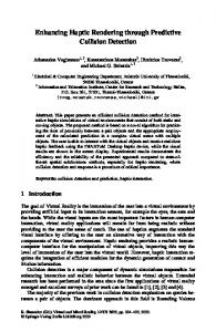
that large number of intersection tests with the same object have to be calculated. In order to reduce the time needed for an intersection test, we have chosen to test the intersection of a grid cell or leaf node with the object's bounding box. One can either chose to use the object's Axis-Aligned Bounding Box (AABB) or the tighter fitting Object-aligned Bounding Box (OBB) [17]. An intersection with an AABB is easier and faster to check. We have, however, chosen to use OBB's. Because of the tighter fit (as can be seen in Fig. 2), an OBB is less likely to have an unnecessary intersection (an intersection with a cell that intersects the bounding box, but not the object). This reduces the number of objects that have to be rendered at run time.

Improving Haptic Rendering of Complex Scenes using Spatial Partitioning

(a) AABB

199

(b) OBB Fig. 2. Comparison of bounding boxes.

In order to minimise the time needed for the intersection tests, we make use of the separating axis theorem [18]. This theorem provides an efficient test for determining if two OBBs overlap (we treat the grid's cells and tree's leaf nodes as OBBs). It states that, if two OBBs do not overlap, an axis exists where the projection of the two OBBs onto the axis do not overlap. This axis is called a separating axis. Furthermore, [18] →

states that only 15 possible axes L have to be checked: →

→

→

L = V xW

→

(1)

→

The vectors V and W in (1) are taken from the OBBs' six box axes. For AABBs, the number of tests in this theorem is reduced to 3. However, the speedup of having a tighter fit in the haptic loop justifies the extra tests in the OBB case.

3

Experiments

Two experiments were conducted in order to assess the usefulness of the algorithms discussed in sections 2.1 and 2.2. Both experiments compared the haptic load of dif-

200

Chris Raymaekers and Karin Coninx

ferent scenes when using different algorithms. A PHANToM 1.0 was used as force feedback device, while the algorithms were implemented using e-Touch beta 3. In the first experiment, objects were placed in a grid of equal sides, as depicted in Fig. 3. These objects were rendered with the standard e-Touch renderer, a grid with 2 x 2 x 2 cells, a grid with 5 x 5 x 5 cells, an octtree with minimum leaf node size of 5mm and maximum 2 objects and an octtree with minimum leaf node size of 5mm and maximum 5 objects. The partitioned space, rendered by the algorithms, was slightly larger than the object grid and, depending on the number of objects, larger than the PHANToM device's workspace.

(a) Experiment 1 (27 objects)

(b) Experiment 2 (20 objects)

Fig. 3. Experimental set-up

For the second experiment, a number of test scenes, containing 10, 20, 50, 100, 200 or 500 randomly placed objects, were prepared (see Fig. 3b). For each number of objects, five different scenes were created. In order to start the test without hindering the PHANToM device, each scene's objects stay out of a small region around the cursor's starting position. This test was conducted with the standard e-Touch renderer, a grid with 2 x 2 x 2 cells, a grid with 5 x 5 x 5 cells, an octtree with minimum leaf node size of 5mm and maximum 2 objects. The objects stayed within a 25cm x 25cm x 25cm large cube. The partitioned space matched this work area.

Improving Haptic Rendering of Complex Scenes using Spatial Partitioning

201

In both experiments, the number of objects were increased for each rendering algorithm until the haptic rendering was no longer stable. The haptic load was assessed using the haptic drivers haptic load tool [6]. Since this is the only way to assess the haptic load, this tool is currently considered a valid (although not precise) means to measure the performance of haptic algorithms. All values that are mentioned in this paper are estimates from the tool's visual output; no exact figures can be given. We determined the maximum haptic load when moving through the virtual world, without touching an object, when statically touching an object and when sliding over an object's surface. In both experiments, the objects were cubes of 5cm x 5cm x 5cm (e-Touch boxes), because they can be efficiently rendered, and thus have little overhead in the rendering process. For this purpose, we extended e-Touch's haptic cube renderer with the separating axis algorithm (see Sect. 2.3). The computer used in the experiments is a dual Pentium III 800 MHz with 128MB RAM, running Windows 2000. Only static scenes were used in these experiments, since dynamic scenes need to be explicitly updated. It is however possible to temporary remove an object from the grid or octtree, use standard rendering during its movement and put it back into the grid or octtree when the movement is finished.

4

Results

4.1

Experiment 1

The first experiment shows that the grid indeed significantly increases the number of objects that can be haptically rendered. When using the standard e-Touch renderer, a grid of 3 x 3 x 3 objects can efficiently be rendered. It is however not possible to stably render a grid containing 64 objects. Table 1 summarises the haptic load for the standard renderer and illustrates the increase of haptic load when touching the object and sliding over its surface. Table 1. Results of experiment 1 for the standard renderer

# objects 8 27 64

No Touch Touch Sliding 35%