especially refer to the deflection of the cantilever: [1] is an example in ... ENSMM - Université de Franche-Comté ..... actions on Automatic Control, AC-26(1), 1981.
Modelling and Robust Position/Force Control of a Piezoelectric Microgripper Micky Rakotondrabe, C´edric Cl´evy and Philippe Lutz Abstract— This paper deals with the control of a piezoelectric microgripper based on two piezocantilevers. To avoid the destruction of the manipulated micro-object and to permit a high accurate positioning, the microgripper is controlled on position and on force. Each piezocantilever is separately modelled and controlled: while the one is controlled on position, the second is controlled on force. Because the models are subjected to uncertainties and the micromanipulation requires good performances, a H∞ robust controller is designed for each system. The experiments end the paper and show that good performances are obtained.
I. Introduction In micromanipulation, i.e. manipulation of object from 1µm to 1mm sizes, the required accuracy is generally sub-micrometric. Instead of hinges, active materials are used to design systems for micromanipulation. In fact, hinges are characterized by frictions and may decrease the performances (accuracy) of the micromanipulation. Among these active materials, piezoelectric materials are widespread because of their fast response time and their high resolution. One of the main applications of piezoelectric materials in microsystems is piezoelectric microgrippers. A piezoelectric microgripper is based on two piezoelectric cantilevers (piezocantilevers). It is used to pick a micro-object, transport and place it with a high positioning accuracy. Nevertheless, to avoid the destruction of the micro-object, a control of the manipulation force is necessary. In the litterature, many studies have been done on the modelling and control of a piezocantilever but few concern a whole microgripper. The majority of these studies especially refer to the deflection of the cantilever: [1] is an example in the linear approach while [2][3][4][5] takes into account the nonlinearities of the material. On the other hand, the control of the force is today a partially solved problematic because it requires the integration of a very small sensor, the use of the piezoelectric properties or a compliant structure. Up to now, very few solutions are proposed: [6][7][8]. In this paper, we propose to model and control a piezoelectric microgripper. In order to ensure good performances for the micromanipulation, a H∞ robust conLaboratoire d’Automatique de Besan¸con LAB CNRS UMR6596 ENSMM - Universit´ e de Franche-Comt´ e 24, rue Alain Savary 25000 Besan¸con - France
{mrakoton,cclevy,plutz}@ens2m.fr
troller is used. The position (directly measured) and the manipulation force (estimated) are considered as the references. The paper is organized as follows. First, the modelling of the microgripper is presented. Then, the design of the H∞ controller for each piezocantilever is presented. Finally, the experimental results are presented and discussed. II. Modelling Let the Fig. 1 present the piezoelectric microgripper manipulating a micro-object. In this figure, Fm is the manipulation force applied by the two piezocantilevers to the micro-object. Our objective is to control the position of the micro-object by means of one piezocantilever and to maintain a constant value of Fm by means of the second piezocantilever. Because the adhesion forces [9] are insignificant relative to the manipulation force range of our concern (more than millinewton), and because we experiment objects from 500µm to 1.5mm in size, they will not be taken into account in this paper. electric connection left piezocantilever
right piezocantilever
Fm
δl Fig. 1.
positive direction (force, deflection)
δr
A piezoelectric microgripper manipulating a micropart.
The relation between the applied voltage Ui , the force Fi applied to the piezocantilever at its tip and the resulting deflection δi , with i ∈ {l, r}, in the static mode is [10]: δi = di · Ui + si · Fi
(1)
where di > 0 is the equivalent piezoelectric constant of the piezocantilever and si > 0 is the equivalent elastic constant. However, it has been shown that the transient part of the (Ui , δi )-transfer and the transient part of the (Fi , δi )transfer of a piezocantilever are similar [11]. Thus, we have:
δi = (di · Ui + si · Fi ) · Di (s)
(2)
where Di (s) (such as Di (0) = 1) represents the dynamic part and s the Laplace variable. On the other hand, the relation between the manipulation force Fm and the contraction of the micro-object is: (δl − δl0 ) − (δr − δr0 ) = so · Do (s) · Fm
(3)
where so > 0 is the elastic constant of the micro-object, Do (s) (such as Di (0) = 1) is its dynamic characteristic and δl0 and δr0 are the deflections of the left and right piezocantilevers before touching the object (Fig. 2).
In both approaches, the models are dependent on the characteristics of the micro-object. In this paper, we choose the second approach because of the simplicity of the models and of the issued controllers. A. Model of the voltage/deflection transfer Here, we model the right piezocantilever. From the second equation of the set (Eq. 4), we have the nominal model: δr = dr · Dr (s) · (Ur + br )
where br = − srd·Fr m is an input disturbance to be rejected. Fig. 3 shows the corresponding scheme.
electric connection left piezocantilever
(5)
br right piezocantilever
Ur Fig. 3.
δl 0 δ r 0 Fig. 2. Initial situation: the micro-object is not in contact with the piezocantilevers.
Noting ∆δ = δl0 − δr0 and replacing Fl = Fr = −Fm in the (Eq. 2), we have: δl = (dl · Ul − sl · Fm ) · Dl (s) δr = (dr · Ur − sr · Fm ) · Dr (s) (4) (δl − δr ) − ∆δ = so · Do (s) · Fm Without loss of generality, we choose the left piezocantilever for the force Fm actuation while the right one for the micro-object position actuation. From the set of equations (Eq. 4), two approaches are possible to model the microgripper: • the first approach uses one bivariable system where the inputs are the two voltages and the outputs are the deflection δr and the force Fm . It takes into account the effects of the piezocantilevers deflections to each other. So, it is possible to design a multivariable controller leading to very good performances. However, this approach needs a precise model, • the second approach consists in modelling independently the two piezocantilevers. While the one is modelled on force, the second is modelled on deflection. The advantage is that the two models are easier than of the first approach. However, since the deflection of one cantilever disturbs that of the other, and vice versa, the design of each feedback controller should takes into account such disturbances.
+
d r ⋅ Dr ( s)
+
δr
Scheme of the nominal model of the right piezocantilever.
B. Model of the voltage/force transfer The left piezocantilever is modelled in this part. From the first and last equations of the set (Eq. 4), we have:
Fm =
1 · Dk (s) · (dl · Dl (s) · Ul − δr − ∆δ) (6) (so + sl )
with: Dk (s) =
(so + sl ) (Do (s) + Dl (s))
(7)
and Dk (0) = 1. The (Eq. 6) clearly shows that the model depends on the characteristics of the micro-object. Nevertheless, it is not practical to identify the model and to synthesize a controller at each change of manipulated micro-object. Thus, we propose to have a nominal model independent of the micro-object characteristics, i.e. so = 0 and Dk (s) = 1, and use a robust controller to ensure the stability and the performances. Such hypothesis will be verified in the experimental results. Finally, we have the following nominal model: Fm =
dl · Dl (s) · Ul + Fpert sl
(8)
where Fpert = − (δr +∆δ) is an output disturbance to sl be rejected. Fig. 4 shows the corresponding scheme.
Fpert
dl ⋅ Dl ( s) sl
Ul Fig. 4.
+
� µm � dr = 0.545 V
Fm
+
(9)
1 1.86×10⁻⁸ ·s2 +4.1×10⁻⁶ ·s+1
Dr (s) =
and
Scheme of the nominal model of the left piezocantilever.
C. Identification For our experiments, we use two unimorph piezocantilevers based on a P IC151 piezolayer [12] and a Copper layer. The sizes of each piezocantilever are: 15mm × 2mm × 0.3mm (length, width and thickness) where the thickness of the piezolayer is 0.2mm . The experimental setup (Fig. 5) is made up of: • the microgripper, • two laser sensors (Keyence sensor with 500nm of accuracy) to measure the deflections of the piezocantilevers, • an amplifier with two lines for Ul and Ur , • a computer-DSpace material to acquire the measurements and to generate the input voltages Ul and Ur .
� µm � dl = 0.525 V
Dl (s) =
(10) 1
1.85×10⁻⁸ ·s2 +2.72×10⁻⁶ ·s+1
Fig. 6 shows the results of (Ui , δi )-transfer function for the right piezocantilever. −70 magnitude [dB] right piezocantilever −80 −90 −100 experimental result
−110 −120 −130
simulation of the model
−140 −150 −160
amplifier piezoelectric microgripper
laser sensor
laser sensor
(a)
microgripper support
right optical sensor
left optical sensor
right piezocantilever
(b)
Fig. 5.
101
102
103 104 pulsation [rad/s]
Magnitude of the right piezocantilever.
Finally, to identify the elastic constant si , a mass is hung on at the tip of each piezocantilever and the resulting deflection � � is measured. We have sr = sl = 1.931 × 10⁻³ m N . Because the characteristics of the micro-object have been neglected in the nominal model, the latter is subjected to uncertainties. Such approach let us avoid the model identification and the controller synthesis of at each change of micro-object. Therefore, we choose a robust controller to ensure the stability and performances robustness face to the uncertainties, we use the H∞ controllers. Moreover, the disturbance rejection will be taken into account during the controller design. III. Control of the deflection δr
15mm left piezocantilever
Fig. 6.
100
Experimental setup.
For each piezocantilever, a harmonic experiment was performed. Afterwards, the (Ui , δi )-transfer function is identified in the frequenty domain. A second order model is assumed to be sufficient for piezocantilevers [13]. We have:
Let the Fig. 7 be the closed-loop scheme. In the figure, δrr indicates the reference input. Two weighting functions are used: W1r for the closed-loop performances and W2r for the disturbance rejection. A. Standard form Let Pr (s) be the augmented system including the nominal system and the weighting functions. Fig. 8 shows the corresponding standard scheme. The standard H∞ problem consists in finding an optimal value γ > 0 and a controller Ki (s) stabilizing the closed-loop scheme of the Fig. 8 and guaranteeing the following inequality [14]:
or
r 2
W
W
εr
δ rr +
Fig. 7.
Kr
-
When the disturbance is a static force, its influence on the has been chosen to be lower than � � µmdeflection . 1.7 10mN
ir
r 1
br
Ur +
Gr = d r ⋅ Dr ( s )
+
δr
1 3·s+1 = 10−3 · r W1 30 × 10−3 · s + 1
The closed-loop scheme with the weighting functions.
δ r er = r ir
From the performances specifications, we choose:
Using the specifications on the disturbance rejection and using the equivalence br = − srd·Fr m , we choose:
or
Pr ( s )
W1r
Ur
εr
K r (s) Fig. 8.
opt γ = 10.1
(11)
where Flow (., .) is the lower Linear Fractionar Transfor(s) mation and is defined here by Flow (Pr (s), Kr (s)) = oerr (s) . From the Fig. 7, we have: or =
· Sr ·
−
W1r
· Sr · Gr ·
W2r
· ir
(12)
−1
where Sr = (1 + Kr · Gr ) is the sensitivity function. Using the condition (Ineq. 11) and the (Eq. 12), we infer: kW1r · Sr k∞ < γ r kW1 · Sr · Gr · W2r k∞ < γ
|Sr | < ⇔
(15)
The computed controller has an order of 5. To minimize the memory and time consumptions in the computer, the controller order has been reduced to 2 using the balanced realization technique [17]. We obtain:
The standard form.
δrr
3·s+1 1 = 0.5 × 10⁻⁷ · r · W2 3 × 10⁻³ · s + 1
C. Calculation of the controller
kFlow (Pi (s), Ki (s))k∞ < γ
W1r
(14)
|Sr · Gr |