Apr 26, 2018 - son log-linear model, extended Hamilton-Grey algorithm. 1 Introduction. The study of ..... an adaptation of the extended Hamilton-Gray (EHG) algorithm described in Chen & Tsay (2011). The ...... 488, John Wiley &. Sons.
Modelling corporate defaults: A Markov-switching Poisson
arXiv:1804.09252v1 [stat.ME] 24 Apr 2018
log-linear autoregressive model Geir D. Berentsen1 , Jan Bulla1, 2 , Antonello Maruotti3 , and B˚ ard Støve1 1
Department of Mathematics, University of Bergen, P.O. Box 7803, 5020 Bergen, Norway Department of Psychiatry and Psychotherapy, University Regensburg, Universit¨atsstraße 84, 93053 Regensburg, Germany 3 Dipartimento di Giurisprudenza, Economia, Politica e Lingue Moderne (GEPLI), Libera Universit`a Maria Ss Assunta, Via Pompeo Magno 22, 00192 Rome, Italy
2
April 26, 2018 Abstract This article extends the autoregressive count time series model class by allowing for a model with regimes, that is, some of the parameters in the model depend on the state of an unobserved Markov chain. We develop a quasi-maximum likelihood estimator by adapting the extended Hamilton-Grey algorithm for the Poisson log-linear autoregressive model, and we perform a simulation study to check the finite sample behaviour of the estimator. The motivation for the model comes from the study of corporate defaults, in particular the study of default clustering. We provide evidence that time series of counts of US monthly corporate defaults consists of two regimes and that the so-called contagion effect, that is current defaults affect the probability of other firms defaulting in the future, is present in one of these regimes, even after controlling for financial and economic covariates. We further find evidence for that the covariate effects are different in each of the two regimes. Our results imply that the notion of contagion in the default count process is time-dependent, and thus more dynamic than previously believed. Keywords: Markov-switching model, corporate defaults, MS-PLLAR, integer valued time series, Poisson log-linear model, extended Hamilton-Grey algorithm.
1
Introduction
The study of modeling and forecasting corporate defaults has been intensified in the recent years. A major drive for this increased interest has been the need to find an explanation for the clustering of defaults observed. In essence, two explanations have been proposed for this stylized fact. First, each
1
firm can be considered exposed to a ”systematic risk”, represented by common economical and financial factors. Second, one firm’s default may increase the likelihood of other firms defaulting, resulting in so-called ”contagion effects”. Both explanations are plausible approaches describing a clustering of the observed defaults, and may occur separately but also jointly. From a practical perspective, one core issue has been to distinguish between these two explanations. In particular, revelation of the presence of a contagion effect is important: disregarding this effect may lead to an underestimation of probabilities of defaults (PD), because most credit models in practice assume that default events are conditionally independent (i.e. given observable common factors, defaults are independent in time). Consequently, ignoring possible dependence structures in corporate defaults may cause that the amount of capital held by banks and other financial institutions exposed to credit portfolios is insufficient. Several studies have examined the default clustering fact in the past, and following Agosto et al. (2016), one can broadly divide the studies into two categories. In the first category, firm-level data are available in addition to macroeconomic variables and default times for firms are recorded. Then, the default times are usually modeled by Poisson processes with both types of covariates entering the default intensities. Studies in this category are e.g. Das et al. (2007), who provide evidence that the ”systemic risk” on its own cannot explain the degree of clustering observed in U.S. industrial defaults, and Lando & Nielsen (2010), who does not report a contagion effect using another type of test procedure. The second category uses aggregate data, where the number of defaults in a given time period is collected together with macroeconomic variables. Several papers have used this approach, e.g. Koopman et al. (2012), who use a high-dimensional and partly nonlinear, non-Gaussian dynamic factor model for counts of default, where the probability of default is time-varying and a function of macroeconomic covariates. However, their model specification requires computationally demanding Monte Carlo methods. They find that the extreme tail clustering in defaults cannot be captured using macro variables alone. Another study in the second category was performed by Azizpour et al. (2017). They find strong evidence that contagion is a main source for the clustering behavior. The papers most related to our approach are Agosto et al. (2016) and Sant’Anna (2017), both of which belong to the second category as well. Agosto et al. (2016) introduce a class of Poisson autoregressive models with exogenous covariates to model the count of defaults. They find evidence of a contagion effect, which diminishes in recent years. Sant’Anna (2017) introduces new test procedures permitting to carry out model checks for dynamic count models, and finds evidence of a contagion effect as well. In this paper we propose an extension to the count time series model class. We allow for a model that can characterize the time series behaviors in different regimes. By permitting switching between these regime, such a model is able to capture more complex dynamic patterns. In essence, we have a model where (some of) the parameters depend on the state of an unobserved Markov chain. There has been some work in this direction, confer e.g. Kirch & Kamgaing (2016b). This also means that the macroeconomic and financial variables can have different effects on the default intensity depending on the regime. This extension is inspired by some of the results in Agosto et al. (2016), in where they show that there are structural instabilities in the model parameters over the sample period. We should be able to pick up such effects by permitting for several regimes. We further will be able to provide more evidence for or against the contagion effect.
2
In the past years models for count time series have been intensively studied, in particular due to the wide area of applications. This paper contributes to the literature on autoregressive models for count time series subject to structural changes. Time series often experiences a structural change, and the problem of change point detection has been a central issue in the literature: see e.g. Kirch & Kamgaing (2016a) for a recent review. The change point test for univariate integer-valued time series has been studied by many authors, see e.g. Kang & Lee (2009), Franke et al. (2012), Fokianos et al. (2014), Kang & Lee (2014), Doukhan & Kengne (2015) and Diop & Kengne (2017), while a procedure on testing for bivariate models is given in Lee et al. (2016). A natural extension will be to allow for a count time series model with regimes, and to the best of our knowledge, this is the first paper employing such an idea in the setting of autoregressive count time series. The paper is organized as follows. In Section 2, we extend the Poisson log-linear autoregressive count time series model allowing for regime-switching, and interpret it in the context of modeling defaults. In Section 3 we present the algorithm for how the model can be estimated, and adress both inference about the underlying regimes and prediction. In Section 4 we provide a simulation study for assessing the performance of the algorithm, and perform the empirical analysis of the counts of corporate defaults. Finally, Section 5 provides some concluding remarks.
2
The Markov-switching Poisson log-linear autoregressive
model In this section we define the Markov-switching Poisson log-linear autoregressive (MS-PLLAR) model and interpret it in the context of modeling defaults.
2.1
Definition
Let {Yt } be a count time series such as corporate defaults, and let {Xt } denote a r-dimensional timevarying exogenous covariate vector, i.e. Xt = (Xt,1 , . . . , Xt,r )t . To capture possible regime changes in {Yt } we introduce an unobserved first-order Markov process {St } taking discrete values 1, . . . , m. Let Γ = {γij } denote the m × m transition probability matrix of {St }, where the terms {γij } represent the probability of moving from the ith state at time t−1 to state j at time t, where h, k = 1, . . . , m. We assume that St is time-homogeneous and stationary, with δ = (δ1 , . . . , δm ) denoting the stationary distribution. Furthermore, Y (t) represents the vector of observations (Y1 , . . . , Yt )t , and the vector of hidden states S (t) is defined analogously. Similarly, X (t) denotes the matrix of covariates (X1 , . . . , Xt )t and βSt denotes the vector of corresponding state-specific effects (β1,St , . . . , βr,St )t . For modeling corporate defaults we consider a MS extension of the Poisson log-linear autoregressive model studied in Fokianos & Tjøstheim (2011) defined by Yt | Ft−1 ∼ Poisson(λt ),
ηt = log(λt ) = dSt + aSt ηt−1 + bSt log(Yt−1 + 1) + βS0 t Xt ,
t≥1
(2.1)
with information set Ft = {Y (t) , X (t+1) , S (t+1) , θ} and θ denoting the vector of parameters in the model, i.e. θ =
�
m {ak , bk , dk , β1,k , . . . , βr,k }m k=1 , {γij }i,j=1 . Since
3m + rm + m(m − 1) free parameters.
3
Pm j=1
γij = 1, the model contains
2.2
Interpretation of the model
For m = 1 (2.1) reduces to the log-linear autoregressive model of Fokianos & Tjøstheim (2011). That is, the linear predictor ηt reduces to ηt = log(λt ) = d + aηt−1 + b log(Yt−1 + 1) + β 0 Xt .
(2.2)
Note that in this framework, we can allow for β 0 Xt < 0. The roles of the terms of (2.2) can be interpreted as follows. First, the parameter d simply fixes the overall intensity level. Then, changes in the systematic risk are best captured by the term β 0 Xt , which models the impact of exogenous variables representing macroeconomic or financial risks on the (log-)intensity. Moreover, assuming b > 0, the second-last term of (2.2), b log(Yt−1 ), may indicate the presence of contagion effects since increases in Yt−1 lead to an intensity increase. The term aηt−1 is slightly less straightforward to interpret. On the one hand, it may either have an amplifying effect on high intensity values (for a > 0), or dampen extreme values (for a < 0). On the other hand, aηt−1 also implicitly models a dependence of the intensity on all previous lags of both Yt and exogenous variables Xt . This is best illustrated by assuming for simplicity that Y0 and η0 are known quantities. Assuming a 6= 1, we then obtain ηt = d
t−1
t−1
i=0
i=0
X i 0 X i 1 − at a β Xt−i a log(1 + Yt−i−1 ) + + at η0 + b 1−a
(2.3)
by repeated substitution of (2.2). From Equation (2.3) we see that all terms related to systematic risk propagate to future values of the (log-)intensity as
Pt−1 i=0
ai β 0 Xt−i , which we can therefore interpret as
a term representing the overall macroeconomic or financial risk. Similarly, the terms linked to contagion effects sum up to b
Pt−1 i=0
ai log(1 + Yt−i−1 ), and thus propagate to future values of the (log-)intensity as
overall feedback-effect, i.e. the overall contagion. Summarizing, the inclusion of the term aηt−1 in (2.2) represents a parsimonious way for allowing the intensity to depend on all previous lags of both Yt and exogenous variables Xt . For the MS case, i.e. m ≥ 2, the interpretation of the last three terms of (2.1) are similar to the simple case. However, the model coefficients are driven by the unobserved Markov chain, which permits more flexibility since it allows the above described effects to vary in time. For example, exogenous variables may have a significant impact on the intensity in one state, while these effects remain negligible in another state. Moreover, the first parameter of (2.2) becomes dSt and permits to model changes in the systematic risk, resulting e.g. from unobserved covariates. To summarize; we thus follow Agosto et al. (2016) for allowing for differentiation between systematic risk and contagion, and we note that in the case where b = 0 in equation (2.2), the model imply conditional independence between current and past defaults. Similarly, in the MS case, we will examine the estimated parameters of bSt for all regimes. Thus, we may actually observe that in some regimes we may have contagion, and in others not. We thus allow for a more dynamic process of the corporate default counts, but retain an analogous interpretability as the PARX model of Agosto et al. (2016).
4
3
Estimation and inference
In this section we present the algorithm for estimating the model parameters, address inference about the underlying regimes, and derive a couple of prediction techniques.
3.1
The regime path dependence problem
The computation of ηt in (2.1) requires the comprehensive information set Ft−1 = {Y (t−1) , X (t) , S (t) , θ} due to its dependence on past values of ηt . In particular, ηt depends on the complete regime path S (t) , which causes difficulties within the estimation procedure. The likelihood, denoted by L(θ) of the observations {Y (T ) }, is given by m X
L(θ) = P (Y (T ) = y (T ) | θ) =
P (Y (T ) = y (T ) | S (T ) = s(T ) )P (S (T ) = s(T ) )
s1 ,...,sT =1 m
=
X s1 ,...,sT =1
T
Y exp(−λt )λyt t
t=1
yt !
P (S1 )
T Y
(3.1)
! P (St = st | St−1 = st−1 )
.
t=2
A direct computation of (3.1) is problematic since λt = exp(ηt ) has to be derived recursively by (2.1) for each of the mT different regime paths. As a consequence, direct computation of (3.1) quickly becomes infeasible with increasing T . This problem is often termed the path-dependence problems for Markovswitching (MS) models, and was first pointed out by Hamilton & Susmel (1994) when discussing the possibility of a MS generalized autoregressive conditional heteroskedasticity (MS-GARCH) model. The problem for the MS-GARCH model was later adressed in the work of Gray (1996), see also Augustyniak (2014) and references therein. In the seminal work of Hamilton (1989) a much used algorithm for estimating MS autoregressive (MS-AR) models is proposed. However, for MS autoregressive moving-average (MS-ARMA) models path-dependence problems arise due to the moving-average component (see e.g. Billio & Monfort 1998), in which case the algorithm of Hamilton fails. Analogously, with the exception of the case a = 0 in (2.1), a direct adaptation of the Hamilton algorithm to the MS-PLLAR model faces path-dependence type problems. Such difficulties are the very ones addressed by the principles presented in Gray (1996), which build the foundation for our approach. More precisely, in this paper we approximate (3.1) using an adaptation of the extended Hamilton-Gray (EHG) algorithm described in Chen & Tsay (2011). The EHG algorithm avoids the path dependence problem by combining the algorithm of Hamilton (1989) and the ideas of Gray (1996) of recursively replacing certain quantities, in our case ηt , with its expectation. This permits to trace only the m2 possible regime paths from time t − 1 to time t instead of the full path, and then to iteratively replace ηt with the corresponding conditional expectations that are consistent with these paths. Hence, the estimation routine falls into the framework of Hamilton (1989). In order to separate our adaption from the original EHG algorithm tailored for MS-ARMA models, we refer to the adaptation as the MS-PLLAR EHG (or only EHG in short) algorithm.
5
3.2
The MS-PLLAR EHG algorithm
For tracing the regime path from time t−1 to time t, we create a new state variable St∗ = 1, 2, . . . , m2 . This variable is defined such that each state of St∗ represent a particular regime path (St−1 = st−1 , St = st ), i.e.
St∗ =
1 2
Note that
St = 1,
if
St = 2,
.. .
St∗
if
St−1 = 1 St−1 = 1 (3.2)
.. .
m2
St = m,
if
St−1 = m
also inherits the Markov property from St . The dynamics of St∗ can be characterized via a
∗ first-order Markov chain with a m2 × m2 transition probability matrix Γ∗ = {γkh } that can be derived
from Γ. For example, for m = 2 one obtains
∗ γ11
∗ γ12
∗ γ13
∗ γ14
∗ γ21 Γ∗ = ∗ γ31
∗ γ22
∗ γ23
∗ γ32
∗ γ33
∗ γ24
∗ γ42
∗ γ43
∗ γ41
γ11
0 = ∗ γ34 γ11 ∗ γ44
0
γ12
0
0
γ21
γ12
0
0
γ21
0
γ22
. 0
γ22
The new state variable St∗ is crucial for determining the aforementioned conditional expectations of ηt . For each time t, the conditional expectations will be collected in a vector denoted by Λt . The computation of Λt bases on a specific information set denoted by Ωt−1 as well as Λt−1 , which are given by Ωt−1 Λt−1
= =
{Y (t−1) , X (t) , Λt−1 , θ},
�
�
∗ ∗ ηˆt−1|St−1 ˆt−1|St−1 ˆt−1|S ∗ =1,Ωt−2 , η =2,Ωt−2 , . . . , η
=m2 ,Ωt−2 t−1
.
(3.3)
∗ Thus, the vector Λt−1 contains the corresponding expectations of ηt−1 conditional on St−1 = j, j =
1, . . . , m2 and the information set Ωt−2 , indicating the recursive structure of the algorithm. The first step in deriving Λt is to compute the expectations of the elements in Λt−1 conditional on St∗ = j, j = 1, . . . , m2 and the information set Ωt−1 by ∗ ∗ ηˆt−1|St∗ =j,Ωt−1 = E(ˆ ηt−1|St−1 ,Ωt−2 | St = j, Ωt−1 ) 2
=
m X
∗ ∗ = i | St∗ = j, Ωt−1 )ˆ ηt−1|St−1 P (St−1 =i,Ωt−2
i=1 2
=
m X i=1
∗ ∗ γij P (St−1
∗ = i | Ωt−1 )ˆ ηt−1|St−1 =i,Ωt−2
P (St∗ = j | Ωt−1 )
(3.4)
,
∗ ∗ ∗ where j = 1, . . . , m2 . The substitution of P (St∗ = j | St−1 = i, Ωt−1 ) with P (St∗ = j | St−1 = i) = γij is
valid due to the Markov property of St∗ . This step can be seen as a Bayesian update of the elements of Λt−1 with the information set Ωt−1 . For the next step, let St (St∗ = j) be the value of St given that St∗ is in state j. Since each state of St∗ represent a particular realization of (St−1 , St ), the elements of Λt can be computed by forwarding ηˆt−1|St∗ =j,Ωt−1 consistently with the regime path corresponding to St∗ = j,
6
j = 1, . . . , m2 : ηˆt|St∗ =j,Ωt−1 = E(ηt | St∗ = j, Ωt−1 ) = dSt (St∗ =j) + aSt (St∗ =j) ηˆt−1|St∗ =j,Ωt−1 + bSt (St∗ =j) Yt−1 + βSt t (St∗ =j) Xt ,
j = 1, . . . , m2 (3.5)
Hence, it is possible to compute Λt by means of the equations (3.4)-(3.5), provided that of the quantities ∗ P (St−1 = j | Ωt−1 ) and P (St∗ = i | Ωt−1 ), i, j = 1, . . . , m2 occurring in (3.4) are known. One may note
that these two quantities are already a by-product of the previous iteration step (carried out for t − 1) through the filter defined by the equations (3.6) - (3.9) below. In detail, under the Poisson assumption the probability of Yt = yt conditional on St∗ and Ωt−1 is P (Yt = yt |
St∗
= j, Ωt−1 ) =
ˆ t|S ∗ =j,Ω λ t−1 t
�y t
ˆ t|S ∗ =j,Ω exp −λ t−1 t
�
yt !
,
(3.6)
ˆ t|S ∗ =j,Ω where λ = exp(ˆ ηt|St∗ =j,Ωt−1 ). By summing over all states, the probability of Yt = yt conditional t−1 t on Ωt−1 then becomes 2
P (Yt = yt | Ωt−1 ) =
m X
P (Yt = yt | St∗ = i, Ωt−1 )P (St∗ = i | Ωt−1 ),
(3.7)
i=1
which effectively corresponds to a discrete mixture of Poisson-distributed variables. Subsequently, the so-called filtering probabilities can be computed by P (St∗ = j | Ωt ) =
P (St∗ = j | Ωt−1 )P (Yt = yt | St∗ = j, Ωt−1 ) P (Yt = yt | Ωt−1 )
(3.8)
for j = 1, . . . , m2 , and the one-step ahead predictive probabilities trough 2
∗ P (St+1 = j | Ωt ) =
m X
∗ P (St+1 = j | St∗ = i, Ωt )P (St∗ = i | Ωt )
i=1
(3.9)
2
=
m X
∗ γij P (St∗
= i | Ωt )
i=1
for j = 1, . . . , m2 , where the last equality is a direct consequence of the Markov property of {St∗ }. Last, by recursively computing equations (3.4)-(3.9) we can obtain the quasi-log-likelihood log L∗ (θ) =
T X
log P (Yt = yt |Ωt−1 ),
(3.10)
t=1
where P (Yt = yt |Ωt−1 ) is given by (3.7). Figure 1 displays an overview of the evolution of Λt for m = 2. Intuitively, the two equations (3.8) and (3.9) serve as adaptive inference tool for St∗ . On the one hand, the one-step ahead probability P (St∗ | Ωt−1 ) obtained by Equation (3.9) at time t − 1 act like a ”prior” distribution of St∗ given Ωt−1 . On the other hand, this quantity is then corrected at time t by the actual value of Yt through Equation (3.8), resulting in the ”posterior” distribution of St∗ given Ωt , P (St∗ = j | Ωt ).
7
Both equations also play an important role for the inference for St∗ , which translates to inference about the actual state St at time t. This is subject of the following Section 3.3. Last, the algorithm being recursive, it needs to be initialized. This part, carried out at t = 1, can be completed by initializing only the equations (3.5) - (3.9), provided that we possess starting values for Y0 , Λ0 and P (S1∗ = j | Ω0 ), j = 1, . . . , m2 . Starting values for Y0 and Λ0 and alternative initialization methods are discussed in detail in Appendix A.1. Moreover, for both initializing the algorithm and throughout the optimization procedure we assume (P (S1∗ = 1 | Ω0 ), . . . , P (S1∗ = m2 | Ω0 )) = δ ∗ , where δ ∗ is the stationary distribution of St∗ . Appendix A.1 illustrates this part as well.
3.3
Inference about the states
Given the information set Ωτ with τ = {1, . . . , T }, inference about the state St at any time t may be carried out via probabilities of the form P (St = j | Ωτ ), j = 1, . . . , m. Given analogous probabilities for the process St∗ defined by (3.2), P (St = j | Ωτ ) can be computed by 2
P (St = j | Ωτ ) =
m X
2
P (St =
j, St∗
= i | Ωτ ) =
i=1
where
m X
P (St∗ = i | Ωτ )1 [St (St∗ = i) = j] ,
(3.11)
i=1
1 [·] corresponds to the indicator function. Thus, the filter probabilities P (St = j | Ωt ) and one-
step ahead probabilities P (St+1 = j | Ωt ), j = 1, . . . , m, can be computed directly by (3.11) once the corresponding probabilities for the process St∗ have been obtained through the equations (3.8) and (3.9), respectively. Furthermore, the smoothing probabilities P (St | ΩT ), j = 1, . . . , m, can be derived. These represent the inference about St given the information set ΩT , and are of particular interest when analyzing data in in-sample settings. Similar to the filter and one-step ahead probabilities, the smoothing probabilities can be computed by (3.11), provided that the corresponding smoothing probabilities for St∗ are available. For this purpose, we follow the approach of Kim (1994). First, by the Markov property of St∗ we have that ∗ ∗ P (St∗ = i | St+1 = j, ΩT ) = P (St∗ = i | St+1 = j, Ωt ) =
∗ P (St∗ = i | Ωt ) γij , ∗ P (St+1 = j | Ωt )
Secondly, the smoothing probabilities for St∗ can be represented as 2
P (St∗ = i | ΩT ) =
m X
∗ ∗ P (St+1 = j | ΩT )P (St∗ = i | St+1 = j, ΩT )
j=1
(3.12)
2
=
P (St∗
= i | Ωt )
m ∗ ∗ X γij P (St+1 = j | ΩT ) j=1
∗ P (St+1 = j | Ωt )
for i, j = 1, . . . m2 . Thirdly, using the quantities obtained from Equation (3.8) and (3.9) as well as the filter (smoothing) probabilities P (ST∗ = j | ΩT ), j = 1, . . . , m2 as initial values, we are able to iterate backwards through Equation (3.12). Hence, this recursive procedure permits to calculate the smoothing probabilities for St , t = T − 1, . . . , 1 via Equation (3.11). Estimates of the filter, one-step ahead, and smoothing probabilities result from replacing θ with the quasi
8
maximum-likelihood estimate (QMLE) θˆ in Ωτ , where τ = t − 1, t and T . Figure 2 provides an example for the estimated smoothing probabilities illustrated by means of a simulated time series.
3.4
Prediction and model assessment
A natural one-step ahead prediction YˆT +1 for YT +1 is given by the expectation of YT +1 conditional on the information set ΩT , which includes information on potential covariate at time T + 1 by definition. ˆ T +1|Ω follows Consistent with the Poisson assumption, denoting YˆT +1 = λ T
2
ˆ T +1|Ω = E(yT +1 | ΩT ) = λ T
m X
E (yT +1 | ST∗ +1 = i, ΩT ) P (ST∗ +1 = i | ΩT )
i=1
(3.13)
2
=
m X
ˆ T +1|S ∗ =i,Ω P (ST∗ +1 = i | ΩT ), λ T T +1
i=1
ˆ T +1|S ∗ =i,Ω = exp(ˆ ηT +1|ST∗ +1 =i,ΩT ) , i = 1, . . . , m2 are available where P (ST∗ +1 = i | ΩT ) and λ T T +1 from the T th and T + 1th recursion of the MS-PLLAR EHG algorithm, respectively. Provided that we ˆ T +k|Ω for YT +k can also be possess covariate information up to time T + k, k-step ahead predictions λ T
obtained. For achieving this, the MS-PLLAR EHG algorithm needs to be executed up to time T + k while iteratively replacing the unobserved observations YT +1 , . . . , YT +k−1 in ΩT +1 , . . . , ΩT +k−1 by their ˆ T +1|Ω , . . . , λ ˆ T +k−1|Ω . In practice, θ is replaced by the QMLE respective one-step ahead predictions λ T T ˆ θ based on y1 , . . . , yT in ΩT +1 , . . . , ΩT +k−1 . Similarly, in case covariates are not observed beyond T + 1, these also need to be replaced by some type of predicted values. In a post-processing situation where y1 , . . . , yT have been observed, predictions of y1 , . . . , yT also provide valuable information about the model fit since they serve for computing residuals. Analogously to (3.13), one-step ahead predictions for t = 1, . . . , T are given by 2
ˆ t|Ω λ = E(yt | Ωt−1 ) = t−1
m X
E (yt | St∗ = i, Ωt−1 ) P (St∗ = i | Ωt−1 )
i=1
(3.14)
2
=
m X
ˆ t|S ∗ =i,Ω P (St∗ λ t−1 t
= i | Ωt−1 ),
i=1
ˆ t|S ∗ =i,Ω where P (St∗ = i | Ωt−1 ) and λ = exp(ˆ ηt|St∗ =i,Ωt−1 ), i = 1, . . . , m2 are available from the t−1 t t − 1th and tth recursion of the MS-PLLAR EHG algorithm, respectively. However, this prediction can be improved by utilizing the smoothing probabilities, which are available in a post-processing situation, thus
2
ˆ t|Ω = λ T
m X
ˆ t|S ∗ =i,Ω P (St∗ = i | ΩT ), λ t−1 t
(3.15)
i=1
ˆ t|Ω is somewhat lax since λ ˆ t|Ω 6= E(Yt | ΩT ). Figure 2 displays this prediction where the notation λ T T method for a simulated time series. An alternative approach is to recursively compute ηt in (2.1) along the regime-path deemed most likely by the smoothing probabilities and take exp(ηt ) as an in-sample predictor of Yt . However, this will be a poor prediction if the states are not well separated, or if smooth
9
transition periods between regimes occur in the data. Hence, in general weighted averages such as (3.14) and (3.15) are preferred, and we will use (3.15) in what follows. Note that the plug-in value of θ in the MS-PLLAR EHG algorithm is the only difference between in-sample and out-of-sample predictions. Given predictions of y1 , . . . , yT , we can compute the Pearson residuals by ˆ t|Ω )/ rt = (yt − λ T
q
ˆ t|Ω λ T
(3.16)
for t = 1, . . . , T . Under the correct model, the sequence rt should resemble white noise with constant variance. The empirical autocorrelation function (ACF) of these residuals can be inspected to check for the presence of serial dependence which is not captured by the model. Following (Kedem & Fokianos 2005, section 1.6 and 1.8), the mean square error (MSE) of the Pearson residuals given by
PT t=1
rt2 /(T − p),
where p denotes the number of parameters in the model, serves for evaluating competing models. Last, ˆ t|Ω against the squared raw the Poisson assumption can be inspected by plotting the predictions λ T ˆ t|Ω )2 . In this plot, points scattering symmetrically around the line y = x indicated a residuals (yt − λ T
good model fit.
4
Simulation and empirical analysis
In this section we present results of a simulation study and an empirical analysis corporate defaults.
4.1
Simulation study
In the following, we report the results from a simulation study designed for assessing the finite sample performance of the QMLE’s derived in Section 3.2. The study bases on 1000 simulated time series of length T = 200, 500, 1000, respectively, from two-state MS-PLLAR models subject to different parametrizations. These are termed Case 1 and Case 2, Table 1 summarizes the different parameter values: in Case 1 the two regimes are well separated in terms of both dependence structure (parameter a and b, respectively) and level (d parameter, relative to a and b). The parameters of the first regime are taken from the simulation study conducted in Fokianos & Tjøstheim (2011), and produce a time series with negative correlations at lag one. On the contrary, time series with strong positive correlation for several lags are characteristic for the second regime. Moreover, averaging the time series value in regime one for very long simulated time series results in the value 1.30, compared to 15.64 in regime two. For Case 2, the differences between regimes are more subtle. Both regimes produces positive correlations for several lags, but with stronger lag correlations in the second than in the first regime. The long run average in state one equals 8.24, compared to 15.64 in state two. Therefore, compared to Case 2 one can expect higher precision of the estimates in Case 1. Figure 2 displays a simulated time series for Case 2. The true parameter values of each case served for initializing the estimation procedure. Table 2 summarizes the results of the simulation study. The bias values correspond to the average estimated value of all runs minus the corresponding true parameter value. Similarly, the standard error (SE) is defined as the sample standard deviations of the estimates obtain by simulation. We also ˆ described in Appendix A, which is based on the investigate the adequacy of the standard error se(θ)
10
delta-method and the exact Hessian. For this purpose, the reports the average estimated standard error of all runs (Sc E) as well, which can be compared in turn with the sample standard deviation (SE). With the exception of Case 2 with n = 200, the bias is low. In both Case 1 and Case 2 the SE decreases as n increases, but as expected there is more uncertainty related to the parameters in the second case. In particular for n = 200, the standard error (Sc E) seems to be slightly underestimating compared to the sample standard deviations (SE), which is not atypical for models of such complexity. However, for n = 500, 1000 SE and Sc E are approach each other. Figure 3 and 4 display the relative frequency of the ˆ obtained from each run compared to the standard normal density standardized quantities (θˆ − θ0 )/se(θ) for the two cases. Apart from the parameters of the Markov chain, which lie close to the border of the set of possible values, all other parameters show not stronger deviations from normality.
4.2
Empirical analysis
In this section we provide an analysis of corporate default counts in the US, using the MS-PLLAR model introduced in Section 2. The US defaults count data corresponds to the monthly number of bankruptcies filed in the United States Bankruptcy courts, and is available from the UCLA-LopPucki Bankruptcy Research database (see http://lopucki.law.ucla.edu). These data cover the period from January 1985 to September 2017, in total 393 monthly observations. It consists of the counts of defaults of all large, public companies, where large is defined as having declared more than US$ 100 million in assets the year before the firm filed the bankruptcy case, measured in 1980 dollars. A company is considered public if it had reported to the Securities and Exchange Commission (SEC) in the last three years prior to the bankruptcy. The count of monthly bankruptcies are aggregated by the calender month in which the bankruptcy was filed. Over the sample period a total of 1065 defaults is counted, Figure 5 displays the time series together with recession periods. The recession periods used, are the NBER based recession indicators for the United States (USREC) available from the St. Louis Fed online database FRED. Figure 6 shows a plot of the autocorrelation function of the observations. As highlighted by other studies, these two figures illustate some stylized facts: first, the existence of default clusters; second, the high temporal dependence in the count of defaults; third, overdispersion of the distribution of default counts, as the empirical average is 2.42 while the empirical variance is 6.50. Even though the default counts are available since October 1979, we only use data from 1985 onward to avoid some extreme structural breaks in the covariates, cfr. Sant’Anna (2017). These data have already been studied by several other authors (e.g. Sant’Anna 2017), covering a slightly shorter time span. Furthermore, other studies (e.g. Agosto et al. 2016, Azizpour et al. 2017) base on data exhibiting comparable dynamic patterns from Moody’s Default Risk Service. The purpose of the study is to examine whether the common systematic risk variables can explain the default clustering observed, or if there is default clustering beyond this, i.e. due to the presence of a contagion effect. In addition, as we fit Markov-switching models, we are able to examine whether the effect of the covariates are time-heterogeneous or not. Finally, we are able to reveal if the contagion effect is present in all regimes or not.
11
4.3
Excluding exogenous covariates
We start the empirical analysis by excluding covariates, and focus on determining the number of regimes present for the corporate default series. That is, we fit model (2.1) excluding the term β 0 Xt , and set m equal to 1, 2, and 3 regimes. Table 3 reports a comparison between the different models, while Table 4 shows the estimated parameters for the three models. The MSE marginally favors the model with three regimes, however both the AIC and BIC rank the model with two regimes above the model with m = 3. The one-state model is ranked last, except when using the BIC. Hence, the two-state model represents a suitable choice overall. We further note that the parameter estimates for the model with one regime correspond relatively well to those obtained for the second state in the model with m = 2 (i.e. a2 , b2 and d2 are comparable to a, b and d). The positive sign of the estimated b parameter indicates that the previously observed number of defaults increases the intensity in the current month. However, we cannot reject that d = 0, a = 1, b = 0 for the first state in the two-state model. Consequently, solving η = d + aη + b log(yt−1 + 1) for η results in η = η, indicating a constant intensity. In other words, this model can be characterized by one regime with close to constant default intensity one the one hand, and a second state subjet to more dynamics on the other hand. The model with three regimes resemble the model with two regimes, but with an additional ”medium” dynamic state, as seen from the parameter estimates. Figures 7, 8, and 9 show predictions from the fitted models, and the smoothing probabilities for the model with m equal to two and three, respectively. Based on this analysis and the model comparison, we remain with our previous conclusion that two-regime model is a suitable approach for extending our analysis by including covariates in the intensity equation.
4.4
Including exogeneous covariates
We will use a number of macroeconomic and financial variables that represent the common systematic risk corporations face as explanatory variables. Similar to Sant’Anna (2017), we use monthly variables collected from the St. Louis Fed online database FRED. The variables considered are the industrial production index (INDPRO), new housing permits (PERMIT), civilian unemployment rate (UNRATE), Moody’s seasoned baa corporate bond yield (BAA), 10-years treasury constant maturity rate (GS10), federal funds rate (FEDFUNDS), producer price index by commodity for final demand: finished goods (PPIFGS), and produce price index: fuels and related energy (PPIENG). In addition, we collected the variables S&P500 annualized returns (SP500ret) and S&P500 annualized return volatility (SP500vol) from DataStream. The variables INDPRO, PERMIT, PPIFGS and PPIENG are expressed as yearly growth rates, whereas the variables UNRATE, BAA, FEDFUNDS, GS10, SP500ret and SP500vol are expressed as yearly differences. Most of these covariates have been found to have significant impact on default rates and were used in similar studies (see, e.g., Das et al. 2007, Duffie et al. 2009, Giesecke et al. 2011, Agosto et al. 2016, Azizpour et al. 2017). As described in the section above, we apply model (2.1) with two regimes, and fit separate models
12
using only one covariate for each. This results in ten fitted models, Table 5 reports a model comparison. In the same table, we also report whether the covariate included in each model is found significant or not in any of the two regimes. A clear pattern occurring is that none of the covariates is significant in both regimes, and most are only significant in the most dynamic regime (i.e. number two). In particular, the covariates related to the financial market (SP500ret, SP500vol) are significant in the second regime, which is in line with findings of Agosto et al. (2016). Figure 10 displays the temporal trajectories of the covariate effects obtained from ˆ = βˆ1 P (St = 1 | ΩT ) + βˆ2 P (St = 2 | ΩT ) β(t) These trajectories indicate the temporal variation of covariate effects on the number of defaults. As noted in Section 2.2, the parameter b should be equal to zero in the case of conditional independence. From the estimates of this parameter, we test the null hypothesis H0 : bm = 0 (for m = 1 and 2, i.e. in both regimes separately). The results show that this hypothesis is rejected for all models for the second regime, but cannot be rejected for all models for the first regime. This implies the presence of contagion in the second regime, but not in the first, thus the notion of contagion is indeed time-varying. These findings are in line with Agosto et al. (2016), where systematic risk factors have been able to explain the default clustering observed in the recent years by a more ad-hoc approach of fitting models to sampling periods lying in different time windows.
5
Concluding remarks and outlook
In this paper, we have introduced the Markov-switching Poisson log-linear autoregressive (MS-PLLAR) model, and developed a QMLE using an adaptation of the extended Hamilton-Grey (EHG) algorithm to avoid path-dependence problems. A simulation study indicates that the proposed QMLE is well-behaved. The MS-PLLAR model is suitable to model count time series of corporate defaults, as they are correlated over time and exhibit the default clustering effect, i.e. high peaks in clusters. By using the MS-PLLAR model, we provide evidence that the time series of counts of US default consist of two regimes and that the contagion effect, i.e. that past defaults impact the probability that firms default in the future, is present in one of these regimes. We also note that the coefficients of the covariates are different in each of the regimes. In conclusion, the notion of contagion in the default process is slightly more delicate than previously believed. In the paper, we have only fitted models with one covariate. Thus, the natural next step in the empirical analysis is to include the most significant covariates successively in the model, and then perform the the test for contagion as above. We leave this for future research. Moreover, several alternative model specifications come to mind as potential research subjects as well. For example, the inclusion of further lags for covariates and response or different link functions. In addition, other choices of conditional distribution Yt | Ft−1 are possible. For example, one can assume Yt | Ft−1 ∼ N egBin(λt,k , φk ) where (see Christou & Fokianos 2014) the negative binomial distribution is parameterized in terms of its (state-
13
dependent) mean λt and a (state-dependent) dispersion parameter φSt : P (Yt = y | Ft−1 ) =
Γ(φSt + y) Γ(y + 1)Γ(φSt )
�
φSt φSt + λt
�φSt �
λt φSt + λt
�y (5.1)
It follows that Var(Yt = y | Ft−1 ) = λSt + λ2t /φSt in contrast to the Poisson case where Var(Yt = y | Ft−1 ) = E(Yt = y | Ft−1 ) = λt . The mean parameter λt can be modeled both with a linear and loglinear conditional mean. Such an extension should not pose major obstacles, since, on the one hand, the estimation procedure described in Section 3 is not confined to the Poisson distribution nor the log-linear specification of the conditional mean given in (2.1). On the other hand, however, some modifications are needed to accommodate regression on past values ηt−l and Yt−l for t > 1. These modifications entails tracing the state-paths over more lags and expanding the information set (3.3) analogously to the procedure described in Chen & Tsay (2011).
14
References Agosto, A., Cavaliere, G., Kristensen, D. & Rahbek, A. (2016), ‘Modeling corporate defaults: Poisson autoregressions with exogenous covariates (parx)’, Journal of Empirical Finance 38, 640–663. Augustyniak, M. (2014), ‘Maximum likelihood estimation of the markov-switching garch model’, Computational Statistics & Data Analysis 76, 61–75. Azizpour, S., Giesecke, K. & Schwenkler, G. (2017), ‘Exploring the sources of default clustering’, Journal of Financial Economics, forthcoming . Billio, M. & Monfort, A. (1998), ‘Switching state-space models likelihood function, filtering and smoothing’, Journal of Statistical Planning and Inference 68(1), 65 – 103. Nonlinear Time Series Models, Part 1. URL: http://www.sciencedirect.com/science/article/pii/S0378375897001365 Chen, C.-C. & Tsay, W.-J. (2011), ‘A markov regime-switching arma approach for hedging stock indices’, Journal of Futures Markets 31(2), 165–191. URL: http://dx.doi.org/10.1002/fut.20465 Christou, V. & Fokianos, K. (2014), ‘Quasi-likelihood inference for negative binomial time series models’, Journal of Time Series Analysis 35(1), 55–78. URL: http://dx.doi.org/10.1111/jtsa.12050 Das, S. R., Duffie, D., Kapadia, N. & Saita, L. (2007), ‘Common failings: How corporate defaults are correlated’, The Journal of Finance 62(1), 93–117. Diop, M. L. & Kengne, W. (2017), ‘Testing parameter change in general integer-valued time series’, Journal of Time Series Analysis . Doukhan, P. & Kengne, W. (2015), ‘Inference and testing for structural change in general poisson autoregressive models’, Electron. J. Statist. 9(1), 1267–1314. URL: http://dx.doi.org/10.1214/15-EJS1038 Duffie, D., Eckner, A., Horel, G. & Saita, L. (2009), ‘Frailty correlated default’, The Journal of Finance 64(5), 2089–2123. Fokianos, K., Gombay, E. & Hussein, A. (2014), ‘Retrospective change detection for binary time series models’, Journal of Statistical Planning and Inference 145, 102–112. Fokianos, K. & Tjøstheim, D. (2011), ‘Log-linear poisson autoregression’, Journal of Multivariate Analysis 102(3), 563 – 578. URL: http://www.sciencedirect.com/science/article/pii/S0047259X10002320 Fournier, D. A., Skaug, H. J., Ancheta, J., Ianelli, J., Magnusson, A., Maunder, M. N., Nielsen, A. & Sibert, J. (2012), ‘Ad model builder: using automatic differentiation for statistical inference of highly parameterized complex nonlinear models’, Optimization Methods and Software 27(2), 233–249. URL: https://doi.org/10.1080/10556788.2011.597854
15
Franke, J., Kirch, C. & Kamgaing, J. T. (2012), ‘Changepoints in times series of counts’, Journal of Time Series Analysis 33(5), 757–770. Giesecke, K., Longstaff, F. A., Schaefer, S. & Strebulaev, I. (2011), ‘Corporate bond default risk: A 150-year perspective’, Journal of Financial Economics 102(2), 233–250. Gray, S. F. (1996), ‘Modeling the conditional distribution of interest rates as a regime-switching process’, Journal of Financial Economics 42(1), 27–62. URL: https://EconPapers.repec.org/RePEc:eee:jfinec:v:42:y:1996:i:1:p:27-62 Hamilton, J. D. (1989), ‘A new approach to the economic analysis of nonstationary time series and the business cycle’, Econometrica 57(2), 357–384. URL: http://www.jstor.org/stable/1912559 Hamilton, J. D. & Susmel, R. (1994), ‘Autoregressive conditional heteroskedasticity and changes in regime’, Journal of Econometrics 64(1), 307 – 333. URL: http://www.sciencedirect.com/science/article/pii/0304407694900671 Kang, J. & Lee, S. (2009), ‘Parameter change test for random coefficient integer-valued autoregressive processes with application to polio data analysis’, Journal of Time Series Analysis 30(2), 239–258. Kang, J. & Lee, S. (2014), ‘Parameter change test for poisson autoregressive models’, Scandinavian Journal of Statistics 41(4), 1136–1152. Kedem, B. & Fokianos, K. (2005), Regression models for time series analysis, Vol. 488, John Wiley & Sons. Kim, C.-J. (1994), ‘Dynamic linear models with markov-switching’, Journal of Econometrics 60(1), 1 – 22. URL: http://www.sciencedirect.com/science/article/pii/0304407694900361 Kirch, C. & Kamgaing, J. T. (2016a), ‘Detection of change points in discrete valued time series’, Handbook of Discrete-Valued Time Series, Davis RA, Holan SH, Lund R, Ravishanker N (eds). Chapman & Hall: Boca Raton, FL . Kirch, C. & Kamgaing, J. T. (2016b), ‘Hidden markov models for discrete-valued time series’, Handbook of Discrete-Valued Time Series, Davis RA, Holan SH, Lund R, Ravishanker N (eds). Chapman & Hall: Boca Raton, FL . Koopman, S. J., Lucas, A. & Schwaab, B. (2012), ‘Dynamic factor models with macro, frailty, and industry effects for us default counts: the credit crisis of 2008’, Journal of Business & Economic Statistics 30(4), 521–532. Kristensen, K., Nielsen, A., Berg, C., Skaug, H. & Bell, B. (2016), ‘Tmb: Automatic differentiation and laplace approximation’, Journal of Statistical Software, Articles 70(5), 1–21. URL: https://www.jstatsoft.org/v070/i05
16
Lando, D. & Nielsen, M. S. (2010), ‘Correlation in corporate defaults: Contagion or conditional independence?’, Journal of Financial Intermediation 19(3), 355–372. Lee, Y., Lee, S. & Tjøstheim, D. (2016), ‘Asymptotic normality and parameter change test for bivariate poisson ingarch models’, TEST pp. 1–18. Liboschik, T., Fokianos, K. & Fried, R. (2015), tscount: An R package for analysis of count time series following generalized linear models, Universit¨ atsbibliothek Dortmund. R Core Team (2017), R: A Language and Environment for Statistical Computing, R Foundation for Statistical Computing, Vienna, Austria. URL: https://www.R-project.org/ Sant’Anna, P. H. (2017), ‘Testing for uncorrelated residuals in dynamic count models with an application to corporate bankruptcy’, Journal of Business & Economic Statistics pp. 1–10.
17
Figure 1: The figure shows the evolution of Λt when there are m = 2 states. Note that once Λt is obtained, the state filtering defined by equations (3.6) - (3.9) must be employed before proceeding to t + 1.
18
state
1
2
30 Yt
20 10
P(St = 2 | ΩT)
0 1.00 0.75 0.50 0.25 0.00
MSE = 0.91
30
^ λt | ΩT
20 10 0 0
100
200 time
300
400
Figure 2: The top panel displays a simulated time series of length T = 400 from a 2-state MS-PLLARmodel (Model of Case 2 in the simulation study). The coloring indicates the true state of the model. The middle panel displays the corresponding estimates of smoothing probabilities of being in state 2, while the ˆ t|Ω . The coloring in the bottom panel indicates the most probable state bottom panel displays predictions λ T according to the smoothing probabilities.
Table 1: Overview of the two cases of parameter values Regime 1
Regime 1
Γ
a1
b1
d1
a2
b2
d2
γ11
γ21
γ12
γ22
Case 1
-0.5
-0.35
0.50
0.40
0.50
0.30
0.95
0.05
0.05
0.95
Case 2
0.20
0.30
1.00
0.40
0.50
0.30
0.90
0.10
0.10
0.90
19
a1
a2
b1
b2
d1
d2
δ1
δ2
γ11
γ12
γ21
γ22
0.4 0.3 0.2 0.1 0.0
0.4 0.3 0.2 0.1 0.0
0.4 0.3 0.2 0.1 0.0 −4
−2
0
2
4 −4
−2
0
2
4 −4
−2
0
2
4 −4
−2
0
2
4
standardized sampling distribution
ˆ obtained from each run compared Figure 3: Relative frequency of the standardized quantities (θˆ − θ0 )/se(θ) to the standard normal density. Case 1, T = 500.
20
a1
a2
b1
b2
d1
d2
δ1
δ2
γ11
γ12
γ21
γ22
0.4 0.3 0.2 0.1 0.0
0.4 0.3 0.2 0.1 0.0
0.4 0.3 0.2 0.1 0.0 −4
−2
0
2
4 −4
−2
0
2
4 −4
−2
0
2
4 −4
−2
0
2
4
standardized sampling distribution
ˆ obtained from each run compared Figure 4: Relative frequency of the standardized quantities (θˆ − θ0 )/se(θ) to the standard normal density. Case 2, T = 500.
Monthly US Defaults
recession period 15 10 5 0 1990
2000
2010
year
Figure 5: Monthly data from January 1985 to September 2017.
21
0.6
ACF
0.4 0.2 0.0 0
5
10
15
20
25
Lag
Figure 6: The autocorrelation function of the monthly number of defaults
Prediction
15 10 5 0 1990
2000 year
Figure 7: Prediction when m = 1
22
2010
30
regime
1
2
15
Prediction
10 5 0 1.00
P(St = 2 | ΩT)
0.75 0.50 0.25 0.00 1990
2000
2010
year
Figure 8: Prediction and smoothing probabilities for m = 2
regime
1
2
3
15
Prediction
10 5 0 1.00
P(St = j | ΩT)
0.75 0.50 0.25 0.00 1990
2000
2010
year
Figure 9: Prediction and smoothing probabilities for m = 3
23
regime
1
2
indpro
−0.05 −0.06 −0.07 −0.08 0.05
permit
0.00 −0.05 −0.10
ppifgs
−0.04 −0.05 −0.06 −0.036
ppieng
−0.038 −0.040 −0.042
unrate
0.04 0.02 0.00
baa
0.050 0.025 0.000 −0.025
fedfunds
−0.020 −0.025 −0.030 −0.035
gs10
−0.02 −0.04 −0.06
SP500ret
0.00 −0.02 −0.04
SP500vol
0.075 0.050 0.025 0.000 1990
2000
2010
year
Figure 10: Temporal trajectories of the covariate effects. The coloring indicates the most probable state according to the smoothing probabilities for the model including the respective covariate. 24
Table 2: Result of simulation study Case 1
Case 2
Sample size
Parameter
Value
Bias
SE
c SE
Value
Bias
SE
c SE
200
a1 a2 b1 b2 d1 d2 γ11 γ21 γ12 γ22 δ1 δ2
-0.50 0.40 -0.35 0.50 0.50 0.30 0.95 0.05 0.05 0.95 0.50 0.50
0.0142 0.0151 -0.0127 -0.0167 -0.0070 0.0028 -0.0018 0.0064 0.0018 -0.0064 0.0200 -0.0200
0.1322 0.1328 0.2042 0.1275 0.1533 0.0987 0.0253 0.0286 0.0253 0.0286 0.1256 0.1256
0.1223 0.1102 0.1865 0.1110 0.1510 0.0960 0.0233 0.0244 0.0233 0.0244 0.1251 0.1251
0.20 0.40 0.30 0.50 1.00 0.30 0.90 0.10 0.10 0.90 0.50 0.50
-0.0358 0.0091 -0.0091 -0.0331 0.0917 0.0680 -0.0059 0.0016 0.0059 -0.0016 0.0115 -0.0115
0.2611 0.1539 0.1439 0.1298 0.4761 0.2268 0.0881 0.0569 0.0881 0.0569 0.1478 0.1478
0.2048 0.1367 0.1283 0.1190 0.3748 0.2076 0.0663 0.0498 0.0663 0.0498 0.1458 0.1458
500
a1 a2 b1 b2 d1 d2 γ11 γ21 γ12 γ22 δ1 δ2
-0.50 0.40 -0.35 0.50 0.50 0.30 0.95 0.05 0.05 0.95 0.50 0.50
0.0005 0.0029 0.0011 -0.0013 -0.0095 -0.0067 0.0002 0.0030 -0.0002 -0.0030 0.0146 -0.0146
0.0743 0.0708 0.1135 0.0705 0.1005 0.0606 0.0154 0.0167 0.0154 0.0167 0.0901 0.0901
0.0726 0.0654 0.1117 0.0661 0.1020 0.0599 0.0147 0.0152 0.0147 0.0152 0.0886 0.0886
0.20 0.40 0.30 0.50 1.00 0.30 0.90 0.10 0.10 0.90 0.50 0.50
-0.0036 0.0004 0.0060 -0.0120 -0.0014 0.0334 0.0045 0.0019 -0.0045 -0.0019 0.0290 -0.0290
0.1508 0.0968 0.0913 0.0883 0.2746 0.1427 0.0513 0.0379 0.0513 0.0379 0.1051 0.1051
0.1413 0.0911 0.0864 0.0852 0.2505 0.1343 0.0437 0.0329 0.0437 0.0329 0.1029 0.1029
1000
a1 a2 b1 b2 d1 d2 γ11 γ21 γ12 γ22 δ1 δ2
-0.50 0.40 -0.35 0.50 0.50 0.30 0.95 0.05 0.05 0.95 0.50 0.50
0.0017 -0.0020 0.0033 0.0059 -0.0060 -0.0123 0.0010 0.0015 -0.0010 -0.0015 0.0125 -0.0125
0.0512 0.0478 0.0784 0.0474 0.0712 0.0408 0.0106 0.0111 0.0106 0.0111 0.0658 0.0658
0.0503 0.0452 0.0774 0.0459 0.0728 0.0416 0.0104 0.0106 0.0104 0.0106 0.0659 0.0659
0.20 0.40 0.30 0.50 1.00 0.30 0.90 0.10 0.10 0.90 0.50 0.50
0.0034 -0.0021 0.0116 -0.0006 -0.0271 0.0063 0.0085 -0.0010 -0.0085 0.0010 0.0268 -0.0268
0.1055 0.0672 0.0685 0.0642 0.1820 0.0926 0.0320 0.0219 0.0320 0.0219 0.0775 0.0775
0.1036 0.0654 0.0647 0.0634 0.1789 0.0928 0.0306 0.0224 0.0306 0.0224 0.0768 0.0768
Table 3: Comparison of models, not including covariates m
p
df
MSE
AIC
BIC
1 2 3
3 8 13
390 385 380
1.22 1.04 1.00
1469.40 1450.05 1460.76
1481.32 1481.85 1512.42
25
Table 4: Parameter estimates. Not including covariates Parameter
Estimate
St. error
m=1 a b d
0.5691 0.4075 -0.0688
0.0553 0.0539 0.0255
m=2 a1 a2 b1 b2 d1 d2 γ11 γ21 γ12 γ22 δ1 δ2
0.9963 0.5779 -0.0386 0.4099 0.0270 -0.0252 0.9654 0.0520 0.0346 0.9480 0.6005 0.3995
0.0093 0.1141 0.0170 0.1069 0.0125 0.0177 0.0156 0.0289 0.0156 0.0289 0.1120 0.1120
m=3 a1 a2 a3 b1 b2 b3 d1 d2 d3 γ11 γ21 γ31 γ12 γ22 γ32 γ13 γ23 γ33 δ1 δ2 δ3
0.9479 0.0273 -0.1963 0.0404 0.3506 0.5150 -0.0191 0.5304 1.2612 0.9764 0.0270 0.0449 0.0236 0.9478 0.0000 0.0000 0.0253 0.9551 0.5859 0.2649 0.1492
26
0.0331 0.4309 0.3864 0.0298 0.1587 0.1531 0.0116 0.4326 0.7426 0.0232 0.0419 0.0296 0.0232 0.0372 0.0000 0.0000 0.0252 0.0296 0.1809 0.1624 0.0981
Table 5: Comparison of models, including covariates one-by-one covariate
MSE
AIC
BIC
Significant in regime 1
Significant in regime 2
indpro permit ppifgs ppieng unrate baa fedfunds gs10 SP500ret SP500vol
1.12 0.99 0.98 1.00 0.97 0.91 0.91 1.06 0.95 1.02
1437.14 1454.14 1447.76 1453.33 1449.97 1446.10 1451.63 1454.36 1446.92 1452.69
1476.88 1493.88 1487.49 1493.07 1489.71 1485.84 1491.37 1494.10 1486.65 1492.43
YES NO NO YES NO NO NO NO NO NO
NO NO YES NO YES YES NO NO YES YES
27
A
Impementation details
The MS-PLLAR EHG algorithm is implemented using the free and open source R (R Core Team (2017)) package Template Model Builder (TMB, Kristensen et al. (2016)), which is designed for estimating complex nonlinear models. The parameter constraints γij ∈ (0, 1) and
Pm j=1
γij = 1 are handled by
maximizing a reparametrized version of the quasi log-likelihood log L∗ (ψ), where ψ = g −1 (θ) represent a set of unconstrained parameters. By defining log L∗ (ψ) as a C++ template function TMB provides as R output the likelihood, it’s exact gradient and (if needed) it’s exact Hessian, where the gradient and Hessian is obtained by automatic differentiation (Fournier et al. (2012)). The exact gradient allows us to improve the speed and accuracy of the QMLE’s by using a gradient-based optimization method, in our case we opted for the R-routine nlminb. By reporting θ = g(ψ) in the C++ template, TMB can provide R-output of model estimates and accompanying standard deviations. The standard deviations are obtained by combining the delta-method and the exact Hessian of log L∗ (ψ) evaluated at the maximum ˆ ψ: ˆ ∇2 log L∗ (ψ) ˆ ˆ = −∇g(ψ) Σ
�−1
ˆ0 ∇g(ψ)
(A.1)
The C++ template function is available from the authors upon request.
A.1
Initialization of the algorithm
Implementation of model (2.1) for m = 1 is investigated in Liboschik et al. (2015), where it is suggested that preferable starting values of Y0 and η0 are their respective marginal expectations, assuming a model without covariate effect. For model (2.1) with m = 1 and no covariate effects it approximately holds (see Liboschik et al. (2015)) that E (log(Yt + 1)) = E(ηt ) = Thus, for m > 1 it is natural to let η0|S1∗ =j,Ω0 = E(ηt ) ≈
Pm
elements of Λ0 and let Y0 = E(Yt ) ≈ exp(
i=1
d 1−a−b
Pm i=1
(A.2)
δi di /(1 − ai − bi ), j = 1, . . . , m2 be the
δi di /(1 − ai − bi )). The stationary distribution of St ,
δ = (δ1 . . . , δm ), is given by δ = 1m (Im − Γ∗ + Um )−1 , where 1m is a row vector of ones, Im is the m × m identity matrix, and Um is the m × m matrix of ones. The initialization also requires input of (P (S1∗ = 1 | Ω0 ), . . . , P (S1∗ = m2 | Ω0 ). We assume (P (S1∗ = 1 | Ω0 ), . . . , P (S1∗ = m2 | Ω0 )) = δ ∗ , where δ ∗ is the stationary distribution of St∗ , and analogously to St , the stationary distribution of St∗ is given by δ ∗ = 1m2 (Im2 − Γ∗ + Um2 )−1 .
28