Jan 31, 1997 - may include the option to reject requests. For modelling purposes we will assume in the rest of this paper that the mapping between networks ...
Modelling in Distributed Telecommunications Networks � Asgeir Tomasgard, Shane Dye, Stein W. Wallace Norwegian University of Science and Technology
Jan A. Audestad Telenor
Leen Stougie
University of Amsterdam
Maarten H. van der Vlerk University of Groningen
31.01.97 Abstract
The purpose of this paper is to formally describe new optimization models for distributed telecommunication networks. Modern distributed networks put more focus on the processing of information and less on the actual transportation of data than we are traditionally used to in telecommunications. This paper introduces new approaches for modelling decision support at operational, tactical and strategic levels. This is done by rst de ning the technological framework we are working within. One of the main advantages of this framework is its inherent exibility, which enables us to do dynamic planning and consider uncertainty when decisions are made. When we present the models, emphasis is placed on the modelling discussions around the shift of focus towards processing, the new technological aspects, and how to utilize
exibility to cope with uncertainty.
distributed networks, telecommunication, services, stochastic programming, stochastic integer programming, stochastic modelling, optimization.
Keywords:
1 Introduction New possibilities for providing services in distributed telecommunication networks have appeared as a consequence of two developments: technological advances and the introduction of free competition in telecom markets. These have contributed to changes in the rules of the game for the telecommunications industry. Competition has become harder, new players enter the scene and the roles of old players change. The technological innovations constitute the fundament for the modelling approach to decision support in distributed telecommunications systems, presented in this paper. Digital technology, modern packet switched high-speed networks, together with standardization of software, equipment, and interfaces between the `objects' present in the network, are some of the main factors in the technological push that has � Work
partially funded by Telenor
1
opened the possibilities for distributed telecommunications networks. One of the main di�erences between new distributed networks and traditional centralized telecommunication networks are the enormous number of services that can be provided and the increased exibility in resource allocation. As far as services are concerned, there is a shift of focus from transportation of information between network nodes to processing which takes place at the nodes. At the same time the investment cost of transportation capacities has decreased as ber optic technology has become standard. New high speed network architectures, like B-ISDN, and packet switched data transmission concepts, like ATM, have been developed (see for example [8, 28]). This means that the limited resource in the distributed networks will often be the computing resources, such as the processing capacity at the network nodes. The increasing exibility that modern telecommunications networks give for investments, con guration and resource allocation are excellent mechanisms for dealing with uncertainty. There is, clearly, a lot of uncertainty found in both investment and the operation of these networks. If this had not been so, the need for more
exibility would not have been one of the forces underlying their developing. As far as the literature is concerned, a reference on the technological aspects of distributed networks is [24]. However, this reference is neither telecommunications nor optimization oriented. A large number of optimization models with applications within telecommunications exist, see for example [15, 16, 29]. There are also papers dealing with aspects of speci c new services introduced into modern telecommunications networks, like video on demand [1, 5]. The theory of queuing networks has been applied to transportation aspects of communications networks, see for example [25]. Then, some stochastic programming approaches are designed to treat uncertainty [13, 33]. When it comes to robustness and reliable routing an example is found in [14]. A common feature of all above cases is that the main focus is on transportation of data and the resources related to transportation. In fact we are not aware of any literature dealing with optimization models for distributed networks that focus on distributed aspects and the services' use of processing capacity at the network nodes. New technology means that there is a need for introducing optimization models at a higher layer in the communications network. The purpose of this paper is to present examples of models which cover new aspects of strategic and operational planning, as a result of distribution and the change of focus towards processing of information. Emphasis is placed on models where services and processing of information at computing nodes is treated in preference to those dealing with the transportation and routing of information. It is also obvious that these models should be able to treat the uncertainty that originally triggered the requirement for more exible communications networks. This paper presents models with operational, tactical and strategic time horizons. Section 2 de nes the necessary technological terms and the framework we operate within. At the operational level consideration is given to the problem of how to utilize network resources in order to meet the demand both now and in the near future (Section 3). At the strategic level we look at the problem of investing in computers in the distributed network (Section 4). At the tactical/strategic level, we treat the question of where to place computer resources in a region in the distributed network (Section 5). When discussing uncertainty in this paper, we use basic terminology and concepts from stochastic programming (see for example [18]). This section closes by introducing some notation used in the rest of the paper. First of all we denote the n-dimensional vector space of non-negative real numbers by R+ . Similarly the n-dimensional vector space of non-negative integers is Z+ , and for binaries B . Stochastic parameters are always denoted by Greek letters accented with a tilde, e.g. �~, whereas � is a realization of the same stochastic parameter. n
n
n
2
2 The technological framework Aspects of distribution are crucial to the optimization models that follow in later sections. Therefore we will brie y describe a telecommunications model of the distributed framework in which we study dynamic decision-making under uncertainty. Several standardization initiatives for distributed telecommunications architectures and concepts are presently in progress. One of these is the Telecommunications Information Networking Architecture Consortium (TINA-C)[6, 30] scheduled to be completed in 1997. The goal for TINA-C is, among other things, specifying the requirements for the infrastructure in which services can be developed, provided, tested and managed. This section is based on the TINA-C documentation for which [3, 7, 27] are introductions. The basis for parts of TINA-C has been the Information Networking Architecture (INA) of Bellcore[2, 31].
2.1 From transportation to processing
Modern distributed telecommunications networks have an underlying traditional transportation network, with nodes capable of routing and switching data. Services capable of processing information are o�ered through computers by the software running on these computers. Here, the term service is used to encompass a set of software applications together with the set of resources required for processing, interconnecting in order to make the software cooperate in the desired manner, and passing information between the users of the service. Typical examples of resources are: switches, servers, transmission options, routers, and computers. The important characteristics of a service come from the resources it uses. While traditional services tend to use more of the resources in the transportation network, we believe that the extensive growth in newer services will come from those requiring more resources in the computers running the applications used by the services. The limited resource in the computers providing the service may well be the processing capacity available in the computer. If we are short on computing resources, this means that we are not able to o�er some of the requested services. In the traditional transportation network we typically have routing, switching and link capacities as the limiting resources, with time delays and loss of services as the consequence of network congestion.
2.2 A distributed network model
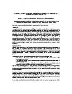
We may model the relationship between the transportation network, the computing nodes with processing resources and the applications used to build services as shown in Figure 1. The model consists of three planes. In the upper plane we have the set of interacting applications. An example of interaction between applications is shown by the solid lines in the application plane. In the bottom plane we have a set of interconnected networks describing the physical connectivity between the applications. The computing nodes where the applications reside, can be seen as the \glue" which binds the distributed application architecture and the network architecture together. Because of the underlying networks, we have virtual all-to-all links on the computing nodes plane. In Figure 1, interaction with other objects in the same plane is shown by the solid lines. Mappings to other planes are shown by the broken lines. Note that the mappings between the three planes may be many-to-many mappings, i.e. one processing node may accommodate several applications and several identical copies of an application may reside at di�erent nodes. 3
Applications
Computing nodes
Networks
Figure 1: The relationship between the transportation networks, the computing nodes and service applications. We will further assume that any application can run on any computing node, subject to the availability of resources for that application. Applications may be moved or copied between nodes with no limitation on how often this may occur. The mapping between applications and processing nodes is therefore dynamic. In many contexts the mapping between computing nodes and the networks will be stable. However, systems are emerging where even the mapping between nodes and networks is dynamic, for example in the form of computing nodes residing in mobile terminals or low orbit satellites. Note that the distributed network model described above is a useful model for the Internet. The upper plane corresponding to the Web; the middle plane representing the servers; and the bottom plane being the international structure of telephone and data networks.
2.3 Distribution transparencies
A set of transparencies is proposed as described in the TINA-C documentation [3, 17], in order to formalize some of the requirements for a distributed network . They are important with respect to the ability to adapt to changes, the availability of services and the exibility in service deployment, provision and management. These transparencies, together with the distributed network model we have described, constitute the basis for the optimization models that are presented below in Sections 3, 4 and 5. � Access transparency. Every application reveals a standardized interface to other applications, independent of where cooperating applications are placed. Applications which together constitute a service can thus be placed on di�erent computers, without this a�ecting the interaction between them and the access they have to each other. 4
� Location transparency. This hides the location of applications from each other.
�
� � �
Applications can interact while their locations change over time, without the other applications noticing it. The system supports mechanisms for locating application instances, and this allows the exible placement of applications over time. Migration transparency. This is an extension to the location and access transparencies above which allows dynamic relocation of application instances. Relocation can take place while services are interacting with each other. This transparency gives us the possibility to completely move an application while it is in use and interacting with other applications. Handover in mobile telecommunication is a typical example. Concurrency transparency. This transparency allows several applications to interact with the same instance of another application at the same time. The fact that other applications use the same instance is hidden. Failure transparency. This makes sure that errors generated by one instance of the application are hidden from other applications and users. Replication transparency. This hides the replication of one application to other computers, from other applications. This means that it is not possible to know which instance of an application we are actually using.
2.4 Abstract infrastructure
The engineering model [17] from TINA-C is used to describe any distributed system as a set of engineering objects interacting through an abstract infrastructure, the Distributed Processing Environment (DPE). This abstract infrastructure exists on every computer in the network and provides a layer between the computer's native computing and communication environment and the services composed of applications. The mechanisms necessary to implement the transparencies above are hidden in the implementation of the DPE. The infrastructure and functionality provided by the DPE is the same for all hardware platforms and all services. The above description of the abstract infrastructure implicitly assumes the existence of some repositories for data storage. We now include a short description of three repositories here, because they justify the validity of the transparencies above, and facilitate understanding of the models that follow later.
� The speci cation repository contains templates for services and interfaces and
identi es the relationships between them. � A trader is a repository which contains information about available interfaces and application instances. Each trader has a domain where it is working and a domain can have several traders. Traders interact with each other to make sure that requests for applications can be met independently of where both the application instances and the users reside. Similarly, they ensure that the applications communicate with the correct interfaces. Hence the traders make it possible to assume that our applications can interact to make a complete service, without knowing each other's location or physical hardware platform. � A relocator keeps track of objects which move while processing. In addition it provides information for the trader that is necessary to nd the requested objects, or alternatively, replicas of it.
5
2.5 Roles
We will identify some of the roles of agents that are found in a distributed network. We only include the roles that have an impact on the models addressed in this paper. The customers are people or software requesting services. New market segments open as service providers are able to o�er services that do not exist today. The capabilities of the new distributed networks together with deregulation suggests that not only will the customers be di�erent from traditional telecom users but the telecom operator's eld of operation can be di�erent. A service provider o�ers services to customers. Providing a service can be done by anyone who has a PC which runs a DPE and is connected to a network. We can therefore assume that the number of service providers will be large and that the differences between traditional software providers and providers of telecommunications services will be blurred and probably disappear. A network provider provides a transportation network with routing and switching capabilities to customers and service providers. Some or all of the network nodes are computing nodes with a DPE. They correspond to computing nodes in Figure 1. The network providers thereby act as hosts for the service providers' applications, both when it comes to computing resources like processing capacity and when it comes to transportation resources. The fall of monopolies and deregulation all over the world opens the possibility of many network and service providers operating in the same market. It is here important to note that a network provider does not necessarily act as a service provider, and the service providers do not necessarily own any of the processing or transmission equipment they use.
3 Service provision The rst model we will consider is that of dynamically allocating the use of processing resources at the computing nodes in order to meet customer requests for services. This should be done to utilize the resources in the best possible way, and may include the option to reject requests. For modelling purposes we will assume in the rest of this paper that the mapping between networks and processing nodes is static. We can then regard a set of processing nodes connected to the underlying networks in a xed manner. Then we have a set of applications which are dynamically allocated to the nodes and connected to each other through the underlying computing nodes and a physical network structure as in Figure 1. Before we completely de ne the problem, we must look closer at the services, how they use resources, and how distribution transparencies in uence resource allocation.
3.1 Services and subservices
Let us rst de ne the term subservice and relate it to services. A service has already been de ned as a set of applications and their required resources. For the purpose of modelling, we now de ne a subservice to be a collection of applications that always run on the same computing node. A subservice can hence be regarded the smallest object we consider for which the distribution transparencies are valid. The other objects included in our models are computers running a DPE, known as the computing nodes, and (complete) services, composed of subservices. If the node has the necessary resources to run the subservice and a decision is made to make it available at the node, the subservice cannot usually be used to 6
meet the demand immediately. There is a setup time in which the subservice can be collected from a speci cation repository, loaded into the memory and initialized, before it can be used to serve requests. We assume that all subservices are available for installment at all nodes. When a subservice is installed at a node, we assume that the only limit on the number of requests that can be served by it, is the node capacity. For a given service we have an estimate of demand: the number of customer requests for the service at the di�erent nodes in the virtual network. The use of the limited resources in the network is described by the use of resources by complete services through the subservices they are composed of. The resource requirement for a given subservice depends on which service is using it. In this paper we assume that the resource use of a subservice increases linearly with the number of customers using it at the same time. In addition the subservice uses a xed amount of the node resources whenever it is installed on the node, even when it is not satisfying a single request. This is a xed resource use induced by having the software running and ready to meet requests in real time. Also note that there may be a delay between the time the service provider decides to remove a service and the time its xed resource use is released.
3.2 Location of demand and transparencies
The distribution transparencies from Section 2.3 indicate that the location of the subservice instances used to meet requests is not important from either the point of view of the interacting subservices or that of the customers. Customers have no preferences when it comes to the service instances they use, but only to the quality of the service. We assume that all nodes have the same capability of running all services. More speci cally the quality of service is not a�ected by properties of di�erent computing nodes. The distribution transparencies therefore give rise to a lot of exibility when it comes to allocating resources in the network, and are crucial to the problem described in this section. The location of subservices clearly does matter when information generated or processed by services is to be transported in the underlying transportation networks. It is exactly in this transportation phase that one of the most important sources for too low quality of service is hidden: namely time delay as a consequence of congested networks. It is natural to assume that the network provider can interact with the service provider to deploy the service to a node nearby the customers, in order to reduce the overhead from the transportation of data. The important question is then if in this setting and given our assumptions, it is sensible to integrate into our decision models representation of the actual underlying cooperation and the information
ows that depend on the allocation of services to the nodes. Even if the inclusion of information ows in service provision models may at rst sight seem necessary, there are several reasons why the opposite can be true. Firstly, in cases where the service provider is not the network provider, an agent o�ering services may not know the physical location of his own subservices, because of migration and replication transparencies. It is also reasonable to believe that service providers, who rent computer capacity from network providers, can use this capacity to set up any service they like. Network providers responsible for the transportation network therefore cannot necessarily control which services are running at which locations. Secondly, a service provider may not know the location of all of the users or even subservices of his service because this information can be hidden by the transparencies and the use of traders. 7
Thirdly, we have indicated that there is a shift in focus, where services go from being mainly transportation oriented to being processing oriented. Inn keeping with the focus of this paper we assume that the processing capacity is the limiting factor, not the transportation. Under the fundamental assumptions that we have a global distributed network where distribution transparencies are valid, and processing capacity is the limiting resource, we have the following strict interpretation of the e�ect of distribution transparencies on resource allocation at an operational level: Demand for processing capacity can be served at any node independent of the location of demand, without reducing quality of service. Based on the above discussion, this would imply the following underlying assumption: We assume that the underlying transportation networks have enough capacity and good enough routing schemes to keep the time delay down on transportation of generated information, independent of the allocation of requests for subservices to nodes in the global network.
It is easy to imagine that the strict interpretation given above can create situations which appear peculiar. For example a typical service request can include two customers and a particular subservice instance. Assume the customers are located in Amsterdam, and the subservice they request is placed in Oslo. If the subservice is mainly transportation of information which is not processed, we can assume that most information is routed locally in the backbone network in the best possible way, without having to pass through Oslo. The subservices that are likely to create strange information ows are the ones that have both a lot of information transported and also processing of the information. The links between the included cities must then be of such capacity that the transportation of information through Oslo does not diminish the quality of service. If this assumption is not valid, the strict interpretation of the e�ect of the transparencies has to be reconsidered. A mild version of the previous assumption can also be presented : In regions of the network, the demand for processing capacity can be served at any node in the region independent of the location of demand, without reducing the quality of service. with the corresponding underlying link capacity assumption: We assume that within regions of the global network, the transportation networks have enough capacity and good enough routing schemes to keep the time delay down on transportation of generated information, independent of the allocation of requests for subservices to nodes. It is important to note that the size of the bounded regions above does not depend on physical distance, but rather the underlying transportation networks of the network providers in question and their alliances. Also note that the regions do not overlap. We notice that under the rst assumption, we only have one such region, namely the whole world. Both of the above assumptions can lead to the models presented in Section 3.3 and Section 3.6. If we believe that the processing capacity at the nodes is the limiting resource, at least the weak interpretation is necessary to fully utilize the possibilities created by the distributed environment for dynamic resource allocation. The main e�ect on modelling the resource allocation from the above, is that both the customer and the service provider are indi�erent to which node meets the 8
demand for a particular request. We do not have to model any information ows generated by a request, only the demand for the services. The actual locations of customers are thus irrelevant to the problem of allocating node resources. This means that the demand for services can be aggregated both over the customers and all the locations in at least a region in the network providing the service.
3.3 A deterministic service provision model
We are now able to specify in more detail the service provider's problem. Let us rst describe a static model assuming deterministic demand and no lead time for installing subservices. The service provider has a set of computers available where he can install subservices. He also faces the demand for the subservices. The problem we want to model here is how to allocate subservices to computing nodes. This is done to best utilize the resources the service provider has available in order to meet the demand for his services. Making available too many subservices at a node means there will be no capacity left to serve the demand for them. Providing too few may imply that there is the capacity to serve demand, but not the ability. Let us here assume that the available amount of the limited resource is large enough to accommodate the requests for all customers, given correct con guration. Complete services are only implicitly included in the model through the resource use of the required subservices. Such an approach is feasible, given the latter assumption that we do not have to reject any customer request. We do not risk rejecting half a request for a complete service (for example sound but not picture in video on demand). Let I be the set of computing (supply) nodes and J the set of subservices (demand nodes). If necessary we use I and J as their cardinality. The zero-one variable z (i; j ) indicates whether or not node i contains subservice j . The capacity reduction associated with installing this service is denoted r(i; j ) and we assume it is in Z+1 . In many cases it is natural to think that the xed resource use is independent of the node so that r(i; j ) = r(j ). The integer variable x(i; j ) denotes the amount of demand for the resource generated by service j and met at node i. The capacity of the resource at node i is s(i) 2 Z+1 . The demand for the limited resource generated by subservice j is �(j ), where we assume �(j ) 2 Z+1 . We rst assume that all parameters de ned above are deterministic. When we require that all demands must be met, the main objective is to nd a feasible solution. This can be modelled as a linear mixed-integer programming problem (MIP) [26]. The feasible region of the deterministic subservice provision problem without rejections is then:
X r(i; j)z(i; j) + X x(i; j) 2J X2J x(i; j)
j
�
j
s(i);
i 2 I;
�(j ); j 2 J ; Mz (i; j ) x(i; j ) � 0; (i; j ) 2 I � J; z (i; j ) 2 B1;x(i; j ) 2 Z+1 ; (i; j ) 2 I � J : The constant M (i; j ) = minfs(i) r(i; j ); d(j )g. The rst two sets of constraints =
2I
i
correspond to classical transportation network constraints with the addition of the supply capacity reduction. The third set of constraints ensures that a processing capacity at a node cannot be used to meet demand for a subservice, unless the subservice is installed there. Integrality requirements on the x variables can be dropped due to the fact that the right-hand side is integer and the constraint matrix is totally unimodular [32] when the z variables are xed. 9
This network is called a Transportation Network with Supply Eating Arcs (TSEA) [10]. We do not give a stochastic version of this model because the following model is strongly related to it, but more relevant. It is interesting to note that the deterministic feasibility problem of TSEA is NP { complete in the strong sense [10]. In this reference an algorithm is also presented to solve the TSEA feasibility problem when r(i; j ) = r(j ).
3.4 Uncertainty
We have mentioned before that one of the main advantages o�ered by the distribution transparencies is the possibility of dynamically changing the resource allocation. This ability to change is even more important when we try to consider uncertainty of demand in our models. Demand is clearly completely inherent in the service provision problem, both in demand and in prices for subservices and rejections. In the treatment of uncertainty here and in the rest of the paper, we use terminology from stochastic programming (see for example [18]). The demand for processing capacity is generated by the demand for complete services. When we map demand from complete services to subservices, we do this by using an estimate of the number of units of processing capacity generated by the service through use of the subservice. The uncertain demand for the resource can then be interpreted in at least three ways:
� A probability distribution for the demand for services is mapped to probability
distributions for the use of resources by the subservices. This is done using the average resource requirement generated through the service's use of the subservices.5 � Deterministic demand for services is mapped to a distribution for resource use, where the resource requirement generated from the services' use of the di�erent subservices is uncertain. � A combination of the two preceding possibilities: a distribution for the services demand is mapped to a probability distribution for resource use through probability distributions for the use of subservices.
The main point is that the distribution of resource use is generated from the estimate of future demand for complete services and their use of resources using the subservices they are composed of. The time frame of this model could be from milliseconds to minutes, depending on the lead time for setting up services and the duration of demand uctuations. We assume that the uncertain parameters are not known when decisions concerning which services to provide at which nodes are taken, but the uncertainty resolves itself during this lead time. When the services are available to meet the demand, we know the values of all uncertain parameters, in particular, we know the demand. The state of the system of computers running services can be described by the current demand for the resource, a list of the running subservices, and a probability distribution of resource use generated by the di�erent subservices at some future point in time. With respect to the demand distributions for complete services, we can make some very useful assumptions. First of all, in most system states the demand distributions imply that there will be no trouble meeting demand. Otherwise, the investment problem is not properly solved. We are not interested in these cases. Instead, we are more interested in cases where there is going to be so much demand for the limited resource that careful planning is necessary to avoid rejections. Such a situation arises when there is an unexpected peak in demand for a service or subservice. 10
Secondly, we assume that only one of the services can peak at any time. This means that in our distributions for the subservice resource use in the next period, we can assume that at most one of the services peaks, or alternatively, that very few of the subservices will be a�ected by the peak. The conditional probability distribution concerning which service, if any, is going to peak in the next time period is based on the system state at the moment, and in particular on the observed tra�c patterns. In the case of discrete distributions, described for example in terms of scenarios, the above discussion indicates that the individual scenarios typically only show peaks in a few of the subservices, depending on which service peaks in that scenario. Some of the subservices may peak in all the scenarios, but some of them will also only be signi cantly a�ected if one speci c service peaks. So, in general, our distribution is such that the di�erences between scenarios can be large. If not, uncertainty would probably not be important.
3.5 Rejection of customers
It is easy to imagine scenarios where the node capacities are too small for the entire demand to be met. This is especially in the case of stochastic demand, but can even occur in the case where the demand is known. In such scenarios we have to allow for some of the customers being rejected. By rejection we mean that the service provider will not meet a request for a service or subservice himself. In practice this means that the customer will have to nd another service provider, or that the service provider or a trader performs this task for him. The last option is more likely to appear when a subservice is rejected that is only part of a complete service that the service provider wants to o�er. In any case there is a cost connected to rejections. In a competitive market we can always assume this cost to be the market price for the rejected subservice. This should be the same for all subservices of equal quality, even for di�erent providers.
3.6 Subservice arrangement under uncertainty
We will now formalize this in a model. In the following, we assume that there is a setup time for a subservice in which it uses the xed capacity requirement, but cannot serve requests. Also when the service provider decides to shut down a subservice, there is a delay before the xed resource use is released. This capacity thus cannot be immediately used to meet demand for other subservices. Let us treat this as a dynamic decision process with two stages and uncertain demand. In the rst stage we decide which subservices to o�er, given uncertain demand. In the second stage uncertainty has resolved, and the subservices we installed are available to meet demand. The following example indicates why uncertainty and dynamics must be included in the model.
Example 1: The e�ect of uncertainty on decisions
As an example assume that we have only one node with a capacity of 200 resource units, and three subservices, (A, B, C) for which there are rejection costs (20, 15, 15) per rejected unit of the resource. The xed resource use when providing the subservices is (40, 20, 10). Uncertain demand for the resource as generated by the subservices, is described by two possible future scenarios, S1 and S2, having equal probability. The demand vector in S1 is (80, 0, 70), and in S2 it is (0, 150, 70). Hence subservice C has a deterministic demand of 70, and either subservice A or subservice B has a peak in demand with a probability of 0:5. Let us rst try to look at this in view of deterministic analysis. In the notation of the preceding model, we say that x = (x(A); x(B ); x(C )) and z = (z (A); z (B ); z (C )). 11
The optimal solution for S1 is z = (1; 0; 1) and x = (80; 0; 70). The rejection cost is 0. The optimal solution for S2 is z = (0; 1; 1) and x = (0; 150; 20). The rejection cost is 750, due to partial rejection of subservice C. This does not give us an implementable solution, because in one case subservice A is installed and in the other subservice B. So what if we use expected demand, (40, 75, 70) as data, and treat it as if it was deterministic when making decisions. The optimal deterministic solution is then to install subservices B and C , and set x = (0; 75; 70) with a rejection cost of 40 � 20 = 800. The rejection cost found in this way does not generally give any indication of the expected rejection cost the decision implies. Because of the uncertainty of demand, the interesting part of this solution is only its rst-stage decision, z . Given that we have subservices B and C installed, we need to minimize the actual rejection costs when uncertainty resolves. In scenario S1 we meet the entire demand for subservice C, meaning x = (0; 0; 70) and in S2 we meet the entire demand for subservice B and as much as possible for subservice C, x = (0; 150; 20). Thus the true expected rejection cost is 0:5 � 80 � 20 + 0:5 � 50 � 15 = 1175 given our decisions from the rst stage. If we instead would have installed subservices A and B , the expected rejection cost would have been 0:5 � 70 � 15 + 0:5 � 70 � 15 = 1050. With A and C installed the expected cost is 0:5 � 0+0:5 � 150 � 15 = 1125. Finally, if we had installed subservices A, B and C the expected rejection cost is 0:5 � 20 � 15 + 0:5 � (20 + 70) � 15 = 825. This is also the solution leading to the minimal expected rejection cost. As we can see the solution we found from deterministic analysis in this case was the worst and gave an expected rejection cost that was 42% higher than the optimal one. Here the possibility of a peak in demand for subservice A and the resulting high rejection cost in this scenario, more than outweighs the expected marginal value of any alternative use of the resource units involved. This was not discovered through deterministic analysis. Now we turn to the mathematical model again. We base the problem formulation on the previous model in Section 3.3 and the above discussion. In the static deterministic case the di�erence from the model in Section 3.3 and the current one is only that we relax the demand constraint by introducing a slack variable t(j ) for every subservice j . This can be interpreted as the rejections. For this deterministic formulation of the problem a large class of facets is known [9]. In the stochastic case prices can be uncertain as well as demand. Let �~(j ) be the cost of rejecting demand for the resource created by subservice j (note that an alternative interpretation is to let �~ represent the di�erence between the price the service provider has to pay to a competitor and the price he obtains from selling the service on the market). If all �(j ) are set to 1 (scaling of equal costs), the objective will be to minimize the number of rejected requests for the resource. To allow rejection of subservices creates some modelling problems since there is no connection in the model to the demand-generating complete services. Therefore we risk rejecting only a part of a complete service for several requests, instead of rejecting entire requests for complete services, as would be natural. To avoid this risk, we have to make some assumptions. In view of the distribution transparencies and the DPE functionality described earlier, it will be reasonable to assume that traders will be able to perform the task of identifying other instances of the subservice that the service provider is not able to o�er, but which can be used by the set of complete services he wants to present to his customers. In short, a request to the trader repository will normally be to ask it to locate a subservice instance owned by him. In cases where this is not possible, the request becomes that of nding this subservice with another service provider. One way of interpreting the above is to say that subservices that are rejected are either hired from other providers, or 12
served in another region of our provider's operating area. The rejection cost can then be interpreted as the cost of getting the subservice elsewhere. Here we give an example of a two-stage formulation of the stochastic service provision problem. Note that the rejection variable t(j ) is eliminated from the formulation. Minimize Q(z )) s:t: r(i; j )z (i; j ) � s(i); i 2 I ;
X
j
2J
z (i; j ) 2 B1 ;
where
(i; j ) 2 I � J ;
Q(z ) = E [q(z )]
where the expectation is taken over the stochastic parameters �~ and �~, and
s.t.
X x(i; j) j
2J
X �(j)[�(j) X x(i; j)] 2J 2I X r(i; j)z(i; j) = s�(i); i 2 I;
q(z ) = min
+
j
i
� s(i) 2J x(i; j ) � Mz (i; j ); x(i; j ) 2 R ;
z
j
(i; j ) 2 I � J ; (i; j ) 2 I � J : The second stage problem is a particularly simple bipartite transportation problem with cost coe�cients only on the arcs used to reject demand. The structure of the objective function can be utilized when solving the model, for example as in [34]. The rst stage is a binary knapsack problem with several independent knapsacks. One should also note that the rst-stage constraints are redundant, since they are represented in a stronger form in the second stage. On the other hand, since the rst-stage constraints imply s� (i) � 0 8i 2 I , this can be regarded as a stochastic integer programming model with relatively complete continues recourse (see for example [18, 35]). 1 +
z
3.7 Extensions of the models
In the previous models we implicitly assumed that the service provider had full knowledge of the sizes of all the available computing nodes. This is not always the case. Another extreme possibility is that he has no knowledge. We can imagine that, in some cases, the network provider who owns the computers on which the subservices are running, is free to replicate and migrate the subservice instances running on his infrastructure. In hiding the complete infrastructure from the service provider, just letting him see it as one node, he is completely free to utilize his resources. Even though the service provider thinks he runs exactly one instance of his subservices, he may in reality run several, and the number and locations may vary over time. The migration and replication is then a choice made by the network provider. The extra induced costs this implies when it comes to xed resource use, is hidden in this case from the service provider by migration and replication transparencies. Still it is reasonable to believe that the service provider should consider the original xed resource use connected to o�ering the service, but only induced once. Alternatively, we can assume that the network provider is free to replicate and migrate instances, and that the service provider pays for all xed resource use. In the rst approach the network provider gets a lot of exibility when it comes to utilizing his resources, by letting the service provider think he has one node available. The 13
price he pays is to cover the cost of replication and migration himself. In the second case the network provider gets the same advantages and the service provider pays. The service provision problem of the rst case is modelled and discussed in [36]. This model is similar to the one in Section 3.6 with only one computing node. Note that the problem for the network provider, including replications and migrations, is equivalent to the model without rejections presented in Section 3.3. It may also be useful to model rejection of requests for complete services. In other words we then model a situation where the service provider is or wants to be the only provider of all or some of the subservices constituting a complete service. Models representing this problem can be found in [36]. In case there are no customer rejections, there is no di�erence from the earlier models. In the preceding two-stage models we have implicitly assumed that two stages are enough to model the detection of a peak in demand, a reaction by allocating services to nodes and time for uncertainty to resolve. There are several reasons why in some cases we may need more than two stages here. Firstly, it is possible that the length of a peak exceeds the lead time of setting up services so that the reallocation of services is possible before the top of the peak is reached. This means that there is increased exibility in the decision process which a two-stage model cannot capture. Secondly, we know that the services can use di�erent subservices in a sequential as well as a parallel manner. This means that the subservices that are used in the beginning of the peak, may be di�erent from the ones used at the end of the peak. Assigning capacity to all these subservices throughout the whole period of decision, may therefore not be a good utilization of the limited resource. The twostage models capture the parallel aspects of subservice use, but not the sequential aspects. Thirdly, we have assumed that before a new peak arrives, there has been enough time for the current one to be handled. If this is not true, more than two time periods may be needed. It is possible to imagine that subservices can be shut down releasing the used capacity immediately. This will in uence the models presented here. Likewise, another approach can be to assume that prior to the peaks in demand, the service system is in a robust state. The goal will then be to meet demand during the peak and return to a robust state with the smallest e�ort of recon guration and reallocation of requests. An initial attempt to model these two variants is given in [36].
4 Node investment We now turn to consider strategic investments in the underlying infrastructure on which we run the services. The area where the network provider operate is divided into non-overlapping regions. We will assume that the regions are given, that distribution transparencies are valid, and that the location of a service inside a region should not in uence the quality of the service to the customer. The regions can for example be similar to the ones we discussed at an operational level in Section 3.2, where processing capacity was the limited resource. Assume that the market for processing capacities is deregulated and competitive, so that several network providers exist. In addition assume that in the market of transportation capacities between regions, we have perfect competition. None of the actors can individually in uence prices of transportation capacities on these links. When facing future demand for services, a network provider must try to plan the capacity of the node resources (for example processing capacity) inside regions. The decisions should ensure that there is enough capacity to meet the demand and 14
at the same time maximize long term pro t. After investments have been made and uncertainty has been resolved, he may have to buy extra processing capacity. On the other hand, he has the option to sell capacity if he over-invested. These are sound assumptions in a deregulated competitive market with many providers. Note that given a high enough quality of the service, distribution transparencies ensure that customers are indi�erent to the location of interacting subservices. The transparencies also makes trading of processing capacity between regions possible. It may then be advantageous to utilize this to deliberately plan processing capacity in such a way that there is a shortage in one region and a surplus in another. This is clearly even more meaningful when demand is uncertain. This trading of capacities between regions, can be considered one of the main issues of investment planning in distributed networks.
4.1 Link capacities
Transportation capacity within regions is not considered here. With given region boundaries and known processing capacities within each region, the problem of deciding link capacities within regions can be regarded as a problem of its own. This problem is of course dependent on the results from the problem we treat here, and also on the solution of the node location problem we treat in the next section. In the models we present here, we assume that the price of building the necessary link infrastructure within the regions is re ected in the investment costs of nodes. It is natural that the cost of the local infrastructure needed increases as the processing capacity in the region increases. In this paper we will assume that the investment costs are linear in the node size. So what is the reason for including link capacities between regions in our models? This stems from recognizing the fact that a lack/surplus of node capacity in one region, may lead to an increase in tra�c between regions. The decision of trading processing capacity between regions at a regular basis, requires that the link between the regions is not a bottleneck. The desired capacity should be available for sending information without a time delay leading to loss of service or a reduced quality of the service. As we have assumed free competition in this market, we know that our decision taker can take the market price to be valid for an, in practice, unlimited amount of information. We still recognize, though, that it is costly to use the links. So if the network provider wants to trade node capacity on the market, he has to pay for the extra induced need for transportation capacity. If we place ourselves as decision-makers at the computing nodes plane in Figure 1, there are virtual all-to-all links for transportation of information between regions. The virtual links may of course also exist as physical links for one or several of the underlying transportation networks. We want to plan how much information we need to transport between regions, as a consequence of trading processing capacity in the market. There are several ways to model the induced information
ows that follows from our network provider's surplus/lack of capacity in a region: 1. Model the ows explicitly, i.e. introduce decision variables for ows between each pair of regions together with variables indicating which surplus region helps out which shortage region. 2. Distribute the induced information ows from regions with surplus/lack of processing capacity to all or some neighbouring regions by a deterministic or average pattern. 3. Model the extra induced information ows from regions with surplus/lack of processing capacity as distributed stochasticly over the links out of the region. 15
In the rst case, the solution of the model will give a strategy for which regions are going to cooperate, and when. This is clearly feasible if we assume that we are only using our own nodes. In the two latter cases we do not explicitly model which surplus areas help out which shortage areas. Therefore, we could say that the shortage of node capacity is covered by buying capacity on the market, and surplus by selling. This seems like a more exible and general approach. It includes the possibility of trading capacity both in the region in question and between this region and others. To be as general as possible, we model the distribution of induced transportation needs from exported/imported node capacities as stochastic parameters as in case 3 above. In our deregulated perfect competition market investment costs in transportation infrastructure should not be directly included in the models. Assume for example that a network provider is of the opinion that the market prices he has been given for future transportation capacity is too high. He may then claim that he will invest himself and face lower prices than the ones present in the market. This may be so, but he should still use the market price as an estimate of the cost of sending information between regions when he plans his node capacities. In the perfect competition market we have assumed, the pro t he can get from investments in transportation capacity is independent of his investments in nodes. Hence it should also be treated independently as an investment of its own, and implemented if pro table. When we base our decisions concerning need for transportation capacities solely on market prices, we need to include some market mechanisms. We have to di�erentiate between buying capacity at the spot-market and making long term contracts having a xed price with transportation capacity suppliers. The latter possibility eliminates uncertainty concerning the price of transportation capacity for the agreed on use of a virtual link.
4.2 Uncertainty
The following parameters may be uncertain: The demand for processing and link capacities, prices of capacities in the future spot-market and the information ows induced by surplus/shortage of processing capacity in the regions. In this paper we regard transportation costs as known if contracted at the rst stage. Similarly investments costs for node capacity is deterministic, as a consequence of using o�shelf equipment only. We have earlier shown how demand-uncertainty in uences decisions in the service provision problem. In particular we stressed the negative e�ect of not utilizing
exibility when decisions are made. When it comes to dimensioning processing capacity and estimating the need of link capacity at a strategic level, long term demand-uncertainty is important. Flexibility in trading capacity on the market after uncertainty has resolved, cannot be captured by deterministic analysis. In recognition of the importance of uncertainty for these types of decisions, we will therefore go directly to a stochastic model.
4.3 Model for investment in nodes
In the modelling example given here, we will assume that all costs of capacity increase linearly with the used capacity. This is the case if we assume perfect competition on the markets for processing as well as for transportation capacities. Our decision-maker can assume the prices to be valid independent of his and other individual agents decisions. In the rst stage of the model we invest in nodes and contract link capacity. In the second stage we face the uncertain demand for processing and between-region 16
link capacity. Spare capacity can be sold on the market. If capacity is too low, we will need to buy more capacity on the market. In both cases we may generate transportation ows out of or into our region. We now present a stochastic two-stage model. In the following, we use E to denote the set of possible combinations of (i1 ; i2 ) 2 I � I where i1 6= i2 . First stage: min
X f (y(i))y(i) + X 2I
2E
s.t.
c(i1 ; i2 )l(i1 ; i2 ) + Q(l; y)
(i1 ;i2 )
i
(l; y) 2 S ; l(i1; i2 ) 2 R1+ ; y(i) 2 Z+1 ;
8(i ; i ) 2 E ; 8i 2 I ; 1
2
where l(i1; i2 ) is the contracted capacity on the virtual link between i1 and i2 , and c(i1 ; i2 ) is the corresponding deterministic price. The size of the computers in region i, is denoted by the integer variable y(i) (if the upper bound on this variable is large, it may be considered a real decision variable). Here f (i) is the investment cost in region i. The constraint set for our rst decisions is de ned in the feasible region S. The function Q is the expected value function of the second stage problem,
Q(l; y) = E [q(l; y)] �~.
where the expectation is taken over the stochastic parameters �~; ~; �~; !~ ; �~; �~ and The second stage is:
X[ �(i)�(i) + �(i)x(i) X2I !(i ; i )[p(i ; i ) +
q(l; y) =min
i
2E
1
2
1
2
�(i)x(i)+ ] p(i1 ; i2 )+ ]
(i1 ;i2 )
s.t.
x(i) x+ (i) =�(i) y(i); p(i1 ; i2 ) p(i1; i2 )+ �1 (i1 ; i2 )x(i1 )+ �2 (i1 ; i2 )x(i2 ) = (i1 ; i2 ) l(i1 ; i2 ); p(i1 ; i2 )+ ; p(i1 ; i2 ) 2 R1+ ; (i1 ; i2) 2 E x(i) 2 R1+ ; i 2 I :
i 2 I; (i1 ; i2 ) 2 E ;
The rst constraint set concerns the processing capacities of the nodes. The variables x(i) =x(i)+ represent the processing capacity shortage and surplus in region i. The stochastic parameter �~(i) is the future processing capacity need in region i. The �~(i) is the uncertain pro t per demanded capacity unit. Further �~(i) and �~(i) are respectively the cost and revenue experienced if processing capacity is too small in region i. The second constraint set concerns the transportation capacities on the virtual links. Here p+ =p is the surplus/shortage for transportation capacity on virtual links between di�erent regions. Here !~ is the price when buying and selling link capacity on the market. The demand for capacity on the virtual link between i1 and i2 is given by ~(i1 ; i2). Parameters �~1 and �~2 describe how surplus and shortage capacity in the nodes induce transportation needs. These parameters can be stochastic. If we look at the term �� in the second stage objective, we notice that it is a random constant, namely our pro t when meeting the demand for resource capacity. 17
From an economical point of view this term is crucial because it is normally what gives a positive result. From an optimization point of view, this stochastic constant term can be omitted. The rst-stage objective can be adjusted by its expected value to give the real cost. Implicitly in this objective is the fact that a network provider will meet the demand he actually gets for capacity. If this is more than he has available, he will have to buy capacity on the market. It is implicit in the formulation that it will always be useful to fully utilize the processing capacity of the nodes. If �~1 = �~2 the model has two stages with an integer rst stage and simple continues recourse in the second, see for example [18, 35]. Otherwise the model has relatively complete recourse.
4.4 Extensions to the model
Multistage models are better suited if the uncertainty gradually resolves over time and we are able to change our plans based on this increased knowledge. In that case the two-stage model we have presented is not able to capture the exibility inherent in the decision process. If we do not believe in, or do not want to enforce, the above requirement of trading processing capacity between regions, we can omit to plan the use of link capacities between regions in our model. This still assumes that we are trading processing capacity in the market, but only inside the region where we have surplus/lack of capacity. Clearly, the transportation capacity needs on links between the regions are still important, but the decisions we are modelling are no longer connected. The di�erence from above, is that we now assume that the trading of capacity does not introduce extra capacity needs on links between regions. These links should therefore not be handled together with strategic planning of node capacities. An example of such a model can be found in [36]. We assumed here that the market for transportation capacities between regions has perfect competition. If this is not the case, we have to study more carefully prices for transporting information over a virtual link. Especially we have to examine the real physical underlying networks. Investment decisions in transportation infrastructure may now change market prices. This extension is not trivial. Remember that one computing node, may be mapped to several networks. There are several providers of network infrastructure. Our network provider planning his node capacities, may himself be one of them. It is here important to realize that there is dynamic (re)allocation of resources in the physical packet switched transportation networks underneath the computing nodes. Several di�erent network paths and providers can be utilized simultaneously to send information between the regions in question. It is clear that there is no direct mapping between the capacity need of a virtual link and the underlying physical networks. This implies that the price of transportation capacity experienced by our decision-maker between two regions, may not in general be treated independently from the other node providers investments, their capacity needs and their prices. In addition a single virtual link can in general not be treated isolated when making decisions concerning capacity in the network.
5 Node location problem As we will see, the node location problem is related to the problem above but can also be viewed in its own right. Consider a xed number of sites where computers can be installed inside a bounded region of our network. The purpose of these computers is to meet demand for processing capacity within the region. We also 18
assume that each site has a cost/pro t associated with o�ering a subservice to customers located at di�erent places in the region, and an investment cost, or xed cost, for putting a computer there. At each site the network provider can choose between computers of di�erent sizes and types. He wants to locate the processing capacity in the region so as to minimize the cost of installing enough processing and link capacity to meet the overall demand. Obviously di�erent choices of node sites can lead to di�erent costs for meeting subservice demand, both as a consequence of investments made in the transportation infrastructure and as a consequence of di�erent operating costs. In the previous section we presented a model which provided an answer to the question of how large the overall capacity in each region should be. The solution of that problem can be included in the node location problem as the lower bounds for the region's installed capacity. It is natural to assume that the regions in question here are the same as those in the previous problem and the ones discussed at an operational level in Section 3.2. In the same way as earlier, we assume that processing capacity is the limiting resource, and that distribution transparencies are valid. We must include the possibility of handling demand that exceeds the installed capacity. This can be done by allowing rejections or trading of processing capacity on the market.
5.1 Transparencies, link capacities and demand
How do we de ne customers and their locations? Subservices are often requested as an interaction between two or more customers, possibly at di�erent locations. We let all virtual links between possible sites in the network correspond to locations of requests for subservices. We also have the demand which is present at a single location, re ecting the situation that the sites where we can put computers are also locations of demand. Note that many subservices bring about interactions between more than two locations. The request would in this case contribute to demand for the subservice over all links included in the request. In the overall problem we consider only aggregated demand at each virtual link, but we are able to identify which subservices generate that demand. We can now specify which part of the demand for the various subservices at the di�erent locations is to be met at each particular site. It is here important to see how this ts the technological framework we de ned earlier in Section 2. When processing was the limiting factor, transportation transparencies made it possible to conclude in Section 3.2 that the location of demand inside regions was not important at the operational level. We will now try to minimize a cost of meeting demand that is dependent on the locations. If we consider strategic or tactical planning, there is no doubt that the location of nodes relative to demand matters. A major reason for this is precisely the exibility in resource allocation at the nodes that the transparencies introduce at the operational level and the corresponding need for transportation capacities. There are at least two di�erent ways of including this in the model:
� We can explicitly model the links between customer locations and their capacity and installment costs. � In the price of meeting demand for subservices from a given site, we include the cost of the necessary transportation infrastructure generated by this choice.
The last approach is selected because there is an enormous amount of e�ort already put into models for transportation network design. Given the location of sites, their sizes, and the type/amount of demand we expect at the sites, the 19
problem of designing the underlying transportation network is extensively treated in the literature, see for example [13, 15, 16, 25, 29, 33]. The investment costs of the local transportation infrastructure, can probably be split in one xed part depending on the node site (and size) and one variable part depending on the actual use of the node. We assume in the following that the price of meeting demand for a subservice from a given site indicates both operational costs and the variable part of necessary investments in the underlying infrastructure. This infrastructure must be of such a quality and capacity that when transparencies are valid at an operational level, the quality of service is independent of the locations of the subservices within the region. Likewise we include in the investment cost for a node the xed part of necessary investments in local transportation infrastructure.
5.2 Interpretation of the chosen approach
The allocation of subservices to sites must not be confused with the allocation we have already studied at an operational level. The purpose here is just to ensure that the overall demand for processing capacity can be met. We also recognize the fact that the total demand for processing capacity, or even the demand for special subservices, is not necessarily equally distributed over the region. If, at a tactical level, we say that a node must have a given size to be able to house a speci c subservice, this implies that we will dimension the underlying transportation infrastructure based on this. One should here note that this assignment is not xed and is certainly not identical to the assignment of subservices to nodes at an operational level. We may then instead choose to hide the identity of subservices and model the demand for processing capacity aggregated over all subservices at a location. However, this is just a special case of the rst approach, and we will therefore treat the rst.
5.3 The node location model
The important uncertain factors are the demand for subservices (given in terms of resource use) and the prices of meeting this demand from di�erent locations. Both operational and investment costs are included in these prices. As in the problems presented previously, we need a stochastic dynamic model to describe the exibility in the decision process and treat the uncertainty. The problem can be formulated as a capacitated facility location model. There are several ways of modelling this problem. References [12, 19] give overviews of di�erent formulations and contain a lot of references. The model given here is an example of one modelling approach. The computers are the facilities, the underlying network links are the customer locations, and demand for the subservices over the links should be met to maximize pro t/minimize cost subject to capacity constraints on the nodes. Let y(i) be 1 if computer i is installed and 0 otherwise. The corresponding investment cost is f (i). It is natural to assume that the capacity of the computers is limited. We denote by U (i) the capacity of computer i. Let U be the overall amount of capacity the network provider at least need to install in the region, and U the maximum. The lower bound may come from investment models treated earlier and the upper bound is possibly absent. The variable x(i; j; e) is the demand for the resource generated by subservice j over link e that we decide to meet at node i. The set of all links is E . The demand for the resource generated by subservice j over link e is named �~(e; j ). We denote the possibly stochastic cost/pro t of meeting the demand for subservice j over link e at node i as �~(i; j; e). This parameter should include the variable cost of installing or renting infrastructure in the backbone network. As we have argued, this cost l
u
20
may be independent of subservices. In this formulation we have assumed that it is linear in the use of processing capacity. The variable t(j ) describes how many resource units demanded for subservice j we choose not to meet. The rejection cost (or, alternatively, the cost of obtaining the subservice on the market, for example, from another region) is given by �~(j ). The corresponding stochastic two-stage model can be written as follows. First stage:
X f (i)y(i) + Q(y) 2I X U � U (i)y(i) � U
min
i
l
i
u
2I
Q(y) = E [q(y)]
where the expectation is taken over the stochastic parameters �~; �~ and �~. Second stage:
q(y) = min
X X X �(i; j; e)x(i; j; e) + X X �(j)t(e; j) 2I 2J 2E
i
s.t.
j
e
j
X x(i; j; e) +x(ti;(e;j; ej))=���((e;e; jj))y; (i); 2I X X x(i; j; e)�U (i); i
j
2J 2E e
x(i; j; e) 2 R1+ ; y(i) 2 B1;
2J 2E e
8(i; j; e) 2 I � J � E ; 8e; j 2 E � J ; 8i 2 I ; 8(i; j; e) 2 I � J � E ; 8i 2 I :
Some references for the stochastic facility location problem are [4, 11, 21, 22, 23, 20].The formulation above is a stochastic integer programming model with binary rst stage and relatively complete continues recourse, see for example [18, 35].
5.4 Extensions of the model
When uncertainty concerning demand resolves over time, a two-stage model may not be able to describe the implied exibility this gives with respect to waiting before full capacity is installed. To completely capture the dynamics of this problem, may require more than two time periods.
6 Conclusions We rst identi ed the need for optimization models by considering distributed and processing oriented aspects of a telecommunications network. The main reason for this is the introduction of new technology and a shift in the focus of the services provided in the network from data transport to information processing. The models we presented were based on a distributed telecommunications framework de ned by TINA-C[6, 30]. The distribution transparencies and the abstract infrastructure de ned here are crucial for models treating service provision and investment in distributed networks. The paper discusses decisions for operational resource allocation at the service providing processing nodes, investment in processing and transportation capacity and decisions concerning how to distribute processing capacity in a region of the network. 21
The models presented in this paper are above the transportation level of the network. They do not treat detailed design of the transportation network underneath, but rather include the relations between the distributed computing nodes providing services and the actual data transported, through the prices and the markets for transportation capacity. From the technological framework of TINA-C, and given the assumption that processing capacity is the limited resource in our network, we conclude that, in regions of the network, allocation of computer resources to services at an operational level may be made independent of the location of the demand. In requiring this, we utilize the increased exibility for dynamically allocating resources in a distributed network. Increased exibility clearly in uences the decisions to be made for investments in infrastructure, both when it comes to processing and transportation capacities. Strategic and tactical decision models for distributed telecommunication networks, hence cannot be studied isolated from models concerning dynamic resource allocation and the assumptions they are based on. A shift in focus at the operational level from transportation of data to processing of information is also bound to present a need for modelling new aspects when it comes to investments. Examples of how some of these new aspects can be treated and assumptions underlying them are given in this paper. The paper considers both operational, tactical and strategic decisions, and relate them to each other.
7 Future work The models presented are an introduction to how modelling new aspects of distributed networks could be achieved. Several of the models have suggested extensions that may make them a closer match to the real world we are trying to describe. This is true both when it comes to the technological aspects and modelling the underlying dynamic decision process. Work put into future model development may be devoted to nding the best ways to model various aspects, given the reasons for the models. But we should also try to describe alternative models focusing on di�erent aspects of distributed networks. There is no e�cient general method for solving stochastic integer programs. As for deterministic integer programming, tailored algorithms and solution methods are necessary to solve the models. This is going to be the main area of work on the above models in near future. Also it is clear that a lot of work remains when it comes to describing the underlying stochastic features of our problems. Finding the necessary data and their probability distributions is critical for the results the models give, and their usefulness. Another area of interest is the problem with the availability of data. The models presented incorporate decision making for a future distributed communications network. The data needed are often uncertain at the point of decision. Because these models also describes a reality and a functionality of networks that are not present today, the availability of data is also uncertain. Work remains to be done both when it comes to de ning what data we should assume are available and how to collect the data.
22
References [1] S. Aggarwal, J. A. Garay, and A. Herzberg. Adaptive video on demand. Manuscript. [2] E.C. Anderson and N. Natarajan. A reference architecture for telecommunications operations applications. Journal of Network and Systems Management, 1(3), 1993. [3] J.A. Audestad. Lecture notes. Course 45356 Communication in distributed systems, Department of Computer Systems and Telematics, UNIT/NTH, 7034 Trondheim, Norway, 10.10.1995. [4] J. Balachandran and S. Jain. Optimal facility location under random demand with general cost structure. Naval Research Logistics Quarterly, 23:421{436, 1976. [5] A. Bar-Noy, J.A. Garay, and A. Herzberg. Sharing video on demand-constant competitive ratio with long noti cation time. In 3rd Annual European Symp. On Algorithms, LNCS (979), pages 538{553, Corfu, Greece, September 1995. Springer-Verlag. [6] W.J. Barr, T. Boyd, and Y. Inoue. The TINA initiative. IEE Communications Magazine, pages 70{76, March 1993. [7] N. Chapman and S. Montesi. Overall concepts and principles of TINA. Document no. TB MDC.018 1.0 94, TINA-C, February 1995. [8] M. De Prycker. Asynchronous Transfer Mode, Solution for Broadband ISDN. Prentice Hall, New Jersey, 1995. [9] S. Dye, L. Stougie, and A. Tomasgard. Relaxations and valid inequalities for the service provision problem. In preparation. [10] S. Dye, A. Tomasgard, and S.W. Wallace. Feasibility in transportation networks with supply eating arcs. Accepted in Networks. [11] P.M. Franca and H.P.L. Luna. Solving stochastic transportation-location problems by generalized Benders decomposition. Transportation Science, 16:113{ 126, 1982. [12] R.L. Francis, L.F. McGinnis, and J.A. White. Locational analysis. European Journal of Operational Research, 12(3):220{252, 1983. [13] A.A. Gaivoronski. Robust access planning for ATM network in the presence of uncertain multiservice demand. In NETWORKS`94 \Planning for a customerresponsive network", September 1994. [14] B. Gavish and I. Neuman. Routing in a network with unreliable components. IEEE Transactions on Communications, 40(7):1248{1258, 1992. [15] B. Gavish, editor. Operations research in telecommunications. Annals of Operations Research, 36:402 pages, 1992. [16] B. Gavish, editor. Special issue on telecommunications systems: Modeling, analysis and design. Operations research, 43(1):29{191, 1995. [17] P. Graubmann, W. Hwang, M Kudela, K. MacKinnon, N. Mercouro�, and N. Watanebe. Engineering modelling concepts (DPE architecture). Document no. TB NS.005 2.0 94, TINA-C, 1994. 23
[18] P. Kall and S.W. Wallace. Stochastic Programming. Wiley, Chichester, 1994. [19] M. Labbe and F.V. Louveaux. Location problems. Discussion paper, Institut de Statistique, Universite Libre de Bruxelles, Belgium, July 1996. [20] G. Laporte, F.V. Louveaux, and L. Van Hamme. Exact solution of a stochastic location problem by the L-shaped algorithm. Transportation Science, 28:95{ 103, 1994. [21] L.J. Le Blanc. A heuristic approach for large scale discrete stochastic transportation-location problems. Computers and Mathematics with Applications, 3:87{94, 1977. [22] F.V. Louveaux. Discrete stochastic location models. Annals of Operations research, 6:23{34, 1986. [23] F.V Louveaux and D. Peeters. A dual-based procedure for stochastic facility location. Operations research, 40:564{573, 1992. [24] S. Mullender, editor. Distributed Systems. Addison-Wesley, New York, 1993. [25] P. Nain and K.W. Ross, editors. Stochastic modelling of telecommunication systems. Annals of Operations Research, 35:357 pages, 1992. [26] G. L. Nemhauser and L. A. Wolsey. Integer and Combinatorial optimization. Wiley-Interscience series in discrete mathematics and optimization. Wiley, New York, 1988. [27] G. Nilsson, F. Dupuy, and M. Chapman. An overview of the Telecommunications Information Networking Architecture. In TINA 95 Conference, Melbourne, Australia, P1, 1995. [28] R. Onvural. Asynchronous Transfer Mode Networks: Performance Issues. Artech House, Boston, 1994. [29] R.O. Onvural, H.G. Perros, and G. Pujolle, editors. Methodologies for high speed networks. Annals of Operations Research, 49:373 pages, 1994. [30] T. Rowbotham. The TINA Consortium { A Collaborative Way Forward. In TELECOM 95, Geneva, 1995. [31] H. Rubin and N. Natarajan. A distributed software architecture for telecommunication networks. IEEE Network Magazine of Computer Communication, January/February 1994. [32] A. Schrijver. Theory of linear and integer programming. Interscience series in discrete mathematics and optimization. Wiley, New York, 1986. [33] Suvrajeet Sen, Robert D. Doverspike, and Steve Cosares. Network planning with random demand. Telecommunications Systems, 3:11{30, 1994. [34] L. Stougie, A. Tomasgard, and M.H. van der Vlerk. Some approaches for solving the stochastic service provision problem. In preparation. [35] L. Stougie and M.H. van der Vlerk. Stochastic integer programming. In M. Delamico, F. Ma�oli, S. Martello (editors), Combinatorial Optimization: Annotated Bibliographies, Wiley, Chichester, To appear.
24
[36] A. Tomasgard, S. Dye, S.W. Wallace, J.A. Audestad, L. Stougie, and M.H. van der Vlerk. Stochastic optimization models for distributed communication networks. Working paper, Department of industrial economics and technology management, Norwegian University of Science and Technology,7034 Trondheim, Norway, 1997.
25