Low overhead analysis of large distributed data sets is necessary for current ... To analyze large data sets, it is common practice to employ classification [6]: In ...
Distributed Data Classification in Sensor Networks Ittay Eyal Idit Keidar Raphael Rom Department of Electrical Engineering, Technion — Israel Institute of Technology
Abstract Low overhead analysis of large distributed data sets is necessary for current data centers and for future sensor networks. In such systems, each node holds some data value, e.g., a local sensor read, and a concise picture of the global system state needs to be obtained. To this end, we define the distributed classification problem, in which numerous interconnected nodes compute a classification of their data, i.e., partition these values into multiple collections, and describe each collection concisely. We present a generic algorithm that solves the distributed classification problem and may be implemented in various topologies, using different classification types. For example, the generic algorithm can be instantiated to classify values according to distance, like the famous k-means classification algorithm. However, the distance criterion is often not sufficient to provide good classification results. We present an instantiation of the generic algorithm that describes the values as a Gaussian Mixture (a set of weighted normal distributions), and uses machine learning tools for classification decisions. We prove that any implementation of the generic algorithm converges over any connected topology, classification criterion and collection representation, in fully asynchronous settings.
1
Introduction
To analyze large data sets, it is common practice to employ classification [6]: In classification, the data values are partitioned into several collections, and each collection is described concisely using a summary. This classical problem in machine learning is solved using various heuristic techniques, which typically base their decisions on a view of the complete data set, which is stored in some central database. However, it is sometimes necessary to perform classification on data sets that are distributed among a large number of nodes. For example, in a grid computing system, load balancing can be implemented by having heavily loaded machines stop serving new requests. But this requires analysis of the load of all machines. If, e.g., half the machines have a load of about 10%, and the other half is 90% utilized, the system’s state can be summarized by partitioning the machines into two collections — lightly loaded and heavily loaded. A machine with 60% load is associated with the heavily loaded collection, and should stop taking new requests. But, if the collection averages were instead 50% and 80%, it would have been associated with the former, i.e., lightly loaded, and would keep serving new requests. Another scenario is that of sensor networks with thousands of nodes monitoring conditions like seismic activity or temperature [1, 17]. In both settings, there are strict constraints on the resources devoted to the classification mechanism. Largescale computation clouds allot only limited resources to monitoring, so as not to interfere with their main operation, and sensor networks use lightweight nodes with minimal hardware. These constraints render the collection of all data at a central location infeasible, and therefore rule out the use of centralized classification algorithms. In this paper, we address the problem of distributed classification. To the best of our knowledge, this paper is the first to address this problem in a general fashion. A more detailed account of previous work appears in Section 2, and a formal definition of the problem appears in Section 3. A solution to distributed classification ought to summarize data within the network. There exist distributed algorithms that calculate scalar aggregates, such as sum and average, of the entire data set [11, 8]. In contrast, a classification algorithm must partition the data into collections, and summarize each collection separately. In this case, it seems like we are facing a Catch-22 [10]: Had the nodes had the summaries, they would have been able to partition the values by associating each one with the summary it fits best. Alternatively, if each value was labeled a collection identifier, it would have been possible to distributively calculate the summary of each collection separately, using the aforementioned aggregation algorithms. In Section 4 we present a generic distributed classification algorithm to solve this predicament. Our algorithm captures a large family of algorithms that solve various instantiations of the problem — with different approaches to classification, classifying values from any multidimensional domain and with different data distributions, using various summary representations, and running on arbitrary connected topologies. In our algorithm, all nodes obtain a classification of the complete data set without actually hearing all the data values. The double bind described above is overcome by implementing adaptive compression: A classification can be seen as a lossy compression of the data, where a collection of similar values can be described succinctly, whereas a concise summary of dissimilar values loses a lot of information. Our algorithm tries to distribute the values between the nodes. At the beginning, it uses minimal compression, since each node has only little information to store and send. Once a significant amount of information is obtained, a node may perform efficient compression, joining only similar values. For example, a common approach to classification summarizes each collection by its centroid (average of the values in the collection) and partitions the values based on distance. Such a solution is a possible implementation of our generic algorithm. Since the summary of collections as centroids is often insufficient in real life, machine learning solutions typically also take the variance into account, and summarize samples as a weighted set of Gaussians (normal distributions), which is called a Gaussian Mixture (GM) [16]. In Section 5, we present a novel distributed classification algorithm that employs this approach, also as an instance of our generic algorithm. The GM 1
algorithm makes classification decisions using a popular machine learning heuristic, Expectation Maximization (EM) [5]. We present in Section 5.3 simulation results showing the effectiveness of this approach. The centroids and GM algorithms are but two examples of our generic algorithm; in all instances, nodes independently strive to estimate the classification of the data. This raises a question that has not been dealt with before: does this process converge? One of the main contributions of this paper, presented in Section 6, is a formal proof that indeed any implementation of our generic algorithm converges, s.t. all nodes in the system learn the same classification of the complete data set. We prove that convergence is ensured under a broad set of circumstances: arbitrary asynchrony, an arbitrary connected topology, and no assumptions on the distribution of the values. Note that in the abstract settings of the generic algorithm, there is no sense in defining the destination classification the algorithm converges to precisely, or in arguing about its quality, since these are applicationspecific and usually heuristic in nature. Additionally, due to asynchrony and lack of constraints on topology, it is also impossible to bound the convergence time. In summary, this paper makes the following contributions: • It formally defines the problem of classification in a distributed environment (Section 3). • It provides a generic algorithm that captures a range of algorithms solving this problem in a variety of settings (Section 4). • It provides a novel distributed classification algorithm based on Gaussian Mixtures, which uses machine learning techniques to make classification decisions (Section 5). • It proves that the generic algorithm converges in very broad circumstances, over any connected topology, using any classification criterion, in fully asynchronous settings (Section 6).
2
Related Work
Kempe et al. [11] and Nath et al. [14] present approaches for calculating aggregates such as sums and means using gossip. These approaches cannot be directly used to perform classification, though this work draws ideas from [11], in particular the concept of weight diffusion, and the tracing of value weights. In the field of machine learning, classification has been extensively studied for centrally available data sets (see [6] for a comprehensive survey). In this context, parallelization is sometimes used, where multiple processes classify partial data sets. Parallel classification differs from distributed classification in that all the data is available to all processes, or is carefully distributed among them, and communication is cheap. Centralized classification solutions typically overcome the Catch-22 issue explained in the introduction by running multiple iterations. They first estimate a solution, and then try to improve it by re-partitioning the values to create a better classification. K-means [13] and Expectation Maximization [5] are examples of such algorithms. Datta et al. [4] implement the k-means algorithm distributively, whereby nodes simulate the centralized version of the algorithm. Kowalczyk and Vlassis [12] do the same for Gaussian Mixture estimation by having the nodes distributively simulate Expectation Maximization. In contrast to this paper, they require multiple iterations to obtain their estimation, since the entire data set is required for re-partitioning. Moreover, they demonstrate convergence through simulation only, but do not provide a convergence proof. Haridasan and van Renesse [9] and Sacha et al. [15] estimate distributions in sensor networks by estimating histograms. Unlike this paper, these solutions are limited to single dimensional data values. Additionally, both use multiple iterations to improve their estimations. While these algorithms are suitable for certain distributions, they are not applicable for classification, where, for example, small sets of distant values should not be merged with others. They also do not prove convergence. 2
3
Model and Problem Definitions
3.1
Network Model
The system consists of a set of n nodes, connected by communication channels, s.t. each node i has a set of neighbors neighborsi ⊂ {1, · · · , n}, to which it is connected. The channels form a static directed connected network. Communication channels are asynchronous but reliable links: A node may send messages on a link to a neighbor, and eventually every sent message reaches its destination. Messages are not duplicated and no spurious messages are created. Time is discrete, and an execution is a series of events occurring at times t = 0, 1, 2, · · · .
3.2
The Distributed Classification Problem
At time 0, each node i takes an input vali — a value from a domain D. In all the examples in this paper, D is a d-dimensional Cartesian space D = Rd (with d ∈ N). However, in general, D may be any domain. A weighted value is a pair hval, αi ∈ D × (0, 1], where α is a weight associated with a value val. We associate a weight of 1 to a whole value, so, for example, hvali , 1/2i is half of node i’s value. A set of weighted values is called a collection: Definition 1 (Collection). A collection c is a set of weighted values with unique values. The collection’s ∆ P weight, c.weight, is the sum of the value weights: c.weight = hval,αi∈c α. A collection may be split into two new collections, each consisting of the same values as the original collection, but associated with half their original weights. Similarly, multiple collections may be merged to form a new one, consisting of the union of their values, where each value is associated with the sum of its weights in the original collections. A collection can be concisely described by a summary in a domain S, using a function f that maps collections to their summaries: f : (D × (0, 1])∗ → S. The domain S is a pseudo-metric space (like metric, except the distance between distinct points may be zero), with a distance function dS : S 2 → R. A collection c may be partitioned into several collections, each holding a subset of its values and summarized separately1 . The set of weighted summaries of these collections is called a classification of c. Weighted values in c may be split among collections, so that different collections contain portions of a given value. The sum of weights associated with a value val in all collections is equal to the sum of weights associated with val in c. Formally: Definition 2 (Classification). A Classification C of a collection c into J collections {cj }Jj=1 is the set of weighted summaries of these collections: C = {hf (cj ), cj .weighti}Jj=1 s.t. J X X X ∀val : α = α . j=1
hval,αi∈c
hval,αi∈cj
A classification of a value set {valj }lj=1 is a classification of the collection {hvalj , 1i}lj=1 . The number of collections in a classification is bounded by a system parameter k. A classification algorithm maintains at every time t a classification classificationi (t), yielding an infinite series of classifications. For such a series, we define convergence: 1
Note that partitioning a collection is different from splitting it, because, when a collection is split, each part holds the same values.
3
Definition 3 (Classification Convergence). A series of classifications n o∞ t {hf (cj (t)), cj (t).weighti}Jj=1
t=1
converges to a destination classification, which is a set of l collections {destx }lx=1 , if for every t ∈ 0, 1, 2, · · · there exists a mapping ψt between the Jt collections at time t and the l collections in the destination classification ψt : {1, · · · , Jt } → {1, · · · , l}, such that: 1. The summaries converge to the collections to which they are mapped by ψt : � t→∞ max dS (f (cj (t)), f (destψt (j) )) −−−→ 0 . j
2. For each collection x in the destination classification, the relative amount of weight in all collections mapped to x converges to x’s relative weight in the classification: P destx .weight {j|ψt (j)=x} cj (t).weight t→∞ ∀1 ≤ x ≤ l : . −−−→ Pl PJt j=1 cj (t).weight y=1 desty .weight We are now ready to define the problem addressed in this paper, where a set of nodes strive to learn a common classification of their inputs. As previous works on aggregation in sensor networks [11, 14, 2], we define a converging problem, where nodes continuously produce outputs, and these outputs converge to such a common classification. Definition 4 (Distributed Classification Problem). Each node i takes an input vali at time 0 and maintains a classification classificationi (t) at each time t, s.t. there exists a classification of the input values {vali }ni=1 to which the classifications in all nodes converge.
4
Generic Classification Algorithm
We now present our generic algorithm that solves the Distributed Classification Problem. At each node, the algorithm builds a classification, which converges over time to one that describes all input values of all nodes. In order to avoid excessive bandwidth and storage consumption, the algorithm maintains classifications as weighted summaries of collections, and not the actual sets of weighted values. It begins with a classification of its own input value. It then periodically splits its classification into two new ones, which have the same summaries but half the weights of the originals; it sends one classification to a neighbor, and keeps the other. Upon receiving a classification from a neighbor, a node merges it with its own, according to an application-specific merge rule. The algorithm thus progresses as a series of merge and split operations. In Section 4.1, we present the generic distributed classification algorithm. It is instantiated with a domain S of summaries used to describe collections, and with application-specific functions that manipulate summaries and make classification decisions. As an in-line example, we present an algorithm that summarizes collections as their centroids — the averages of their weighted values. In Section 4.2, we enumerate a set of requirements on the functions the algorithm is instantiated with. We then show that in any instantiation of the generic algorithm with functions that meet these requirements, the weighted summaries of collections are the same as those we would have obtained, had we applied the algorithm’s operations on the original collections, and then summarized the results. 4
4.1
Algorithm
The algorithm maintains at each node an estimate of the classification of the complete set of values. Each collection c is stored as a weighted summary. By slight abuse of terminology, we refer by the term collection to both a set of weighted values c, and its summary–weight pair hc.summary, c.weighti. The algorithm for node i is shown in Algorithm 1 (at this stage, we ignore the parts in dashed frames). The algorithm is generic, and it is instantiated with S and the functions valToSummary, partition and mergeSet. The functions of the centroids example are given in Algorithm 2. The summary domain S in this case is the same as the value domain, i.e., Rd . Initially, each node produces a classification with a single collection, based on the single value it has taken as input (Line 2). The weight of this collection is 1, and its summary is produced by the function valToSummary : D → S, which encapsulates f . In the centroids example, the initial summary is the input value (Algorithm 2, valToSummary function). Algorithm 1: Generic Distributed Data Classification Algorithm. Dashed frames show auxiliary code 1 2 3 4 5 6 7 8 9 10 11
12 13
state classificationi , initially {hvalToSummary(vali ), 1 , ei i} Periodically do atomically Choose j ∈ neighborsi (Selection has to ensure fairness) old ← classificationi S half(c.weight) classificationi ← c∈old {hc.summary, half(c.weight) , c.weight · c.aux i} � � S send (j, c∈old {hc.summary, c.weight − half(c.weight) , 1 − half(c.weight) · c.aux i}) c.weight Upon receipt of incoming do atomically bigSet ← classificationi ∪ incoming M = partition(bigSet) classificationi ← � � � P P S S|M | c∈Mx c.aux i x=1 hmergeSet c∈Mx {hc.summary, c.weighti} , c∈Mx c.weight , function half(α) return the multiple of q which is closest to α/2.
A node occasionally sends data to a neighbor (Algorithm 1, Lines 3–7): It first splits its classification into two new ones. For each collection in the original classification, there is a matching collection in each of the new ones, with the same summary, but with approximately half the weight. Weight is quantized, limited to multiples of a system parameter q (q, 2q, 3q, · · · ). This is done in order to avoid a scenario where it takes infinitely many transfers of infinitesimal weight to transfer a finite weight from one collection to another (Zeno effect). We assume q is small enough to avoid quantization errors: q � n1 . In order to respect the quantization requirement, the weight is not multiplied by exactly 0.5, but by the closest factor for which the resulting weight is a multiple of q (function half in Algorithm 1). One of the collections is attributed the result of half and the other is attributed the complement, so that the sum of weights is equal to the original, and system-wide conservation of weight is maintained.
5
Algorithm 2: Centroid Functions 2
function valToSummary(val) return val
3
function mergeSet(collections)
1
−1
4
return
X
m
havg, mi ∈ collections
5 6 7 8 9 10 11
×
X
m·avg
havg, mi ∈ collections
function partition(bigSet) M = bigSet If there are sets in M with weight q, merge them arbitrarily with others. while |M | > k do Let Mx and My be (different) elements of M whose centroids are closest. M = M \ {Mx , My } ∪ (Mx ∪ My ) return M
The node then keeps one of the new classifications, replacing its original one (Line 6), and sends the other to some neighbor j (Line 7). The selection of neighbors has to ensure fairness in the sense that in an infinite run, each neighbor is chosen infinitely often; this can be achieved, e.g., using round robin. Alternatively, the node may implement gossip communication patterns: It may choose a random neighbor and send data to it (push), or ask it for data (pull), or perform a bilateral exchange (push-pull). When a message with a neighbor’s classification reaches the node, an event handler (Lines 8–11) is called. It first combines the two classifications of the nodes into a set bigSet (Line 9). Then, an application|M | specific function partition divides the collections in bigSet into sets M = {Mx }x=1 (Line 10). The collections in each of the sets in M are merged into a single collection, together forming the new classification of the node (Line 11). The summary of each merged collection is calculated by another application-specific function, mergeSet, and its weight is the sum of weights of the merged collections. To conform with the restrictions of k and q, the partition function must guarantee that (1) |M | ≤ k; and (2) no Mx includes a single collection of weight q (that is, every collection of weight q is merged with at least one other collection). Note that the parameter k forces lossy compression of the data, since merged values cannot later be separated. At the beginning, only a small number of data values is known to the node, so it performs only a few (easy) classification decisions. As the algorithm progresses, the number of samples described by the node’s classification increases. By then, it has enough knowledge of the data set, so as to perform correct classification decisions, and achieve a high compression ratio without losing valuable data. In the centroids algorithm, the summary of the merged set is the weighted average of the summaries of the merged collections, calculated by the implementation of mergeSet shown in Algorithm 2. Merging decisions are based on the distance between collection centroids. Intuitively, it is best to merge close centroids, and keep distant ones separated. This is done greedily by partition (shown in Algorithm 2) which repeatedly merges the closest sets, until the k bound is reached.
6
4.2 4.2.1
Auxiliaries and Instantiation Requirements Instantiation Requirements
To phrase the requirements, we describe a collection in hD, (0, 1]i∗ as a vector in the Mixture Space — the space Rn (n being the number of input values), where each coordinate represents one input value. A collection is described in this space as a vector whose j’th component is the weight associated with valj in that collection. A vector in the mixture space precisely describes a collection. We can therefore view f as a mapping from mixture space vectors of collections to collection summaries, i.e., f : Rn → S. From this point on, we use f in this manner. We define the distance function dM : (Rn )2 → R between two vectors in the mixture space to be the angle between them. Collections consisting of similar weighted values, are close in the mixture space (according to dM ). Their summaries should be close in the summary space (according to dS ), with some scaling factor ρ. Formally: R1 For any input value set, ∃ρ : ∀v1 , v2 ∈ (0, 1]n : dS (f (v1 ), f (v2 )) ≤ ρ · dM (v1 , v2 ). In the centroids algorithm, we define dS to be the L2 distance between the centroids of collections. This fulfills requirement R1. We defer the proof of this guarantee to Appendix A. In addition, operations on summaries must preserve the relation to the collections they describe: R2 Samples are mapped by f to their summaries: ∀i, 1 ≤ i ≤ n : valToSummary(vali ) = f (ei ). R3 Summaries are oblivious to weight scaling: ∀α > 0, v ∈ (0, 1]n : f (v) = f (αv). R4 Merging the summarized description ofScollections is equivalent to merging � � the collections and then P summarizing the result: mergeSet v∈V hf (v), kvk1 i = f v∈V v . 4.2.2
A Collection Summary is a Function of its Auxiliary Variable
We show that the weighted summaries maintained by the algorithm to describe collections that are merged and split, indeed do so. To do that, we define an auxiliary algorithm. This is an extension of Algorithm 1 with the auxiliary code in the dashed frames. Collections are now triplets, containing, in addition to the summary and weight, the collection’s mixture space vector c.aux. At initialization (Line 2), the auxiliary vector at node i is ei (a unit vector whose i’th component is 1). When splitting a collection (Lines 6–7), the vector is factored by about 1/2 (the same ratio as the weight). When merging a set of collections, the mixture vector of the result is the sum of the original collections’ vectors (Line 11). The following lemma shows that, at all times, the summary maintained by the algorithm is indeed that of the collection described by its mixture vector: Lemma 1 (A Summary is a Function of its Vector). The generic algorithm, instantiated by functions satisfying R1–R4, maintains the following invariant: ∀1 ≤ i ≤ n : ∀c ∈ classificationi : f (c.aux) = c.summary. The lemma is proven by induction on the algorithm’s progress, where in each step a single operation is performed, and the operations maintain the invariant. The formal proof is deferred to Appendix B.
7
5
Gaussian Classification
When classifying value sets from a metric space, the centroids solution is seldom sufficient. Consider the example shown in Figure 1, where we need to associate a new value with one of two existing collections. Figure 1a shows the information that the centroids algorithm has for collections A and B, and a new value. The algorithm would associate the new value to collection A, on account of it being closer to its centroid. However, Figure 1b shows the set of values that produced the two collections. We see that it is more likely that the new value in fact belongs to collection B, since it has a much larger variance.
(a) Centroids and a new value
(b) Gaussians and a new value
Figure 1: Associating a new value when collections are summarized (a) as centroids and (b) as Gaussians. The field of machine learning suggests the heuristic of classifying data using a Gaussian Mixture (a weighted set of normal distributions), allowing for a rich and accurate description of multivariate data. Figure 1b illustrates the summary employed by GM: An ellipse depicts an equidensity line of the Gaussian summary of each collection. Given these Gaussians, one can easily classify the new value correctly. We present in Section 5.1 the GM algorithm — a new distributed classification algorithm, implementing the generic one by representing collections as Gaussians, and classifications as Gaussian Mixtures. Contrary to the classical machine learning algorithms, ours performs the classification without collecting the data in a central location. Nodes use the popular machine learning tool of Expectation Maximization to make classification decisions (Section 5.2). A taste of the results achieved by our GM algorithm is given in Section 5.3 via simulation. It demonstrates the classification of multidimensional data. More simulation results appear in [7] — an informal publication of the GM algorithm. Note that due to the heuristic nature of EM, the only possible evaluation of our algorithm’s quality is empirical.
5.1
Gaussian Mixture Classification
The summary of a collection is the tuple hµ, σi, comprised of the average of the weighted values in the collection µ ∈ Rd (where D = Rd the value space), and their covariance matrix σ ∈ Rd×d . Together with the weight, a collection is described by a weighted Gaussian, and a classification consists of a weighted set of Gaussians, or a Gaussian Mixture. The mapping f of a vector is the tuple hµ, σi of the average and covariance matrix of the collection represented by the normalized vector. We define dS as in the centroids algorithm. The function valToSummary(val) returns a collection with an average equal to val, a zero covariance matrix, and a weight of 1. The function mergeSet takes a set of weighted summaries and calculates the summary of the merged set. A complete description of the functions, showing they conform to R1–R4, is deferred to Appendix C.
8
5.2
Expectation Maximization Partitioning
To complete the description of the GM algorithm, we now explain the partition function. When a node has accumulated more than k collections, it needs to merge some of them. In principle, it would be best to choose collections to merge according to Maximum Likelihood, which is defined in this case as follows: We denote a Gaussian Mixture of x Gaussians x-GM. Given a too large set of l ≥ k collections, an l-GM, the algorithm tries to find the k-GM probability distribution for which the l-GM has the maximal likelihood. However, computing Maximum Likelihood is NP-hard. We therefore instead follow common practice and approximate it with the Expectation Maximization algorithm [13].
5.3
Simulation Results
Due to the heuristic nature of the Gaussian Mixture classification and of EM, the quality of their results is typically evaluated experimentally. In this section, we briefly demonstrate the effectiveness of our GM algorithm through simulation. We demonstrate the algorithm’s ability to classify multidimensional data, which could be produced by a sensor network. We simulate a fully connected network of 1,000 nodes. The run progresses in rounds, where in each round each node sends a classification to one neighbor. Nodes that receive classifications from multiple neighbors accumulate all the received collections and run EM once for the entire set. As an example input, we use data generated from a set of three Gaussians in R2 . Values are generated according to the distribution shown in Figure 2a, where the ellipses are equidensity contours of normal distributions. This input might describe temperature readings taken by a set of sensors positioned on a fence located by the woods, and whose right side is close to a fire outbreak. Each value is comprised of the sensor’s location x and the recorded temperature y. The generated input values are shown in Figure 2b. We run the GM algorithm with this input until its convergence; k = 7 and q is set by floating point accuracy. The result is shown in Figure 2c. The ellipses are equidensity contours, and the x’s are isolated samples (zero variance). This result is visibly a usable estimation of the input data.
(a) Distribution fG
(b) Values
(c) Result
Figure 2: Gaussian Mixture classification example. The three Gaussians in Figure 2a were used to generate the data set in Figure 2b. The GM algorithm produced the estimation in Figure 2c.
9
6
Convergence Proof
We now prove that the generic algorithm presented in Section 4 solves the distributed classification problem. To prove convergence, we consider a pool of all the collections in the system, including all nodes and communication channels. This pool is in fact, at all times, a classification of the set of all input values. In Section 6.1 we prove that the pool of all collections converges, i.e., roughly speaking, it stops changing. Then, in Section 6.2, we prove that the classifications in all nodes converge to the same destination.
6.1
Collective Convergence
In this section, we ignore the distributive nature of the algorithm, and consider all the collections in the system at time t as if they belonged to a single multiset pool(t). A run of the algorithm can therefore be seen as a series of splits and merges of collections. To argue about convergence, we first define the concept of collection descendants: for t1 ≤ t2 , a collection c2 ∈ pool(t2 ) is a descendant of a collection c1 ∈ pool(t1 ) if c2 is equal to c1 , or the result of operations on c1 . Formally: Definition 5 (Collection Genealogy). We recursively define the descendants desc(A, ∗) of a collection set A ∈ pool(t). First, at t, the descendants are simply A. Next, consider t0 > t. Assume the t0 operation in the execution is splitting (and sending) (Lines 3–7) a set of collections {cx }lx=1 ⊂ pool(t0 − 1). This results in two new sets of collections, {c1x }lx=1 and {c2x }lx=1 , being put in pool(t0 ) instead of the original set. If a collection cx is a descendant at t0 − 1, then the collections c1x and c2x are descendants at t0 . Assume the t0 operation is a (receipt and) merge (Lines 8–11), then some m (1 ≤ m ≤ k) sets of 0 collections {Mx }m x=1 are merged and are put in pool(t ) instead of the merged ones. For every Mx , if any 0 of its collections is a descendant at t − 1, then its merge result is a descendant at t0 . Formally: A t0 = t S t0 > t, operation t’ l 1 , c2 }|c ∈ desc(A, t0 − 1)} 0 − 1) \ {c }l {{c desc(A, t ∪ 0 ∆ x x x x x=1 x=1 desc(A, t ) = is split 0 Sm Sm 0 0 desc(A, t − 1) \ x=1 Mx ∪ x=1 {cx |Mx ∩ desc(A, t − 1) 6= φ} t > t, operation t’ is merge By slight abuse of notation, we write v ∈ pool(t) when v is the mixture vector of a collection c, and c ∈ pool(t); vector genealogy is similar to collection genealogy. We now state some definitions and the lemmas used in the convergence proof. The proofs of some lemmas are deferred to Appendix D. We prove that, eventually, the descendants of each vector converge (normalized) to a certain destination. To do that, we investigate the angle between a vector v and the i’th axis unit vector, which we call the i’th reference angle and denote ϕvi . We denote by ϕi,max (t) the maximal i’th reference angle over all vectors in the pool at time t: ∆
ϕi,max (t) =
max v∈pool(t)
ϕvi .
Lemma 2 (Monotonically Decreasing ϕi,max ). For 1 ≤ i ≤ n, ϕi,max (t) is monotonically decreasing.
10
Since the maximal reference angles are bounded from below by zero, Lemma 2 shows that they converge, and we can define ∆ ϕˆi,max = lim ϕi,max (t) . t→∞
By slight abuse of terminology, we say that the i’th reference angle of a vector v ∈ pool(t) converges to ϕ, if for every ε there exists a time t0 , after which the i’th reference angle of all of v’s descendants is in the ε neighborhood of ϕ. The next lemma shows that there exists a time after which the pool is partitioned into classes, and the vectors from each class merge only with one another. Moreover, the descendants of all vectors in a class converge to the same reference angle. Lemma 3 (Class Formation). For every 1 ≤ i ≤ n, there exists a time ti,max and a set of vectors Vi,max ⊂ pool(ti,max ) s.t. the i’th reference angles of the vectors converge to ϕˆi,max , and their descendants are merged only with one another. We next prove that the pool of auxiliary vectors converges: Lemma 4 (Auxiliary Collective Convergence). The set of auxiliary variables in the system converges, i.e., there exists a time t, s.t. the normalized descendants of each vector in pool(t) converge to a specific destination vector, and merge only with descendants of vectors that converge to the same destination. Proof. By Lemmas 2 and 3, for every 1 ≤ i ≤ n, there exist a maximal i’th reference angle, ϕˆi,max , a time, ti,max , and a set of vectors, Vi,max ⊂ pool(ti,max ), s.t. the i’th reference angles of the vectors Vi,max converge to ϕˆi,max , and the descendants of Vi,max are merged only with one another. The proof continues by induction. At ti,max we consider the vectors that are not in desc(Vi,max , ti,max ). The descendants of these vectors are never merged with the descendants of the Vi,max vectors. Therefore, the proof applies to them with a new maximal i’th reference angle. This can be applied repeatedly, and since the weight of the vectors is bounded from below by q, we conclude that there exists a time t after which, for every vector v in the pool at time t0 > t, the i’th reference of v converges. Denote that time tconv,i . Next, let tconv = max{tconv,i |1 ≤ i ≤ n}. After tconv , for any vector in the pool, all of its reference angles converge. Moreover, two vectors are merged only if all of their reference angles converge to the same destination. Therefore, at tconv , the vectors in pool(tconv ) can be partitioned into disjoint sets s.t. the descendants of each set are merged only with one another and their reference angles converge to the same values. For a class x of vectors whose reference angles converge to (ϕxi )ni=1 , its destination in the mixture space is the normalized vector (cos ϕxi )ni=1 . We are now ready to derive the main result of this section. Corollary 1. The classification series pool(t) converges. Proof. Lemma 4 shows that the pool of vectors is eventually partitioned into classes. This applies to the weighted summaries pool as well, due to the correspondence between summaries and auxiliaries (Lemma 1). For a class of collections, define its destination collection as follows: Its weight is the sum of weights of collections in the class at tconv , and its summary is that of the mixture space destination of the class’s mixture vectors. Using requirement R1, it is easy to see that after tconv , the classification series pool(∗) converges to the set of destination collections formed this way.
11
6.2
Distributed Convergence
We show that the classifications in each node converge to the same classification of the input values. Lemma 5. There exists a time tdist after which each node holds at least one collection from each class. Proof. First note that after tconv , once a node has obtained a collection that converges to a destination x, it will always have a collection that converges to this destination, since it will always have a descendant of that collection — no operation can remove it. Consider a node i that obtains a collection that converges to a destination x. It eventually sends a descendant thereof to each of its neighbors due to the fair choice of neighbors. This can be applied repeatedly and show that, due to the connectivity of the graph, eventually all nodes hold collections converging to x. Boyd et al. [3] analyzed the convergence of weight based average aggregation. The following lemma can be directly derived from their results: Lemma 6. In an infinite run of Algorithm 1, after tdist , at every node, the relative weight of collections converging to a destination x converges to the relative weight of x (in the destination classification). We are now ready to prove the main result of this section. Theorem 1 (Distributed Classification Convergence). Algorithm 1, with any implementation of the functions valToSummary, partition and mergeSet that conforms to Requirements R1–R4, solves the Distributed Classification Problem (Definition 4). Proof. Corollary 1 shows that pool of all collections in the system converges to some classification dest, i.e., there exists mappings ψt from collections in the pool to the elements in dest, as in Definition 3. Lemma 5 shows that there exists a time tdist , after which each node obtains at least one collection that converges to each destination. After this time, for each node, the mappings ψt from the collections of the node at t to the dest collections show convergence of the node’s classification to the classification dest (of all input values). Corollary 1 shows that the summaries converge to the destinations, and Lemma 6 shows that the relative weight of all collections that are mapped to a certain collection x in dest converges to the relative weight of x.
7
Conclusion
We presented the problem of distributed data classification, where nodes obtain values and must calculate a classification thereof. We presented a generic distributed data classification algorithm that solves the problem efficiently by employing adaptive in-network compression. The algorithm is completely generic and captures a wide range of algorithms for various instances of the problem. We presented a specific instance thereof — the Gaussian Mixture algorithm, where collections are maintained as weighted Gaussians, and merging decisions are done using the Expectation Maximization heuristic. Finally, we provided a proof that any implementation of the algorithm converges.
Acknowledgements We would like to thank Prof. Yoram Moses and Nathaniel Azuelos for their valuable advice.
12
References [1] G. Asada, M. Dong, T. Lin, F. Newberg, G. Pottie, W. Kaiser, and H. Marcy. Wireless integrated network sensors: Low power systems on a chip. In ESSCIRC, pages 9–16, sep 1998. [2] Y. Birk, L. Liss, A. Schuster, and R. Wolff. A local algorithm for ad hoc majority voting via charge fusion. In DISC, pages 275–289, 2004. [3] S. P. Boyd, A. Ghosh, B. Prabhakar, and D. Shah. Gossip algorithms: design, analysis and applications. In INFOCOM, pages 1653–1664, 2005. [4] S. Datta, C. Giannella, and H. Kargupta. K-means clustering over a large, dynamic network. In SDM, 2006. [5] A. P. Dempster, N. M. Laird, and D. B. Rubin. Maximum likelihood from incomplete data via the em algorithm. J. Royal Stat. Soc., 39(1):1–38, 1977. [6] R. O. Duda, P. E. Hart, and D. G. Stork. Pattern Classification. Wiley-Interscience, 2nd edition, 2000. [7] I. Eyal, I. Keidar, and R. Rom. Distributed clustering for robust aggregation in large networks. In HotDep, 2009. [8] P. Flajolet and G. N. Martin. Probabilistic counting algorithms for data base applications. J. Comput. Syst. Sci., 31(2):182–209, 1985. [9] M. Haridasan and R. van Renesse. Gossip-based distribution estimation in peer-to-peer networks. In International Workshop on Peer-to-Peer Systems (IPTPS 08), February 2008. [10] J. Heller. Catch-22. Simon & Schuster, 1961. [11] D. Kempe, A. Dobra, and J. Gehrke. Gossip-based computation of aggregate information. In FOCS, pages 482–491, 2003. [12] W. Kowalczyk and N. A. Vlassis. Newscast em. In NIPS, 2004. [13] J. B. Macqueen. Some methods of classification and analysis of multivariate observations. In Proceedings of the Fifth Berkeley Symposium on Mathematical Statistics and Probability, pages 281–297, 1967. [14] S. Nath, P. B. Gibbons, S. Seshan, and Z. R. Anderson. Synopsis diffusion for robust aggregation in sensor networks. In SenSys, pages 250–262, 2004. [15] J. Sacha, J. Napper, C. Stratan, and G. Pierre. Reliable distribution estimation in decentralised environments. Submitted for Publication, 2009. [16] D. J. Salmond. Mixture reduction algorithms for uncertain tracking. Technical report, RAE Farnborough (UK), January 1988. [17] B. Warneke, M. Last, B. Liebowitz, and K. Pister. Smart dust: communicating with a cubic-millimeter computer. Computer, 34(1):44–51, Jan 2001.
13
A
Centroids R1 Compliance
We prove the following claim, showing that the centroids algorithm satisfies R1. Claim 1. For the centroids algorithm, as described in Section 4, with dS defined to be the L2 distance between centroids, and for each input value set, there exists a ρ such that the distance between the centroids of collections is smaller than the angle between the vectors that represent them in the mixture Space. Proof. Let ρ be the maximal L2 distance between values, and let v˜ be the L2 normalized vector v. We show that R1 holds with this ρ. (1)
dS (f (v1 ), f (v2 )) ≤ (2)
ρkv1 − v2 k1 ≤ (3)
ρ · n−1/2 k˜ v1 − v˜2 k1 ≤ (4)
ρk˜ v1 − v˜2 k2 ≤ ρ · dM (˜ v1 , v˜2 ) = ρ · dM (v1 , v2 ) (1) Each value may donate at least ρ the coordinate difference. (2) The normalization from L1 to L2 may factor each dimension by no less than n−1/2 . √ √ (3) The L1 norms is smaller than n times the L2 norm, so a factor of n is added that annuls the n−1/2 factor. (4) Recall that dM is the angle between the two vectors. The L2 difference of normalized vectors is smaller than the angle between them.
B
Summary and Auxiliary Relation in Algorithm 1
We prove that, at all times, the summary maintained by Algorithm 1 is that of the collection described by its mixture vector: Lemma 1 (restated) following invariant:
The generic algorithm, instantiated by functions satisfying R1–R4, maintains the
∀1 ≤ i ≤ n : ∀c ∈ classificationi : f (c.aux) = c.summary. Proof. By induction on the states of the system. The system status changes by the two operations send (Lines 3–7) started by a node and receive (Lines 8–11) run by a node due to a message arrival on a communication channel. Due to the atomicity of the operations, we can serialize the transitions of the system, and describe the progress of the algorithm after each transition: t0 (after initialization), then t1 , t2 , · · · . We monitor the collections in the system as a single set, since it is irrelevant which node holds each collection. Basis Initialization puts at time t0 in node i the valToSummary of value i and the vector ei . Requirement R2 ensures the invariant holds at this state. 14
Assumption At state j − 1 the invariant holds. Step Transition j may be either send or receive. Each of them removes collections from the set, and produces a collection or two. To prove that at time tj the invariant holds, we need only show that in both cases the new collection(s) maintain the invariant. Send We show that the mapping holds for the kept collection ckeep . A similar proof holds for the sent one csend . Line 6
ckeep .summary = = c.summary
Induction assumption
=
R3
= f (c.aux) = � � Auxiliary half(c.weight) =f · c.aux line =6 c.weight = f (ckeep .aux)
Receive We prove that the mapping holds for each of the m produced collections. Each collection ˜ x , produced by removing the auxiliary cx is derived from a set Mx . mergeSet takes a set M variable from the collections.
cx .summary
Line 11
=
˜ x) = mergeSet(M = mergeSet
Induction assumption
=
[
hc0 .summary, ˜x c0 .weighti ∈ M
=f
R4 f (c0 ) =
X hc0 .summary, ˜x c0 .weighti ∈ M
Auxiliary c .aux line=11 0
= f (c.aux)
C
GM Algorithm Functions
We specify the functions that implement the Gaussian Mixture algorithm, and show that they conform to Requirements R1–R4.
15
Let v = (v1 , · · · , vn ) be an auxiliary vector; we denote by v˜ a normalized version thereof: v˜ = Ps
v
j=1 vj
Recall that vj represents the weight of valj in the collection. The centroid µ(v) and covariance matrix σ(v) of the weighted values in the collection are calculated as follows: µ(v) =
n X
v˜j · valj , and
j=1
σ(v) =
1−
1 Pn
˜k2 k=1 v
n X
v˜j (valj − µ)(valj − µ)T .
j=1
We use them to define the mapping f from the mixture space to the summary space: f (v) = hµ(v), σ(v)i. Note that the use of the normalized vector v˜ makes both µ(v) and σ(v) invariant under weight scaling, thus fulfilling Requirement R3. We define dS as in the centroids algorithm. Namely, it is the L2 distance between the centroids of collections. This fulfills requirement R1 (see Appendix A). The function valToSummary returns a collection with an average equal to the value, a zero covariance matrix, and a weight of 1. Requirement R2 is trivially satisfied. To describe the function mergeSet we use the following definitions: Denote the weight, average and covariance matrix of collection x by wx , µx and σx , respectively. Given the summaries and weights of two collections a and b, one can calculate the summary of a collection c created by merging the two: wa wb µa + µb wa + wb wa + wb wb wa · wb wa σa + σb + σc = · (µa − µb ) · (µa − µb )T wa + wb wa + wb (wa + wb )2
µc =
This merging function maintains the average and covariance of the original values [16], therefore it can be iterated to merge a set of summaries and implement mergeSet in a way that conforms to R4.
D
Generic Algorithm Convergence
We prove two lemmas necessary for the convergence proof of Section 6.
D.1
Maximal Reference Angle is Monotonically Decreasing
We prove Lemma 2, showing that the i’th reference angle is monotonically decreasing (for any 1 ≤ i ≤ n). To achieve this, we show that the sum of two vectors has an i’th reference angle not larger than the larger i’th reference angle of the two (Lemma 10). The proof considers the 3-dimensional space spanned by the two summed vectors and the i’th axis. We show in Lemma 8 that it is sufficient to considered the angles of the two vectors in a 2-dimensional space spanned by the two summed vectors, and then show in Lemma 9 that in this space the claim holds. We begin by proving Lemma 7 showing that all the relevant angles are bounded by π/2.
16
Denote by kvkp the Lp norm of v. kvk is the Euclidean (L2 ) norm. v1 · v2 is the scalar product of the vectors v1 and v2 . The angle between two vectors in the mixture space is: � � va · vb arccos kva k · kvb k Lemma 7 (Acute Reference Angles). The reference angles of all collection vectors (for all 1 ≤ i ≤ n) and their sums are at most π/2. Same goes for the angles between the vector and the projection of ei on their plane. Proof. Consider the angle between a collection vector v and one of the unit vectors (take e1 WLOG). The first element of v is denoted v[1]: � � � � v · e1 v[1] ϕ = arccos = arccos . kvk2 · ke1 k2 kvk2 Since arccos is monotonically decreasing, the vector v˜ with positive coordinates only that maximizes the v˜[1] angle, minimizes the expression k˜ ˜= v k2 . This expression is brought to a minimum by a vector such as v (0, 1, 0, · · · , 0), and the maximal angle is: ϕmax = arccos(0) =
π . 2
va and vb are vectors with positive coordinates. vc is their sum, therefore it too has only positive coordinates. Therefore, according to the above, all three have reference angles not larger than π2 . ϕe˜ is the minimal angle between ei and a vector on the XY plane, therefore it is smaller than both ϕa and ϕb . Both of these angles are smaller than π2 , so 0 < ϕe˜ < π2 . Finally, we show that for any vector on the plane with a mixing angle ϕ < π2 , its angle with the projection of ei is also smaller than π2 . From Equation 1 we have � � cos ϕ ϕ˜ = arccos . cos ϕe˜ cos ϕ ˜ ≤ ϕ, and Since cos ϕe˜ ≤ 1, we obtain cos ϕe˜ ≥ cos ϕ. Since arccos is monotonically decreasing, ϕ π specifically ϕ˜ ≤ 2 . Therefore, the angles of va , vb and vc with the projection of ei are all not larger than π2 .
We now show that we may prove for 2-dimensions rather than 3: Lemma 8 (Reduction to 2 dimensions). In a 3 dimensional space, let va and vb be two vectors lying on the XY plane with angles not larger than π/2 with the X axis. Assume va ’s angle with the axis is larger than that of vb . Let ve be a third vector whose projection on the XY plane is aligned with the X axis, and whose angles with the X and Z axes are not larger than π/2. Let vc = va + vb . If the angle of vc with the axis is smaller than that of va , then vc ’s angle with ve is smaller than that of va . Proof. Let us express the angle of a vector on the XY plane with ve using the angle of the vector with the X axis, i.e., with the projection of ve on the XY plane. Figure 4 shows such a vector v. Denote the end point of the vector by v, and the origin by O. Construct a perpendicular to the X axis passing through v. Denote the point of intersection e˜. From e˜ take a perpendicular to the XY plane, until
17
intersecting the reference vector. Denote that intersection point e. Oe is the vector ei and O˜ e is its projection on the XY axis. This construction is also shown in Figure 4. O˜ e = |v| cos ϕ˜ |v| cos ϕ˜ O˜ e = Op = cos ϕe˜ cos ϕe˜ e˜ e = O˜ e tan ϕe˜ = |v| cos ϕ˜ tan ϕe˜ v˜ e = |v| sin ϕ˜ p p ve = e˜ e2 + v˜ e2 = (|v| cos ϕ˜ tan ϕe˜)2 + (|v| sin ϕ) ˜2 Now we can use the law of cosines to obtain: Ov 2 + Oe2 − ve2 = arccos(cos ϕ˜ cos ϕe˜) (1) 2 · Ov · Oe Both ϕ˜i and ϕi are smaller than 90◦ . (Lemma 7) Getting back to Equation 1, since 0◦ ≤ ϕ˜ ≤ 90◦ and 0◦ ≤ ϕe˜ ≤ 90◦ , we see that ϕ is monotonically increasing with ϕ. ˜ Therefore, if ϕ˜c < ϕ˜a , and both are smaller than 90◦ , then: ϕ = arccos
cos ϕ˜a ≤ cos ϕ˜c cos ϕ˜a cos ϕe˜ ≤ cos ϕ˜c cos ϕe˜ arccos(cos ϕ˜a cos ϕe˜) ≥ arccos(cos ϕ˜c cos ϕe˜) ϕa ≥ ϕc
(2)
We prove our claim, after the reduction to 2 dimensions. Lemma 9 (Smaller angle with Projection). Let va and vb be two vectors in a two dimensional space, with angles with the X axis smaller than π/2, s.t. va ’s angle with the X axis is larger. The angle of vc = va + vb with the X axis is not larger than va ’s angle with it. Proof. Lemma 7 shows that both angles are smaller than π2 . Figure 3 shows the only two possible cases. It is evident that in both cases the lemma holds. And now, back to the n dimensional mixture space. Lemma 10 (Decreasing Reference Angle). The sum of two vectors in the mixture space is a vector with a smaller i’th reference angle than the larger i’th reference angle of the two, for any 1 ≤ i ≤ n. Proof. Denote the two vectors va and vb , and their i’th reference angles ϕai and ϕbi , respectively. Assume WLOG that ϕai ≥ ϕbi . It is sufficient to prove the above in the 3 dimensional space spanned by va , vb and ei . Align the XYZ axes such that va and vb lie on the XY plane and the projection of ei on that plane is aligned with the X axis. vc lies on the XY plane, as it is a linear combination of two vectors on the plane. Figure 4 shows this space with the vector ei and a vector v on the XY plane. It is sufficient to show the angle of vc with the projection of the reference vector is smaller than the angle of va with the projection. (Lemma 8) vc ’s angle with the X axis is smaller than va ’s angle with it. (Lemma 9) 18
(a)
(b)
Figure 3
Figure 4 We are now ready to prove the main result of this section. Lemma 2 (restated) For 1 ≤ i ≤ n, ϕi,max (t) is monotonically decreasing. Proof. The sum of two vectors is a vector with a smaller i’th reference angle than the larger of the i’th reference angles of the two. (Lemma 10) If vectors are replaced by their sum and one of them had the maximal reference angle, then according to the above point the maximal reference angle may only decrease. The new reference angle may be the one of the new sum vector, or the one of another vector in the pool. If vectors are replaced by their sum and none of them had the maximal i’th reference angle, then ϕi,max is unchanged. Proof is trivial given the above point.
D.2
Vectors Partitioning and i’th Reference Angle Convergence
We prove Lemma 3, showing that the vectors in the pool are partitioned by the algorithm according to the i’th reference angle their descendants converge to (for any 1 ≤ i ≤ n). We show that, due to the quantization of weight, a gap is formed between descendants that converge to the maximal reference angle, and those
19
that do not. We prove that a gap is formed and there are no vectors in it (Lemma 11), and then show that vectors from different sides of the gap are never merged (Lemma 12). We use the following definition: Definition 6. Since the i’th maximal reference angle converges (Lemma 10), for every ε there exists a time tε after which there are always vectors in the ε neighborhood of ϕˆi,max . Denote by qε the minimal weight (sum of L1 norms of vectors) ever to be in this neighborhood after tε . Such a qε exists because of the quantization of weight. The following observation immediately follows: Observation 1. For every ε0 < ε, the relation qε0 ≤ qε holds. Specifically: qε −qε0 = l·q with l ∈ {0, 1, · · · }. We show that a gap is formed in which there are no vectors. Lemma 11. There exists an ε such that for every ε0 < ε the minimal weights in both neighborhoods of ϕˆi,max are the same: qε = qε0 . Proof. Assume for contradiction that this does not hold, so (since Observation 1 showed that qε0 ≤ qε ), for every ε there exists an ε0 < ε whose minimal weight is strictly smaller: qε0 < qε . The algorithm ensures that weights of collections are always multiples of q, therefore, for every ε, there exists an ε0 < ε whose minimal weight is smaller by at least q: qε0 ≤ qε − q. Let us build a series of ε’s with decreasing matching qε ’s. Choose some ε0 arbitrarily. For every i, define εi such that qεi ≤ qεi−1 − q. Such an εi exists according to Statement D.2. If the initial weight in the system is W , then after W · q −1 + 1 steps the minimal weight in the εW ·q−1 +1 neighborhood is negative, which is of course impossible. We conclude that an ε as required indeed exists. And we show a gap exists, s.t. vectors from different sides of it are never merged. Lemma 12. For any given ε, there exists an ε0 < ε such that if a vector vout lies outside the ε neighborhood with a reference angle smaller than ϕˆi,max − ε, and a vector vin of weight win lies inside the ε0 neighborhood, then their sum vc lies outside the ε0 neighborhood. Proof. We go through the proof of Lemma 10 in reverse order: In Lemma 9 it was shown that ϕ˜c ≤ ϕ˜a . Let’s decide to take ε0 ≤ ε/2, so we know that the angle between va and vb is at least ε/2. Notice also that the L2 norms of va and vb are bounded between q √ from below and s from above. Observing Figure 3 again, we deduce that there is a lower bound on the difference between the angles: ϕ˜c < ϕ˜a − x1 We now follow the steps leading to Inequality 2. Due to the previous bound, a bound x2 exists such that cos ϕ˜a < cos ϕ˜c − x2 . Since the reference angles of va and vb are different, at least one of them is smaller than 90◦ , therefore ϕe˜ < 90◦ for any such couple. Therefore, cos ϕe˜ is a bounded size, and there exists a bound x3 such that cos ϕ˜a cos ϕe˜ < cos ϕ˜c cos ϕe˜ − x3 .
20
This allows us to finally deduce that there exists a bound x4 such that arccos(cos ϕ˜a cos ϕe˜) > arccos(cos ϕ˜c cos ϕe˜) + x4 ϕa > ϕc + x4 Therefore, for a given ε, we choose ε0 < min
�
� 1 1 x4 , ε . 2 2
This way, even if ϕa = ϕˆi,max + ε0 , we get that ϕc < ϕˆi,max − ε0 , as needed. We are now ready to prove the main result of this section. Lemma 3 (restated) For every 1 ≤ i ≤ n, there exists a time ti,max and a set of vectors Vi,max ⊂ pool(ti,max ) s.t. the i’th reference angles of the vectors converge to ϕˆi,max , and their descendants are merged only with one another. Proof. Choose an ε such that for every ε0 < ε the minimal weights are the same: qε = qε0 . Such an ε exists according to Lemma 11. We choose a small enough ε˜, such that for any two sets Vin ε˜ of vectors inside the ε˜ neighborhood and Vout ε P of vectors outside the ε neighborhood (i.e. with reference angles smaller than ϕˆi,max − ε), their sum (v = v0 ∈Vin ε˜∪Vout ε v 0 ) is outside the ε˜ neighborhood. P P We show such an ε˜ exists. Denote vin ε˜ = v0 ∈Vin ε˜ v 0 and vout ε = v0 ∈Vout ε v 0 . All the Vout ε vectors have reference angles outside the ε neighborhood, i.e., too small. Therefore (Lemma 10) vout ε is also outside the ε neighborhood. vin ε˜ may either be inside the ε˜ neighborhood or outside it. Lemma 12 proves that there exists an ε˜ s.t. if Vin ε˜ is inside the ε˜ neighborhood then the sum v is outside the ε neighborhood. If it is outside, then v = vin ε˜ + vout ε is outside the ε˜ neighborhood (Lemma 10 again). We choose a tε,min s.t. tε,min > tε˜ and at tε,min the ε neighborhood contains a weight qε = qε˜. Since tε,min > tε˜, the weight in the ε˜ neighborhood cannot be smaller than qε˜, therefore the weight is actually in the ε˜ neighborhood. We now show that all operations after ti,max keep the descendants of the vectors that were in the ε˜ neighborhood at ti,max inside that neighborhood, and never mix them with the other vector descendants, all of which remain outside the ε neighborhood. Send operations (Lines 3–7) do not change the angle of the descendants, therefore maintain the claim. A receive operation (Lines 8–11) takes vectors at tj , and sums them to create a new vector in state tj+1 . We consider all possible cases and show that either all the merged vectors are from inside the ε˜ neighborhood and the result is in that neighborhood, or all the merged vectors are from outside the ε neighborhood and the result is outside of that neighborhood. There is never a merger of vectors from both inside the ε˜ neighborhood and outside the ε neighborhood. 1. Two vectors from the ε˜ neighborhood are summed up, creating a new vector inside the ε˜ neighborhood. 2. Two vectors from ε˜ are summed up, creating a new vector outside the ε˜ neighborhood. Impossible: This would leave in the ε0 neighborhood a weight smaller than qε˜, contradicting Definition 6. 3. Two vectors from outside the ε neighborhood are summed up, creating a new vector outside the ε neighborhood.
21
4. Two vectors from outside the ε neighborhood are summed up, creating a new vector inside the ε neighborhood. Impossible: the result has a reference angle smaller than those of both vectors, so it too must be outside the ε neighborhood. (Lemma 10) 5. A vector from outside the ε neighborhood is added to a vector from inside ε˜. The result is a vector outside the ε˜ neighborhood, since this is how ε˜ was chosen. Contradiction: This would leave in the ε0 neighborhood a weight smaller than qε0 .
22