Inflation calculations carried out using the Consumer Price Index, known as CPI as an indicator to ... show the price movement of a package of goods and.
International journal of Chemistry, Mathematics and Physics (IJCMP) AI Publications
[Vol-1, Issue-1, May-Jun, 2017] ISSN: XXXX-XXXX
Modelling Inflation using Generalized Additive Mixed Models (GAMM) Jamilatuz Zahro 1, Rezzy Eko Caraka2,3 1 Magister Aktuaria,
Institut Teknologi Bandung, Indonesia Faculty of Science and Technology, the National University of Malaysia, Malaysia 3 Bioinformatics and Data Science Research Center, Bina Nusantara University, Indonesia
2 School of Mathematics,
Abstract— Inflation becomes an important thing to become a benchmark for economic growth, investor considerations factor in choosing the type of investment, as well as determining factors for the government in formulating fiscal policy, monetary or non-monetary to be run. Inflation calculations carried out using the Consumer Price Index, known as CPI as an indicator to measure the cost of consumption of goods and services markets. Based on an analysis using GAMM was concluded R 2 value of 0.996 or can be interpreted that the inflation amounted to 99.6 % can be explained by the variables used in this study and 0.4 % is explained by other factors Keywords— Inflation ; General Additive Mixed Models ;CPI ; Economic Growth. I. INTRODUCTION The Government has set the inflation target for the period 2016, 2017 and 2018 through the issuance of the Finance Minister Regulation Number 93.PMK.011 / 2014 on Inflation Target Year 2016, Year 2017 and Year 2018 inflation target type in this rule inflation is the Consumer Price Index (CPI) annual (year on year). For 2016, the inflation target is set at 4.0 percent. For 2017 by 4.0 percent, and in 2018 by 3.5 percent. All three levels of 1 percent deviation. In carrying out these policies, BI given various authorities to ensure the independence, transparency, and accountability of monetary policy are made. One of the main tasks of BI functions and indicators of success in managing its monetary policy is controlled by targeted inflation rate. Inflation targeting policy has become a best practice central banks in the world, including in Indonesia in the last decade. In simple terms defined inflation as rising prices in general and continuously. The price increase of one or two items cannot be called inflation unless the increase was widespread (or result in higher prices) on other goods. Indicators are often used to measure the rate of inflation is the Consumer Price Index (CPI). CPI changes over time show the price movement of a package of goods and www.aipublications.com
services consumed by society. Since July 2008, a package of goods and services in the CPI basket has been done on the basis of Cost of Living Survey (SBH) 2007 conducted by the Central Bureau of Statistics Indonesia (BPS). Then, the BPS will monitor the development of prices of goods and services on a monthly basis in several cities, in traditional and modern markets to some types of products / services in each city. Inflation, as measured by the CPI in Indonesia, are grouped into 7 categories of expenditure (based on the Classification of individual consumption by purpose - COICOP), namely: Group Material, Food, Beverages and Tobacco, Housing, Clothing, Health, Education and Sports, Transport, and Communications. Modeling food price inflation conducted by Prahutama and Caraka (2015) Based on multivariable spline model of the variables change in the price of rice, chicken, chili and vegetable crops contributed to the inflation rate amounted to 93.94%. In order to support the economy in Indonesia, the government takes the role in formulating fiscal policy, monetary or non-monetary. In addition, it is necessary also a deep concern related to inflation. This is because when inflation is high, the price of goods and services exports become relatively more expensive and lead to domestic products and services cannot compete with goods and services from abroad. Exports will also tend to decrease followed by an increase in imports from other countries are likely to increase Caraka et al (2016). In a certain area, inflation to it is an important that he had made the standard bearer of economic well-being of society, the factors Directors investors in selecting a kind of investment, and the determining factor for the government to formulate policy fiscal, monetary, as well as non-monetary that will be applied Suparti et al (2016). Generalized additive models (GAM) is an extension of the usual linear regression to replace linear function into functional additives so that these models can be used even though relations response variable and several predictor Page | 73
International journal of Chemistry, Mathematics and Physics (IJCMP)
[Vol-1, Issue-1, May-Jun, 2017]
AI Publications
ISSN: XXXX-XXXX
variables are not linear. And like GLM, GAM's response on the distribution not only on the normal distribution but also the distribution of which is included in the exponential family can be analyzed by this method. The additive model theory is comprehensive in revealing things that are more complex, especially with regard to the influence of random components and a variety of variables that form the data distribution is not normal. Furthermore, the model GAMM is expected to be more efficient in identifying the spread of the influence of random components so that they can more precisely explain the influence of random components in a model. II. LITTERATURE REVIEW 2.1 Additive Model Generalized additive mixed models are used when there is no linear relationship between the variables in response to some of the predictor variables. Generalized linear model in linear mixed models changed to the additive model. Additive model is a development of linear models where the predictor component in the form of the sum smoothing function (Hastie and Thibshirani, 1999). The relationship between the predictor variables in the additive model are independent, and each of the predictor variables contributes to the response variable. Suppose we have a set of data n
{y i , xi1 , xi2 , … , xip }
i=1
with n is the number of observations.
Then the additive model can be written as follows:
summarize the trend is referred to as scatterplot smoother. Usefulness of the smoothing function is easier to see the trend in the scatterplot smoother generated between the response variable and the predictor variable X. Y Resurfacing in response Y can be done by calculating the average value Y of each category of data that is worth categorical predictor. While smoothing techniques for noncategorical data is to do with the running mean smoothing techniques or spline kernel. In the additive model are the sum i function that is a sum sole function of each predictor variable. The equation that has a large number of observations that often produces a form of regression curves were not in accordance with actual conditions. Thus, the curve cannot describe the tendency of the curve in certain parts. The concept used in solving the problem by dividing the data into several sections and then connect each part, in order to obtain a precise estimate. This concept is called a piecewise of a regression equation. The method used in the estimation approach is the smoothing spline.Hastie and Tibshirani (1990) discussing the various smoothing a scatter diagram. One of smoothing the scatter diagram is smoothing spline which is a solution: n
S (x) = ∑( Yi − f(xi )) 2 + ∫ ( f ′′ (x)) 2 dx
(2)
i=1
p
Yi = f0 + ∑ fj (Xij ) + εi
The smoothing function is a tool to summarize the trend in the response variable Y as a function of one or more predictor variablesX1 , … , Xp . Smoothing is used to
With is the smoothing parameter in the interval
(1)
0 1 and great value will produce a smooth curve,
j=1
fj (∙) = single function possessed by each predictor p is the number of independent variables and E (ε) = 0,var(ε) = σ2 .
while the small will produce the rough curve. The first term in the above equation is used to measure the density of the data, while the second term shows the curve of a function.
2.2 Smoothing Spline
Fig.1: Illustration Smoothing Spline www.aipublications.com
Page | 74
International journal of Chemistry, Mathematics and Physics (IJCMP)
[Vol-1, Issue-1, May-Jun, 2017]
AI Publications
ISSN: XXXX-XXXX
Figure 1 shows a scatter diagram left guise of a plot against the response variable predictor variable X. The right image, smoothing the scatter diagram has been added to describe the tendency (trend) in response to the variable predictor variable X (Hastie and Tibshirani, 2004). 2.3 Selection of Parameter Smoothing Smoothing spline estimator is highly dependent on the smoothing parameter, so the selection of smoothing parameter (smoothingparameter) is essential in finding the most appropriate spline estimator. If the parameter value is very small smoothing spline estimator will give you a very rough. Conversely, if the value of a smoothing parameter is very large it will produce a very smooth spline estimator. As a result, need to have parameters in order to obtain optimal smoothing spline estimator is most appropriate for the data. One of the criteria in the selection of smoothing parameter in nonparametric model of the generalized cross validation (GCV) is expressed as: 2
n
) y i − f̂( λ xi ∑( ) tr(Sλ ) 1− i=1
(3)
n
p
g( μi ) =
p
g( μi ) =
𝐗 Ti 𝛃
+ ∑ fj (Xitj ) + 𝐙 iT 𝐛𝐢 = η𝐢 j=1
While the function of log-likelihood obtained by calculating the natural logarithm of the function likelihood for generalized additive mixed models are: N
l = ∑ l i = ∑ y i b(θi ) + ∑ c(θi ) + ∑ d(y i )
(6)
i =1
2.4 Generalized Additive Mixed Models Generalized additive mixed models (GAMM) is an extension of the generalized linear mixed model (GLMM) , namely by replacing the linear function becomes a function Additive GLMM (Lin and Zhang , 1999) .Generalized additive mixed models are defined as follows : 𝐗 Ti 𝛃
Estimation is the prediction of the values of the population parameters based on the existing data, to estimate the parameters of generalized additive mixed models, first described function probability density (pdf) of exponential family as the response variable, as follows: f(y; θ) = exp [ a(y ) b(θ) + c(θ) + d(y)] (4) The likelihood function for a family of exponential estimate 𝛃based n independent samples of Yi : l 𝐢 = y 𝐢 b(θi ) + c ( θi ) + d( y i ) (5) Which is known to the expected value and variance of the response variable is E( Yi ) = μi = −c ′ (θi )/b′ (θi ) [ b′′ (θi ) c ′ (θi ) − c ′′ (θi )b′ (θi ) ] var ( Yi ) = [ b′ (θi )] 3
+ ∑ fj (Xij ) + 𝐙 i𝐓𝐛i
(4)
j=1
g( μi )
= function circuit that will connect the mean observation, i = 1, n, and predictors of all –j, j=1, p. T 𝐗i = transpose of matrix effects remain p x 1,observation of the i-unit 𝛃 = Coefficient vector p x 1. fj (∙) = Single function possessed by each predictor 𝐙 iT = transpose of a matrix of random effects q x 1,observation of the –i th unit 𝐛i = vector of random effects q x 1, observation of the –i th unit 𝐛i ~ N𝐦 (𝟎, 𝐐), Qis the covariance matrix Q for random effects
In generalized additive mixed models used maximum likelihood estimation (MLE) to search parameter β andb Value estimator generalized additive mixed models obtained by maximizing the log-likelihood function. To obtain the value β̂ that maximizes the loglikelihood to be lowered by a step Values β̂j obtained from the first derivative ∂l =0 ∂βj The first step is to find the first derivative of the log likelihood function of β the first conducted using the chain rule. Can be written as: ∂l ∂βj
www.aipublications.com
= ∑[ i=1
∂l i ∂βj
N
] =∑[ i =1
∂l ∂θi ∂μi ∂θi ∂μi ∂βj
]
Rule-based chain that has been written above, the following translation of the decrease in variable l to θ N
l = ∑ l i = ∑ y i b(θi ) + ∑ c(θi ) + ∑ d(y i ) i =1
∂l 2.5 Parameter Estimation of Generalized Additive Mixed Models
N
∂θi
= y i b′ ( θi ) + c ′ (θi ) = b′ ( θi )(y i − μi )
Page | 75
International journal of Chemistry, Mathematics and Physics (IJCMP)
[Vol-1, Issue-1, May-Jun, 2017]
AI Publications
ISSN: XXXX-XXXX
Further reduction in variable θagainstμ. Based on the expected value μ of the known ∂θi ∂μi ∂μi ∂θi
=
1 ∂μ i ∂θ i
μi = −c ′ (θi )/b′ (θi ) ′′ −c (θi ) c ′ (θi ) b′′ (θi ) = ′ + [ b′ (θi ) ] 2 b (θi ) −c ′′ (θi )b′ (θi ) c ′ (θi )b′′ (θi ) = + [ b′ (θi ) ] 2 [ b′ (θi )] 2 =
c ′ (θi ) b′′ (θi ) − c ′′ (θi )b′ (θi ) b′ (θi ) x ′ [ b′ (θi ) ] 2 b (θi ) [ b′′ ( θi )c ′ (θi ) − c ′′ (θi )b′ (θi )]
= b′ (θi )
∂θi ∂μi
[ b′ ( θi )] 3 = b′ ( θi )var(Yi ) 1
=
∂μ i
1
=
b′ ( θi )var(Yi )
∂θ i
Generalized additive mixed modelsg (μi ) = 𝐗 Ti 𝛃 + p ∑j=1 fj (Xitj ) + 𝐙 iT 𝐛𝐢 = η𝐢 , described as follows ∂μi
∂μi ∂ηi
∂βj
N
=∑[ i=1
∂l i ∂βj
N
] = ∑[ i=1 N
∂l ∂θi ∂μi ∂θi ∂μi ∂βj
=
∂μi
x ∂βj ∂ηj ∂βj ∂ηj ij Then obtained for the first derivative of the function log lihood against βj ∂l
=
]
i=1
(y i − μi ) var(Yi )
xij
∂μi ∂ηj
]
This form is not closed-form so it does not provide a solution for the log-likelihood function equation toβj still intertwine with each other. Closed-form shape not have resulted in the value of the parameter estimates cannot be obtained analytically. The estimated value parameter generalized additive mixed models using iterative numerical method called Newton-Raphson method.βj 2.6 Inference Generalized Additive Mixed Models Inference parameters need to be conducted to determine whether the parameters in the model of generalized additive
www.aipublications.com
t test = r xi y
r x y√n−2 i √ 1−rxiy2
= correlation y andxi for parametersβ for
all-i n
= Number of observations The rejections: Ho will be rejected if the t-test is less than the ttablet test < t tabel(α ,n)
Nakagawa and Schielzeth (2013) describes the marginal R2 to measure variant, described by a fixed factor. Fixed effects in variants is as numerator. Total variance explained by the model as the denominator includes random variants, components disperse additives (for non-normal models) and a special distribution variant expressed by the following: σ2f R 2GLMM (m) = 2 u σf + ∑l=1 σ2l + σ2e + σ2d 2.7 Prediction Based on Mixed Generalized Additive Models (poison) Predictions for new observations, can be done by evaluating the values of the new observation into a function that has been formed. p
𝐗 Ti 𝛃
+ ∑ fj (Xij ) + 𝐙 i𝐓𝐛i j=1
i=1
N
g ( μi ) =
1 ∂μi = ∑ [b′ (θi ) (y i − μi ) ′ x ] b (θi ) var(Yi ) ∂ηj ij = ∑[
mixed models, significant or not. The test statistic used is Test T. The main hypothesis to be tested is Ho : βi = 0 H1 :βi ≠ 0 Significance level: α
suppose has owned generalized additive model with a mixture of 2 predictor variables as fixed effects linear relationship X1 = a, X2 = b, and one fixed effects that do not have a linear relationship X3 = c , was Z = d is the predictor variable random effects, can be done by entering these values on a model that has been formed so as to obtain the value of the response. ) g ( μi ) = β1 ( X1 = a) + β2 ( X2 = a) + f̂( 3 X3 = c ( ) + b1 Z1 = d III. RESEARCH METHODOLOGY The data used in this paper is secondary data obtained on the website of Bank Indonesia (bi.go.id) as for the steps outlined as follows: 1. Analysis of Variable Response 2. Testing liniearity of predictor variables 3. Smoothing Variable Response 4. Generalized Additive Model Mixed Model Page | 76
International journal of Chemistry, Mathematics and Physics (IJCMP)
[Vol-1, Issue-1, May-Jun, 2017]
AI Publications
ISSN: XXXX-XXXX
5. Conduct an analysis in the model Response variable used in this paper is the inflation rate in Indonesia (Y). While the predictor variables food prices (X1), food, beverages cigarettes and tobacco (X2), housing, water electricity, gas and fuel (X3), clothing (X4), health (X5), education recreation and sports (X6), transport communications and services finance (X7). In this study, the analysis conducted by generalized additive mixed models, first analyzed the response variable is entered into the distribution of exponential families. Furthermore, the smoothing to variable nonlinear predictor, the best model building. (a)
IV. RESULTS The first step in modeling GAMM is to check at the distribution of the response data. Based on the analysis it can be seen that the normal distribution of data which are included in the distribution of exponential family.
(b) Fig.2: Linearity Test (a) Variable after Smoothing (b) Fig.1: Distribution Variable Response
Tabel.1: Interference Variable Test Estimate t-value 0.111562 14.80691 0.233736 91.52170 Cigarettes and 0.173329 13.31899
Parameter intercept Food material Food, Beverages, Tobacco www.aipublications.com
Figure 2.b explains that four predictor variables namely; clothing, health, Education, Recreation and Sport and transport, communications and financial services, has made smoothing fine. The next stage is to determine Inference parameters need to be conducted to determine whether the parameters in the model of generalized additive mixed models. Based interference Variable test can be seen in tabel.1
P_Value 0000 0000
Results Significant* Significant*
0000
Significant*
Page | 77
International journal of Chemistry, Mathematics and Physics (IJCMP)
[Vol-1, Issue-1, May-Jun, 2017]
AI Publications
ISSN: XXXX-XXXX Housing, Water, Electricity, Gas and Fuels
0.258612
25.34501
0000
Significant*
Clothing
1,000
16.48502
0000
Significant*
Health
1,000
3.21606
0017
Significant*
1,000
13.65569
0000
Significant*
2,258
30.18056
0000
Significant*
Education, Recreation and Sports Transport, Communications and Financial Services * Significant at significance level α = 5%
From Tabel.1 can be explained estimate the value of each variable used in this study. Significant value of each variable below 0.05 means that all significant variables and can be used in a Generalized Additive Model Mixed. After that we must to check Inference feasibility of this model with hypothesis: Ho: Yi = 0 (Model improperly used) H1:Yi ≠ 0 (Model fit for use) Significance level: α
Calculate statistics: Ftest =
R 2 (K − 1) (1 − R 2 )(n − K)
R2 n k
= Coefficient of determination = Number of observations = Number of regression coefficients The rejection: will be rejected ifFtest < Ftabel(α ,n)
Ho
Tabel.2: Statistics Test Model
Sum of Squares Regression Total
Mean Square
407.618
7
58.231
.203
128
0.002
407.821
135
Residual a
Df
F 3.679E4
Sig. .000a
Significant at significance level α = 5%
From Table 2 significant value of our model predictor 0.00 it means that all variables have a significant impact on the response variable in the model Mixed Generalized Additive Model. In the same time it can be interpreted the value of R2 0.996. The inflation amounted to 99.6% can be explained byfood prices (X1), food, beverages cigarettes and tobacco (X2), housing, water electricity, gas and fuel (X3), clothing (X4), health (X5), education recreation and sports (X6), Inflation
transport communications and services finance (X7) and 0.4% is explained by other factors beyond the research. Bias taken estimated values in Table 1 was formed the following models:
= 0.111562 + 0.233736 (prepared food) + 0.173329 (food, drinks , tobacco and cigarette) + 0.258612 ( housing, water, electricity, gas and fuel constitute ) + 1 (clothing) + 1 (health ) + 1( education, recreation dan sport) + 2.258 (Transport , communication, and financial services )
V. CONCLUSION Bank Indonesia has the objective to achieve and maintain rupiah stability. The stability of the rupiah among others include the stability of prices of goods and services reflected in Inflation. Stability inflation is essential for sustainable economic development and improve the welfare. Model generalized additive mixed models
www.aipublications.com
considered appropriate in the modeling of inflation, inflationary factors do not linear smoothing and response variables have a scope wider distribution, ie distribution entered into an exponential family. Additive model in GAMM is comprehensive in revealing things that are more complex, especially with regard to mixed effect models are
Page | 78
International journal of Chemistry, Mathematics and Physics (IJCMP) AI Publications random and fixed effect, components of varieties and forms of distribution data.
[Vol-1, Issue-1, May-Jun, 2017] ISSN: XXXX-XXXX Mathematics. Vol.12 No.4. pp. 3009–3020. ISSN: 0973-9750.
REFERENCES [1] Hastie, T. and Tibshirani, R., 1986. Generalized Additive Mixed Models. Statistical Science Vol.1, No. 3, 297-318. [2] Caraka, R. E., and Devi, A. R. 2016. Application Of Non Parametric Basis Spline (BSPLINE) In Temperature Forecasting. Jurnal Statistika Universitas Muhammadiyah Semarang, 4(2). [3] Caraka,R.E.,Sugiyarto,W.,Erda,G., and Sadewo.E. Pengaruh Inflasi Terhadap Impor Dan Ekspor Di Provinsi Riau Dan Kepulauan Riau Menggunakan Generalized Spatio Time Series. Journal BPPK. Volume. 9 Issue 2. Pp.180-198. ISSN 2085-3785 [4] Jiang, J., 2007, Linier and Generalized Linier Mixed Models and their Application, Penerbit Springer, New York, USA. [5] Lin, X., 1999, Inference in Generalized Additive Mixed Models, University of Michigan annarbor, USA. [6] Nakagawa, S., and H. Schielzeth. 2013. A general and simple method for obtaining R2 from generalized linear mixed-effects models. Methods in Ecology and Evolution 4(2): 133-142.DOI: 10.1111/j.2041210x.2012.00261.x [7] Pinheiro, J.C, Bates, D., Mixed Effect Models in S and S-Plus, Bell Laboratories Lucent Technologies and Department of Computer Sciences and Statistics, University of Wisconsin Madison, USA. [8] Prahutama, A., Utama, T. W., Caraka, R. E., & Zumrohtuliyosi, D. (2014). Pemodelan Inflasi Berdasarkan Harga-Harga Pangan Menggunakan Spline Multivariable. Jurnal Media Statistika, 7(2), 8994. DOI: 10.14710/ medstat.7.2.89-94 [9] Shen, J., 2011, Additive Mixed Modeling of HIV Patien Outcomes Across Multiple Studies, University of California, Los Angeles 2011. [10] Suparti. Caraka, R.E., Warsito, B., Yasin, H. (2016) the Shift Invariant Discrete Wavelet Transform (SIDWT) with Inflation Time Series Application. Journal of Mathematics Research, [S.l.], v. 8, n. 4, p. p14, Jul. 2016. ISSN 1916-9809. DOI:http://dx.doi.org/10.5539/ jmr.v8n4p 14. [11] Yasin,H.,Caraka,R.E.,Tarno., and Hoyyi,A.2016. Prediction of Crude Oil Prices using Support Vector Regression (SVR) with grid search – cross validation algorithm. Global Journal of Pure and Applied www.aipublications.com
Page | 79