Jul 31, 2009 - Biomedical Sensor Networks using the Creol Tools) of the EU project IST-33826 CREDO: Modeling and analysis of evolutionary structures for ...
Modelling of Biomedical Sensor Networks using the Creol Tools
Report no Authors
1022
Date
Wolfgang Leister, Xuedong Liang, Sascha Klüppelholz, Joachim Klein, Olaf Owe, Fatemeh Kazemeyni, Joakim Bjørk, Bjarte M. Østvold 31th July 2009
ISBN
978-82-539-0532-7
About the authors Wolfgang Leister is Chief Research Scientist at the Norwegian Computing Center. Bjarte M. Østvold is Senior Research Scientist at the Norwegian Computing Center. Sascha Klüppelholz and Joachim Klein are PhD students at the Faculty of Computer Science at the Technische Universität Dresden. Xuedong Liang and Fatemeh Kazemeyni are PhD students at the Rikshospitalet University Hospital (RRHF) and at the Institute of Informatics at the University of Oslo. Joakim Bjørk is PhD student at the Institute of Informatics at the University of Oslo. Olaf Owe is professor at the Institute of Informatics at the University of Oslo.
Norsk Regnesentral Norsk Regnesentral (Norwegian Computing Center, NR) is a private, independent, non‐profit foundation established in 1952. NR carries out contract research and development projects in the areas of information and communication technology and applied statistical modeling. The clients are a broad range of industrial, commercial and public service organizations in the national as well as the international market. Our scientific and technical capabilities are further developed in co‐operation with The Research Council of Norway and key customers. The results of our projects may take the form of reports, software, prototypes, and short courses. A proof of the confidence and appreciation our clients have for us is given by the fact that most of our new contracts are signed with previous customers.
Title
Modelling of Biomedical Sensor Networks using the Creol Tools
Authors
Wolfgang Leister (NR), Xuedong Liang (UiO/RRHF), Sascha Klüppelholz (TUD), Joachim Klein (TUD), Olaf Owe (UiO), Fatemeh Kazemeyni (UiO/RRHF), Joakim Bjørk (UiO), Bjarte M. Østvold (NR)
Quality assurance
Einar Broch Johnsen (UiO), Frank de Boer (CWI)
Date
31th July 2009
Year
2009
ISBN
978-82-539-0532-7
Publication number
NR-Report No. 1022
Abstract This document is submitted as Annex 6.3.3 for the Deliverable D6.3 (Final Modelling of Biomedical Sensor Networks using the Creol Tools) of the EU project IST‐33826 CREDO: Modeling and analysis of evolutionary structures for distributed services. We describe how to model biomedical sensor networks using the CREDO methodology and the Creol Tools, specifically Creol, Vereofy, and UPPAAL. Properties from forwarding and routing as well as from the link‐ and network layers are put into focus. Modelling the AODV algorithm is presented in‐depth in this document. The outcome of this work will be used for the validation phase of CREDO to judge the suitability of the Creol Tools.
Keywords
Creol, formal methods, modelling, biomedical sensor networks
Target group
Researchers, Developers of Creol Models
Availability
open
Project number
CREDO - 320362
Research field
Formal Methods
Number of pages
37
© Copyright
Norsk Regnesentral
3
Final Modelling of Biomedical Sensor Networks using the Creol Tools Wolfgang Leister1 , Xuedong Liang2,4 , Sascha Klüppelholz3 , Joachim Klein3 , Olaf Owe4 , Fatemeh Kazemeyni4 , Joakim Bjørk4 , and Bjarte Østvold1 1
Norsk Regnesentral, Oslo, Norway Rikshospitalet University Hospital, Norway 3 Fakultät Informatik, TU Dresden, Germany Institute of Informatics, University of Oslo, Norway 2
4
1
Introduction
The generic architecture of a biomedical sensor network (BSN) is shown in Fig. 1, where each shaded element corresponds to one sensor node. The node n1 reveals its internal structure, which consists of a radio object r, a controller object c, and (in our example) two sensor objects s1 and s2 .
s1 : Sensor
n1 : Node
c: Controller
s2 : Sensor
r: Radio
n2 : Node
e: Network
n3 : Node
n4 : Node
Fig. 1. Architecture of a sensor node and its relation to other nodes
The controller object c maintains the main activity of a node ni . c reads data from the sensors, collects these readings into packets. The controller object c also receives messages from the radio and processes these. The processed packets are forwarded to the radio r for transmission via the Network e. Forwarding and routing behaviour of a node is modelled in the controller c. The Network e between the sensor nodes models different aspects of (wireless) networks. In this object the communication properties between the nodes ni are modelled. In our model the network contains a connection matrix which defines which note can reach which other node in a broadcast operation, i.e., the next hop for each node. In order to forward packets or messages in a BSN from the source node to the sink node different strategies can be used. In the following we will look closer into models of flooding and the routing protocol AODV. Routing protocols are
used to build up routing tables that are used by the nodes to forward messages to the next hop.
2
Modelling of Flooding
Flooding is a simple forwarding strategy where each node that wants to forward a message broadcasts this message to its neighbours, i.e., to the nodes that are reachable in one hop. Each message carries an unique identification, which is used to check whether this message already has been handled on this node. Messages that have not been seen on a node before are broadcast further to all neighbours, while the others are dropped. When a message reaches its destination this event is registered.
Fig. 2. Example of a sensor network with eight nodes showing the possible paths from S1 to the Sink.
Models of the flooding strategy are presented in the following. We use these models as a basis for further modelling efforts for more advanced protocols, like AODV described in Section 5. As an illustration we show an example of a network of sensor nodes in Figure 2 with the possible pathes of a message sent from Sensor S1 to the Sink. 2.1
Flooding modelled in Creol
We modelled the flooding strategy in Creol using the interfaces which are shown simplified in Fig. 3. The objects used in this model are besides the Main-object several Nodes connected through one Network. Node Interface. Each node has an interface for sensing, which may be implemented as an internal call when the node is an active object (which is the case
Fig. 3. Interfaces for flooding
in our model). For receiving messages from the network a call to receive broadcast messages is implemented which does not return its success. We also implemented a the reception of a singlecast message to demonstrate how to model whether the correct recipient receives a message. The sending operation of data is an internal call in the node; both broadcast and singlecast variants are implemented. Note, that for demonstration of the flooding strategy we only use the calls that implement broadcast. The external interface of a node looks as follows: interface Node begin with Network op receiveBroadcast(in data: Message) op receiveSinglecast (in data: Message, rec: Int ; out success: Bool) end Network Interface. The network includes interfaces for both broadcast and singlecast of messages. Additionally, for the setup of the direct connections between nodes of this network the method register is defined. Thus, the external interface of the network is as follows: interface Node begin with Network op receiveBroadcast(in data: Message) op receiveSinglecast (in data: Message, rec: Int ; out success: Bool) end Node implementation. The following snippet shows how the broadcast method is implemented in the flooding model. Using the list of connections the message is sent to all directly connected nodes. with Node op broadcast(in data: Message) == var rec: Node; var recs: List [Node] := nil ;
if caller in nodesConns then recs := get(nodesConns, caller) end; while ¬isempty(recs) do rec := head(recs); recs := tail (recs ); if rec 6= caller then rec .receiveBroadcast(data;) end end Note that in this model all messages will arrive at all connected notes. In reality, different circumstances, for instance electrical noise, could prevent messages from arriving. Therefore, for model checking indeterminism could be applied, which would result in the following implementation (only last part presented): [...] while ¬isempty(recs) do rec := head(recs); recs := tail (recs ); if rec 6= caller then rec .receiveBroadcast(data;) � skip end end Internally, in a node the incoming messages are processed by counting them when a message has arrived at the right recipient, else storing them in a buffer belonging to the node. This buffer is then inspected by a process in the node and forwarded to other nodes. Processing an incoming message is implemented as follows: op processMessage(in data: Message) == var theMessageType :Int; var psrc: Int ; var ppld: Int ; var p: [ Int , Int ]; var plmdata: PayloadMessage; data.getMessageType(;theMessageType); if theMessageType = 1 then data.getPayloadMessage(;plmdata); plmdata.getSrcNode(;psrc); plmdata.getPayload(;ppld); p := (psrc,ppld); if ¬(p in reced) then reced := reced ` p; store(data;)
end end The active process in a node for handling sensing or forwarding the stored messages from the buffer is implemented as a choice as follows: op run == while true do await seqNo 0; sendOrForward(;) end Modelling of messages. Since a model of flooding only contains only one message type, namely the payload, we can represent the message by one integer number. This was done in the early versions of the model. However, in order to be able to extend the model, we needed a more flexible representation in order to include more complex information into the messages, as explained in Section 5. Following the object-oriented paradigm we chose objects without an internal behaviour, comparable to structs in C/C++. We discuss the impact of this decision and alternatives later in Section 5. We define a generic message which is forwarded in the network object, which also contains information about the link layer, i.e., the sending and receiving node of the current hop. Within the node objects we need access to the information of each message type. To specialise to a specific message object, we use the method getPayloadMessage which implements a typecasting pattern. The interfaces for messages are as follows: interface Message begin with Node op getSrcNode(out srcNode: Int) op getDstNode(out dstNode: Int) op getMessageType(out mt: Int) op getPayloadMessage(out m: PayloadMessage) end interface PayloadMessage inherits Message begin with Node op getPayload(out payload: Int) end
2.2
Extensions of the Flooding Models
An extended version of the flooding protocol has been modelled in Creol. In this model, we added the notion of distance between the nodes as well as power consumption of sending and receiving of the messages to the previous flooding
model. We added the concept of position (altitude and latitude) to each node. The distance between each two nodes is calculated using these positions. When a node broadcasts a message, only the nodes that are within the valid distance range can receive that. To consider the power consumption of nodes, we add the concept of power to each node. After each sending and receiving operation the total power of the node will be decreased by a predefined value. The following snippet shows our modifications of the flooding model: op send(in data: [Int , Int ], x_sender: Int,y_sender: Int) == var l : Label[ ]; power:=power − broadcast_power; l !network.broadcast(data,x_sender,y_sender) with Network op deposit (in data: [ Int , Int ], x_sender: Int,y_sender: Int) == distance := (x − x_sender)∗(x − x_sender)−(y − y_sender)∗(y − y_sender); if (distance < tr) then power:= power − recieve_power; if ¬(data in reced) then !send(data, x_sender, y_sender); reced := reced ` data end end
2.3
Flooding modelled in Vereofy
In this section we provide a brief overview on the Vereofy model for flooding in the BSN case study. Data domain. As an abstraction we assumed that the data which should be transferred to the sink node corresponds to the ID of the originating sensor node. The data received by a sensor node A may be corrupted when collisions occur. As depicted in Figure 4 the received data at a sensor node SN1 is corrupted whenever two sensor nodes SN2 and SN3 which are both in sending reach of SN1 broadcast a message at the same time. Other sensor nodes which are only in range of one of the broadcasting nodes will receive the uncorrupted message. Thus, the global data domain for the flooding in the Vereofy main program corresponds to the set of sensor node IDs together with the ERROR_MSG which indicates a collision. CONST NR_OF_SENSOR_NODES = 8; TYPE Data = int(0, NR_OF_SENSOR_NODES); CONST ERROR_MSG = NR_OF_SENSOR_NODES;
SN 3 SN 4
Sink
SN 1 SN 5
SN 2
SN 6
Fig. 4. Collisions
Sensor nodes. The prototype for a sensor node has two parameters. One for indicating the node ID and one for the encoding of corrupted messages. The sensor nodes consists of the sub-modules for sending and receiving messages. Both are modeled with the help of CARML. The resulting interface of a sensor node thus consists of a port for receiving messages, one port for broadcasting messages and a port for receiving acknowledgements from the sink. MODULE sensor_node { in: receive ; in: ack; out: broadcast; / / sub−modules for sending and receiving: ... } Sink node. Contrary to the sensor nodes the sink node does not send any data to other nodes. It simply receives messages via an input port and acknowledges the message via an output port. MODULE sink_node{ in: receive ; out: send_ack; var: Data last_received := ERROR_MSG; var: enum{IDLE,BUSY} state :=IDLE;
state==IDLE −[ {receive} & #receive!=ERROR_MSG ]→ last_received := #receive & state:=BUSY; state==BUSY −[ {send_ack} & #send_ack==last_received ]→ state := IDLE; } For the sink node we assume a reliable synchronous channel communication to each of the sensor nodes for sending acknowledgements. This is illustrated in Figure 5.
sink node ACK
ack_1
ack_2
sensor node
sensor node
ack_k
...
sensor node
Fig. 5. The sink node with reliable communication
Thus, the sink node does not rely on the broadcast medium as it will be described in the next paragraph for sending the acknowledgements. Broadcast medium. The network medium is modeled in RSL and composed out of several sub-networks; one for the topology which may dynamically change over time and one for the collision detection. Let from now on be k be the number of sensor nodes. Furthermore we identify the sink node with the sensor node with ID 0. Figure 6 shows how the broadcast medium is composed and how the sensor nodes are supposed to use the medium for sending and receiving messages. The sink node uses the medium for receiving only. CIRCUIT topology_matrix{ / / interface definition for ( i=0;i0){ source[ i−1] = NODE; } for ( j=0;j0){ if ( i1){ new SYNC(source[2];sink[k+2]); } if (k>0){ new SYNC(source[1];sink[1]); } } / / topology 1 has more connects: TOPO(1) = { if (k>2){ new SYNC(source[3];sink[(k∗2)+3]); if (k>3){ new SYNC(source[3];sink[(k∗4)+3]); if (k>5){ new SYNC(source[3];sink[(k∗6)+3]); } } } } The collision matrix consists of k + 1 individual components; one for the sink and one for each sensor node. Each of the components behaves in the following way: Each collider always accepts data, i.e. the collision component is input enabled. If exactly one input is detected the data value will be passed to the output port. Whenever more than one output is detected the data item ERROR_MSG is written to its output port. The collision component for each sensor node can be composed of collision components of size 2 either by using linear or recursive composition. This is illustrated in Figure 7.
t_(i,1) t_(i,2) t_(i,3) t_(i,4)
t_(i,1) t_(i,2) t_(i,3)
≤2 1 ≤2 1 ≤2 1
.. . ≤2 1
t_(i,k-3)
≤2 1
t_(i,k-2) t_(i,k-1)
≤2 1
t_(i,k)
IN_i
t_(i,k)
≤2 1
IN_i
≤2 1 ≤2 1 ≤2 1
≤k 1
≤k 1
Fig. 7. Collision detection
Composite system. The composite system is then build using the following RSL script. CIRCUIT main{ / / create medium med = new medium;
/ / build the sink node (sensor [0]) / / and the other sensor nodes (sensor[ i ]) for ( i=0;i≤NR_OF_SENSOR_NODES;i=i+1){ if ( i==0){ sensor [0] = new sink_node; ACK = sensor[0].sink[0]; receive [0] = sensor [0]. source [0]; join (med.sink [0], receive [0]); } else{ sensor[ i ] = new sensor_node; ACK = join(ACK, sensor[i].source[1]); receive [ i ] = sensor[i ]. source [0]; broadcast[i ] = sensor[i ]. sink ; join (broadcast[i ], med.source[i ]); join (med.sink[i ], receive [ i ]); } } }
3
UPPAAL Model focusing on Link- and Network Layer
A timed automaton is a finite state automaton extended with real-time clocks. UPPAAL is a tool box for timed automata, which provides a modelling language, a simulator and a model checker. In UPPAAL, timed automata are further extended with data variables of types such as integer and array etc., and networks of timed automata, which are sets of automata communicating with synchronous channels or shared variables, to ease the modelling tasks. The modelling language allows to define templates to model components that have the same control structure, but different parameters, which is a perfect feature for modelling of sensor nodes. In this section, we develop a UPPAAL model for a biomedical sensor network (BSN), as a network of timed automata where each automaton models a sensor node. As all sensor nodes are implemented with the same chip for wireless communication, running the same protocol, we use a template to model the node behaviour with open timing parameters to be fixed in the validation phase. The network topology is modelled using a matrix declared as an array of integers in UPPAAL. Elements in the matrix denotes the connectivity between pairs of nodes. Modelling the Chipcon CC2420 Transceiver. To study the network performance, we need to model only the transceiver of a sensor node for wireless communication. We assume that all sensor nodes use the Chipcon CC2420 transceiver. We model the transceiver as a UPPAAL template based on the radio control state machine of the transceiver, described in its reference manual.
The modelled template is shown in Fig. 8. Most of the states are of the same name as the radio control states in the original state machine for the transceiver. The functionality of the transceiver is modelled by the state transitions according to the reference manual. TX_FRAME x>=P_W and y>=P_S[buffer[ID]] stop[ID]! y:=0, TX_PREAMBLE reset_signal(ID) TX_CALIBRATE y=P_W
bo_cnt:=0,y:=0
x>=P_W PowerDown x=P_M buffer[ID]:=ID, ignore[ID][ID]:=0, x:=0, y:=0
y=P_S[buffer[ID]] and x=1 send(ID) signal[ID]==0 bo_cnt:=0,y:=0 signal[ID]!=0 and bo_cnt >= MAX_BO Backoff buffer[ID]:=0, y=bound bound:=ack(ID), y:=0
signal[ID]>0 and ignore[ID][signal[ID]]==1 go? ignore[ID][signal[ID]]:=2
x