Mathematical and Computational Applications, Vol. 11, No. 3, pp. 225-234, 2006. © Association for Scientific Research
MODELLING OF EFFECT OF INFLOW TURBULENCE ON LARGE EDDY SIMULATION OF BLUFF BODY FLOWS M. Tutar *, I. Celik ** and I. Yavuz ** * Mersin University, Department of Mechanical Engineering, Çiftlikköy, 33343, Mersin, Turkey, E-mail:
[email protected] ** West Virginia University, Department of Mechanical and Aerospace Engineering, Morgantown, WV 26506-6106, USA Abstract- A random flow generation (RFG) algorithm for a previously established large eddy simulation (LES) code is successfully incorporated into a finite element fluid flow solver to generate the required inflow/initial turbulence boundary conditions for the LES computations of viscous incompressible turbulent flow over a nominally twodimensional circular cylinder at Reynolds number of 140,000. The effect of generated turbulent inflow boundary conditions on the near wake flow and the shear layer and on the prediction of integral flow parameters is studied based on long time average results. No-slip velocity boundary function is used but wall effects are taken into consideration with a near wall modelling methodology based on van Driest Damping approach. The numerical results obtained from simulations are compared with each other and with the experimental data for different turbulent inflow boundary conditions to assess the functionality of the RFG algorithm for the present LES code and hence its influence on the vortex shedding mechanism and the resulting flow field predictions. Keywords- LES method, RFG algorithm, circular cylinder, turbulent wake 1. INTRODUCTION The turbulent flow field around a circular cylinder is a great practical importance for many engineering applications such as hydrodynamic loading on ocean marine piles and risers, bridges. Due to the occurrence of turbulence in the boundary layer the computational studies of the vortex shedding from the cylinder may require turbulence modelling [1]. In the literature, there are a wide variety of numerical studies based on different types of turbulence modelling ranging from Reynolds averaged Navier-Stokes equations (RANS) based turbulence models [1] to LES [2-3] to predict the turbulent vortex shedding from a bluff body. Tutar and Holdo [3] conduct various transient simulations of the turbulent flow around a nominally two-dimensional circular cylinder and conclude that LES calculations yield much more realistic flow field prediction than the RANS based turbulence model calculations even for two-dimensional mesh systems including moderate spatial resolutions. In order to generate inflow turbulence, two groups of approaches in the numerical studies may be used. One is to conduct the auxiliary simulations of turbulent flow fields using LES approach [3] and to store the time series of fluctuating velocity components for inflow boundary conditions of the main simulations. In this approach, the velocity field extracted from a plane near the domain exit is basically rescaled and then is reintroduced as a boundary condition at the inlet. This approach will not be applicable to cases where scale laws are non-trivial. Another group of approach is to artificially generate time series of random velocity fluctuations by performing an inverse Fourier transform for prescribed spectral densities. There are several numerical studies with varying degree of success in this
226
M. Tutar, I. Celik and I. Yavuz
approach [4,5]. This method may require a fairly lengthy development section as a transient region due to the fact that the synthetic velocity field generated by the random fluctuation approach may lack both turbulent structure and non-linear energy transfer. To eliminate the disadvantage of the method, Celik et al. [6] suggest a relatively simple random flow generation (RFG) algorithm, which can be used to prescribe inlet condition as well as initial conditions for spatially developing inhomogeneous anisotropic turbulent flows. The algorithm is based on the study of Kraichnan [7] and is successfully applied to particle dispersion modelling by Smirnov et al. [8]. This is the approach used in the present study. 2. THE GOVERNING EQUATIONS For the turbulent flow computations the filtered Navier-Stokes equations and the continuity equation for an incompressible fluid can be written as follows: ∂ (ρ u i )+ ∂ (ρ u i u j )= ∂ µ ∂u i ∂t ∂x j ∂x j ∂x j
∂ p ∂τ ij − − ∂x ∂x i j
∂ρ ∂ρu i + =0 ∂t ∂xi
(1)
(2)
where ρ is the fluid density, µ is the fluid dynamic viscosity, u i is the filtered value of the velocity, p is the filtered value of the pressure, τ ij is the sub-grid scale stress defined by
τ ij = ρ u i u j − ρ u i u j
(3)
To close the filtered equations τ ij is modelled using a viscous analogy as below 2 3
τ ij = − 2 µ t S ij + k sgs δ ij
(4)
where k sgs is the sub-grid scale kinetic energy, S ij is the strain rate tensor and µ t is the sub-grid scale viscosity term calculated by the Smagorinsky model [9] given as
µ t = ρ l 2 (2S ij S ij )
12
(5)
with l is the characteristic sub-grid length scale related to the with of the filter, ∆ used as l = Cs ∆
(6)
The first term on the right-hand side of Eq. (6), the Smagorinsky constant C s , is chosen in a range from 0.10 to 0.30. The second term, the filter width, ∆ , as an indication of the characteristic length scale separates large and small scale eddies from each other and can considered to be an average cell size. It is calculated for two-dimensional elements in the present finite element method (FEM) based code [14] due to Tutar and Holdo [3] as
Inflow Turbulence on Large Eddy Simulation of Bluff Body Flows
227
∆ = (∆ x ∆ y )
(7)
12
Therefore the sub-grid length is calculated directly from the local grid size and the grid size distribution is thus very important for the present sub-grid scale (SGS) model. The calculation of the sub-grid viscosity is performed using a subroutine that returns an array of values at each integration point in the computational domain at each time step.
3. RANDOM FLOW GENERATION (RFG) ALGORITHM The present RFG algorithm is a modified form of the previously developed technique [10] and is incorporated into a finite element code [10] with which the LES code is applied to generate a realistic inflow field. The RFG technique can be used to prescribe inlet conditions as well as initial conditions for spatially developing inhomogeneous, anisotropic turbulent flows [6]. The fluctuating component is derived from the turbulence intensity and length-scales, provided by the turbulence model or via empirical relations. The procedure adopted here consists of the following steps. 1. Given an anisotropic velocity correlation tensor rij = u~i u~ j
(8)
a mi a nj rij = δ mn c(2n )
(9)
of a turbulent flow field {u~i (x j ,t )}i , j =1..3 find an orthogonal transformation tensor a ij that would diagonalize rij a ik a kj = δ ij
(10)
As a result of this step both a ij and c n become known functions of space. Coefficients cn = {c1 ,c2 ,c3 } play the role of turbulent fluctuating velocities
(u ′,v′,w′) in
the new
coordinate system produced by transformation tensor a ij .
2. Generate a transient flow-field in a three –dimensional domain {vi (x j , t )}i , j =1..3 using the modified method of Kraichnan [7] ~ ~ 2 N n ~ ~ vi x,t = p i Cos k jn .~ x j + ω n t + q in Sin k jn .~ x j + ωn t , ∑ N n =1 x c t l ~ ~ xj = j , ~ t = , c = , k jn = k nj l τ τ c( j )
( )
[
(
)
pin = ε ijm ξ jn kmn , qin = ε ijm ζ jn kmn
ξin , ζ in , ωn ∈ N (0,1),
(
)]
(11) (12) (13)
kin ∈ N (0,1 2 )
where l , τ are the length and time-scale of turbulence respectively, ε ijk is the
permutation tensor used in vector product operation, and N (M ,σ ) is a normal distribution with mean M and the standard deviation σ . Numbers k nj , ωn represent a sample of n wavenumber vectors and frequencies of the modelled turbulence spectrum
228
M. Tutar, I. Celik and I. Yavuz
12
(
)
2 E (k ) = 16 k 4 exp − 2k 2 (14) π 3. Apply scaling and orthogonal transformation to the flow field vi generated in the previous step to obtain a new flow field u i wi = c(i ) v(i )
(15)
u i = aik wk (16) The procedure above takes as input the correlation tensor of the original flow field rij and the information on length and time scales of turbulence. These quantities can be obtained from a steady state RANS simulations or experimental data. The outcome of the procedure is a time dependent flow field u i (x j ,t ) and it is, to a high degree, a divergence –free inhomogeneous anisotropic flow field as shown by Smirnov et al. [8]. The stress tensor of the generated flow field is equal to rij . Due to the application of Eq. (11), spatial and temporal variations of u i follow Gaussian distributions with characteristic length and time scales of l , τ ; however other distributions can be used to simulate different turbulence spectra.
4. MESH CONFIGURATION AND NUMERICAL DETAILS A stationary two-dimensional circular cylinder with a non-dimensional unit diameter, D is situated in the centre of the vertical plane and is exposed to a timeaveraged free stream velocity, U. The Reynolds number based on the free stream velocity and the cylinder diameter is 140,000. Inlet (upstream), upper and lower boundaries are extended laterally to minimize the effects of the boundaries on the cylinder. The flow domain is also extended long enough downstream to eliminate the far field effects on the near wake and to produce full development of the vortex street. Then simulations are carried out for the mesh resolution of 200 x 175 and 250 x 215 and 335 x 300 grid points in the (x, y) direction to study the effect of mesh resolution on the flow results. As seen in Fig. 1 the computational domain contains grid points, which are non-uniformly spaced in the x-and y- directions. Very fine mesh resolution is used surrounding the cylinder vicinity. The mesh size is increased with the distance from the cylinder surface and the location of the first grid point from the cylinder wall is chosen to be 0.0015D. All simulations are carried out using a general purpose finite element solver [10]. The whole computational domain is subdivided into a finite number of small two-dimensional four-noded finite elements. The non-linear equation systems resulting from the finite element discretization of the flow equations are solved using a segregated solution algorithm with a second-order trapezoid time integration scheme in order that the advection terms may have a higher order of accuracy and the solution may be stable. Non-dimensional time step, t ∗ (= U t D ) where t is the time, is chosen at a value of 0.001. The iterative convergence criteria is set to 10 −3 for all solution variables in simulations. All integral variables are made non-dimensional by using U and D
Inflow Turbulence on Large Eddy Simulation of Bluff Body Flows
229
Fig.1.The computational mesh (335 x 300 grid points) used for the LES calculations In the present study simulations are carried out considering the following boundaries and the corresponding velocity boundary conditions: Inflow boundary: Random velocity fluctuations generated by the RFG technique are superimposed on the corresponding time averaged velocity components. The timeaveraged streamwise velocity component is assumed to be uniform, ( u t = U) while the time averaged y velocity component is assumed to be zero ( v t = 0) Outflow boundary: Free out flow boundary conditions are imposed. Diffusion fluxes for all flow variables in the direction normal to the exit plane are assumed to be zero. The default boundary condition of zero stress in the normal and tangential directions is obtained. Lateral boundaries: Symmetric boundary conditions at the transverse boundaries are applied. Cylinder surface: No-slip velocity boundary condition is prescribed at the cylinder surface. A near wall methodology, which comprises the no-slip velocity boundary condition with a modified form of damped mixing length model, is used.
5. RESULTS AND DISCUSSION The numerical simulations are performed in conjunction with the RFG algorithm for different turbulent inflow boundary conditions i.e. varying degree of turbulence at a Reynolds number of 140,000. At this Reynolds number the flow is in the sub-critical flow regime and the reported wind tunnel inflow turbulence of which isotropic turbulence level, I u is 0.6 percent and length scale of turbulence l t D of 0.02 [11]. The simulations are conducted in two-dimensional manner as the turbulent vortex shedding from the cylinder is considered to be two-dimensional in the mean. The simulations and the integral flow parameter values, namely the non-dimensional vortex shedding ~ frequency, St v , time averaged drag coefficient, C D , fluctuating lift coefficient, C L , time averaged base pressure coefficient, C pb and separation angle, θ s calculated for each simulation are summarized in Table 1. 5.1. Primary Flow Features
230
M. Tutar, I. Celik and I. Yavuz
Basic flow features such as primary and secondary separations, vortices developing from the cylinder surface and the well known von Karman vortex street with periodic vortex shedding are observed for each simulation. For brevity, only those obtained from a simulation conducted for a mesh resolution of 335 x 300 grid points at turbulence intensity of 0.6 percent (Case 3) are presented in this section. Table 1 Overview of calculated integral parameters at Re = 140,000 Turbulent Inflow Data
Mesh Resolution
CD
C~L
C Pb
St v
θs
Case 1
Iu = 0.6 % isotropic turbulence
200 x 175
1.454
0.844
-1.730
0.194
88.5
Case 2
Iu = 0.6 % isotropic turbulence
250 x 215
1.413
0.803
-1.634
0.196
89.2
Case 3
Iu = 0.6 % isotropic turbulence
335 x 300
1.382
0.731
-1.565
0.208
91.4
Case 4
Iu = 6 % isotropic turbulence
335 x 300
1.124
0.308
-1.153
0.252
105.4
Case 5
Smooth inflow
335 x 300
1.442
0.782
-1.670
0.192
90.8
1.237
-
-1.21
0.179
77
Simulati on
Experiment ; Iu= 0.6 % isotropic turbulence
Figure 2 shows the instantaneous streamline patterns for Case 3 at a different nondimensional time instant of 2.5 in the near flow field of the cylinder before the instability develops for the present flow. The secondary vortices which are successfully reproduced by the present LES code give rise to the turbulent momentum exchange towards free shear layers, Tutar and Holdo [3].
5.2. Influence of Mesh Resolution The effect of mesh resolution on the present calculations is tested for three different mesh systems (Cases 1-3) containing 200 x 175, 250 x 215 and 335 x 300 grid points in the (x, y) direction with isotropic inflow turbulence level of 0.6 percent. Figure 5 illustrates the time-averaged streamwise velocity distributions in the near wake along a constant x/D = 1 position for all three mesh systems and that of experimental data of Cantwell and Coles [11]. The time averaging is applied to the LES calculations for a period of 15 shedding cycles at the end of the each simulation. In general, it is seen in Fig. 3 that the agreement with the experimental data is satisfactory in consideration of two-dimensional simulations except for small differences in the regions of peak velocity and in the very near wake region near the centreline. LES calculations with each mesh system slightly underestimate the velocity profile in the free shear layer region while overestimating it in the recirculation zone. The higher streamwise velocity on the centreline of the cylinder indicates that the recirculation length in the LES calculations is much smaller than the experimental one and this can be attributed to two-dimensional simulations. The deviations from the experimental data decrease with the increase in mesh resolution. As the mesh resolution is increased, the vortex structures near the separation point becomes larger and the time averaged location of the separation point moves further downstream as noted in Table 1 which illustrates the improvement of pressure profiles and hence the time averaged base pressure and drag coefficient values with the higher mesh resolution.
Inflow Turbulence on Large Eddy Simulation of Bluff Body Flows
231
Fig. 2.The instantaneous streamline contours in the near wake of the cylinder for Case 3 at non-dimensional of 2.5 5.3. Influence of Inflow Turbulence The influence of turbulent inflow boundary conditions on the present flow is extensively studied with varying degree of isotropic turbulence. With this regard, numerical simulations are performed in conjunction with the RFG technique to generate the isotropic inflow turbulence of which the turbulence level is varied from 0.6 to 6 percent. Figures 4(a) and (b) show the time history of non-dimensional x and y velocity components at the inflow boundary at two different inflow locations for varying degree of inflow turbulence. Figures 4(a) and (b) clearly demonstrate the effect of turbulence on flow at the inflow boundary. The frequency and amplitude of the velocity fluctuations increase as the inflow turbulence level is increased from 0.6 to 6 percent. The spatial variations (i.e. phase lag) observed in the history of each velocity component for each simulation case can be attributed to spatial inhomogenity that is satisfied at the inflow boundary for realistic flow simulations. The present RFG technique therefore ensures the spatially evolving isotropic turbulence along the inflow boundary. The corresponding one-dimensional energy spectrums of y velocity component for different inflow turbulence conditions at the inflow boundary and at two more selected locations along the centreline of the cylinder are computed. The energy spectrums are non-dimensionalized with respect to the total energy in each case, and are plotted with respect to the non-dimensional vortex shedding frequency f D U , where f is the frequency. Figures 5(a) and (b) show the energy spectrums at two different locations along the centreline of the cylinder for three cases (Cases 3-5). The energy spectrums are consistent with the instantaneous flow visualizations, where the presence of small scales is clearly observed even at this very low isotropic turbulence intensity value of 0.6 percent. Figure 5(a) shows the energy spectrum at a point P(0, 7D) at the inflow boundary for isotropic inflow turbulence of 0.6 and 6 percents. The energy spectrum is confined to a narrow band for Case 3 and a broader banded energy spectrum is obtained for Case 4.
232
M. Tutar, I. Celik and I. Yavuz
1.2
u/U
0.8
0.4
0
Case 1 Case 2 Case 3 Experiment [11]
0
0.5
1
1.5
2
y/D[-]
Fig. 3. The time averaged streamwise velocity distribution in the near wake along x/D = 1
1.1
u/U P(0,7D) u/U P(0,8D) v/U P(0,7D) v/U P(0,8D)
1.05 1
0.45
1.15
0.4
1.1
0.35
1.05
u/U P(0,7D) u/U P(0,8D) v/U P(0,7D) v/U P(0,8D)
0.45 0.4 0.35
1
0.3
0.3 0.25
0.9
0.2
0.9
0.2
0.85
0.15
0.85
0.15
0.8
0.1
0.8
0.1
0.75
0.05
0.75
0.05
0.7
0
u/U
0.95
v/U
0.25
u/U
0.95
0.7
v/U
1.15
0
0.65
-0.05
0.65
-0.05
0.6
-0.1
0.6
-0.1
0.55 220
-0.15
0.55 220
240
260
280
Non-dimensional time (Ut/D)
240
260
280
-0.15
Non-dimensional time (Ut/D)
(a) (b) Fig. 4. The time history of non-dimensional x and y velocity components; a) Case 3; b) Case 4 Both cases can capture the inertial sub-range as observed in Fig. 5(a). The energy spectra for the y velocity component appear to exhibit an inertial sub-range about a half decade of inertial sub-range from about non-dimensional frequency of 2 to 10 where energy spectra exhibit a slope close to -5/3 predicted by Kolmogorov theory. The energy spectrum determined at point P(8D,7D) behind the cylinder can be also seen in Fig. 5(b). The broader banded distribution of the energy at this in-wake location compared to that at the selected front stagnation point may be attributed to the occurrence of the near wake turbulence and the associated large irregular wake velocity fluctuations. Figure 5(b) clearly shows dominant frequencies at non-dimensional vortex shedding frequencies with different magnitudes for each case. It is clearly seen in Fig. 5(b) that when the isotropic turbulence intensity is increased from 0.6 to 6 percent (Case 4) the energy spectrum shows more energy at the larger frequencies in the inertial subrange and the distribution of the energy is much broader banded. The effect of inflow turbulence on the time averaged pressure distributions over the cylinder surface is illustrated in Fig. 6. As clearly seen in Fig. 6, the position of the minimum time
233
Inflow Turbulence on Large Eddy Simulation of Bluff Body Flows
averaged pressure coefficient, CP min moves slightly rearwards on the cylinder as the inflow turbulence increases for all turbulence inflow data generated by the RFG technique. The minimum pressure decreases and the base pressure increases with the increasing turbulence intensity. This is mainly due to the direct effect of the inflow turbulence on the boundary layer leading to changes in the position of the separation lines. Case 3 (Iu = 0.6 %) Case 4 ( Iu = 6 %) Case 5 (smooth inflow)
Case 3 (Iu = 0.6 %) Case 4 (Iu = 6 %)
-1
10
-5/3
-2
10
10
-3
10
1
10
-1
10
-3
10
-5
10
-7
10
-9
-5/3
10
E(u)/U2D
E(u)/U2D
-4
10-5 -6
10
10-7 -8
10
-9
10
-2
10
-1
0
10
10
1
10
10
-2
10
-1
10
fD/U
0
10
1
fD/U
(a) (b) Fig. 5. One-dimensional energy spectrum for the y velocity component at selected locations along the centreline; a) P( 0,7D) at the inflow boundary; b) (8D,7D) in the near wake Case 3 Case 4 Case 5 Experiment [11]; I = 0.6%
1 0.5
Theta 0
0
60
120
180
Cp
-0.5 -1 -1.5 -2 -2.5
Fig. 6.The time averaged pressure distribution around the circular cylinder
7. CONCLUSIONS The following conclusions can be withdrawn from the present study: 1) The turbulent inflow data generated by the proposed RFG algorithm improves the flow resolution in the near wake and hence the predictions for the integral parameters. The RFG technique promotes the boundary layer characteristics, pressure distribution and other integral parameters with increasing level of inflow turbulence.
234
M. Tutar, I. Celik and I. Yavuz
2) The position of the separation points shift rearwards, the base pressure increases and the minimum pressure, time averaged and fluctuating drag and fluctuating lift coefficients decrease with increasing inflow turbulence level at the investigated Reynolds number. The present model predicts this trend in accordance with the experimental observations. 3) The turbulent inflow data generated by the RFG technique generally broadens the vortex stretching frequencies but does not disrupt the vortex shedding mode at the investigated sub-critical Reynolds number of 140,000 with increasing turbulence intensity. 4) The differences in the energy spectra between simulations with and without RFG applications of different level of isotropic inflow turbulence are found to become smaller in the near wake of the cylinder compared to that of inflow boundary.
Acknowledgments- The present study was conducted at West Virginia University in Morgantown, USA with a research grant awarded in scope of the NATO Science Fellowship Programme (NATO-B2) from The Scientific and Technical Research Council of Turkey (TUBITAK). REFERENCES 1. S. Majumdar, and W. Rodi, Numerical calculations of flow past circular cylinder, Proc. of 3rd Symposium on Numerical and Physical Aspects of Aerodynamic Flows, CA, USA, 1985. 2. M.A. Breuer, Challenging test case for large eddy simulation: high Reynolds number circular cylinder flow, International Journal of Heat and Fluid Flow 21, 648-654, 2000. 3. M. Tutar, A. E. Holdo, Computational modelling of flow around a circular cylinder in sub-critical flow regime with various turbulence models, International Journal for Numerical Methods in Fluids 35, 763-784, 2001. 4. P. R. Spalart, Direct simulation of a turbulent boundary layer up to Re θ = 1410 , Journal of Fluid Mechanics 187, 61, 1988. 5. S. Lee, S. K. Lele, P. Moin, Simulation of spatially evolving turbulence and the applicability of Taylor’s hypothesis in compressible flow, Phys. Fluids, A 4,15211530,1992. 6. I. Celik, A. Smirnov, and J. Smith, Appropriate initial and boundary conditions for LES of a ship wake. Proc. of 3rd ASME/JFE Joint Fluids Engineering Conference, FEDSM99-7851, San Francisco, California, 1999 7. R. H. Kraichnan, Diffusion by a random velocity field, Phys. of Fluids 1391, 22-31, 1970 8. A. Smirnov, S. Shi, I. Celik, I., Random flow simulations with a bubble dynamic model. Proc. of FEDSM00 ASME Fluids Eng. Division Summer Meeting 2000, Boston 9. J. Smagorinsky, General circulation experiments with the primitive equations, Monthly Weather Review 91, 99-152, 1963. 10. Fidap Users Manual Version 8.6, Fluent Inc., Hamshire, USA, 1998. 11. B. Cantwell, D. Coles, An experimental study of entrainment and transport in the turbulent near wake of a circular cylinder, Journal of Fluid Mechanics 139, 321374,1983.