MODELLING OF SEMICONDUCTOR DEVICES FOR ICS AND VLSI ...

MODELLING OF SEMICONDUCTOR DEVICES FOR ICS AND VLSI

A Thesis

Presented to the Graduate School Faculty of Engineering, Alexandria University In Partial fulfillment of the Requirements for the Degree Of

Master of Science

In

Electrical Engineering

By

Sameh Ahmed Yousry

2006

MODELLING OF SEMICONDUCTOR DEVICES FOR ICS AND VLSI

Presented by For the Degree of Master of Science In Electrical Engineering

By

Sameh Ahmed Yousry

Examiners’ Committee

Approved

Prof. Ahmed K. Abouelsoud

……………..

Prof. Hany Fekry Ragaie

………..…...

Prof. Mohamed I. Elbanna

……………..

Advisor’s Committee Prof. Mohamed Ismail Elbanna Dr. Tawfik Nammour

ACKNOWLEDGMENTS

I would like to give my deep thanks to Prof. Mohamed Elbanna who initiated this work and whose persistent guidance was behind its completion. The members of the evaluation committee are deeply thanked for giving their invaluable time to read and evaluate this thesis. I would like to express my gratitude to Prof. S. Micheletti and Prof. F. Brezzi, Universita di Pavia, who helped me in the numerical solution part of the DD model. Their guidance was of an important help in the completion of this work. I would like to thank Prof. S. Holst, Universitat Trier, for his help when I faced real problems with the solution of Poisson's equation. He gave me the clue for obtaining the suitable Jacobian of the system. Many thanks to my friend Abd Elhamid Salah Eldin for his help in working with the Visual C++ tool. I owe many thanks to all my family, especially my parents for their continuing sacrifice, support, and encouragement during the course of my research. Finally, I am grateful to my wife, for her unwavering support and her patience while I was spending many hours working on my PC.

i

ABSTRACT

This thesis is concerned about Simulation of semiconductor devices. Simulation of semiconductor devices aims at solving the semiconductor partial differential equations (PDE) for different device geometry and parameters. Device simulators help the device engineer to create, test and verify novel structures. This increases our physical knowledge without even going to the laboratory. In the era of the ever-decreasing device structures simulation methods must be validated and the device engineer must rely on it, since the cost of manufacturing a device to test is high. This thesis discusses the requirements needed to implement such a simulator. Several computational challenges and how they can be solved are presented. It was the aim of this thesis to implement a device simulator using an object-oriented programming (OOP) methodology. OOP is a modern programming approach which makes it easy to increase the program capabilities while keeping the program neat and tight. The thesis was divided into two main components: geometry and computation. The geometry component deals with the geometrical aspects ( geometry intersection, point inclusion, mesh generation and neighborhood adjacency relationships ). We used Semiconductor Wafer Representation (SWR)model, the well known standard by Stanford, for implementing the geometry component. SWR does not provide details about the implementation, it mainly concerned about giving the interface. We tried to keep close to the standard as we could. Since our simulator is designed to be used for different device structures, It is important for the mesh generation procedures to deal with irregularities in the device. Triangles are chosen as the mesh elements. Since we use OOP, a triangle is inherited from a more abstract polygon class so that different polygonal elements can be used as well. The simulator is implemented to deal with polygonal devices but, curved boundaries can be added by inheriting a curve from the basic Edge class as well. The geometry algorithms: point inclusion, region intersections, storage of device, etc.. are chosen to be efficient and general and that is the real challenge since, efficiency doesn't always go well with generality. Therefore, we are biased to generality when generality is a must, otherwise efficiency has the higher priority. Since the variables (electric field, electric current, potentials,..etc..) may change with different orders of magnitude in small regions, adaptive mesh is required. A quad-tree algorithm is used for generating the mesh. The algorithm goes by spatially decomposing the device domain into squares when the level of a nodal point is higher than the level of the square. This will

ii

generate an adaptive spatial decomposition. Triangulation in the interior of the device is done using certain patterns. The boundary zone (known as delta zone) is isolated from the device region and triangulated using Constrained Delaunay Triangulation ( CDT ) algorithm. CDT is a complex and expensive (from the computational point of view ) algorithm. Fortunately, it is used only in the delta-zone. The computational component is a real challenge as well. For different device structures as well as in different modes of operation certain parameters and functions may dominate while others may be negligible. The simulator has to deal with this. Different mobility, recombination and generation models can be incorporated to the simulator. The simulator user has to be free to use the model he wants. Not only that, but the user can even implement his own models and test them. Again, OOP plays the important role here. Models are inherited from a general, abstract function class. The user can do what ever he wants inside the function, but since all functions have the same interface, the simulator will not distinguish between them. There are different device models, Hydrodynamic, Energy Transport, DriftDiffusion,..etc.. Even the Drift-Diffusion model, which is the simplest model, is complex in its own. The Drift-Diffusion model consists of three coupled nonlinear partial differential equations. There are different discretization schemes for discretizing the system of equations. We used a hybrid mixed finite element scheme. This scheme gives us some sort of continuity for the electric flux ( required when using different materials ) and current density. It is common for a practical device consisting of different sub-regions to be discretized using thousands of elements. This will lead to thousands of variables and millions of matrices elements. Fortunately, the finite element scheme is sparse in nature. Using different sparse techniques depending on the nature of the matrix is another use of OOP. Nonlinear Poisson's equation is linearized. The linearized system was solved using a global Newton method algorithm. Global Newton method converges to the exact solution whatever the initial guess is. Different results, a PN junction and a MOS device are shown. Different channel lengths are entered to the simulator and the I-V characteristics are drawn. The results shown are highly compatible with the analytical formulae. MATLAB was originally used for displaying the geometry, mesh as well as plotting the I-V characteristics. Another version is implemented which uses the windows application interfaces for entering the device, setting the different parameters as well as generating the mesh. SEMILAB is the result of this thesis. It is a mini simulator, which shows how sophisticated a device simulator is.

iii

TABLE OF CONTENTS ACKNOWLEDGEMENT........................................................................................i ABSTRACT............................................................................................................ii TABLE OF CONTENTS.........................................................................................iv LIST OF FIGURES.................................................................................................vii LIST OF SYMBOLS...............................................................................................x LIST OF ABBREVIATIONS..................................................................................xii CHAPTER 1 INTRODUCTION ............................................................................1 1-1 Device Models...................................................................................1 1-2 Semiconductor Wafer Representation.................................................2 1-3 General Features................................................................................3 1-4 Geometry Server................................................................................3 1-5 Grid Server........................................................................................3 1-6 The Solver.........................................................................................4 CHAPTER 2 THEORETICAL ASPECTS OF GEOMETRY AND GIRD SERVERS.................................................5 2-1 Introduction......................................................................................5 2-2 SWR information model....................................................................5 2-3 Geometry Server...............................................................................6 2-3-1 Boundary Orientation................................................................9 2-3-2 Point Inclusion Algorithm.........................................................10 2-3-3 Intersection detection Algorithm...............................................11 2-4 Grid Server.......................................................................................12 2-4-1 Quad-tree generation...............................................................12 2-4-1-1 Quad-tree algorithms.........................................................14 2-4-2 Delta-zone detection................................................................18 2-4-3 Interior triangulation................................................................20 2-4-4 Delta-zone triangulation...........................................................20 2-4-5 Divide and Conquer Delaunay triangulation..............................21

iv

CHAPTER 3 THE DRIFT-DIFUSSION MODEL....................................................33 3-1 Introduction.......................................................................................31 3-2 The DD system of equations..............................................................32 3-3 Change of variables............................................................................33 3-4 Mobility and recombination-generation rates......................................33 3-5 Scaling...............................................................................................34 3-6 Boundary conditions...........................................................................35 3-7 Historical Perspective.........................................................................37 CHAPTER 4 NUMERICAL SOLUTION OF THE DD-MODEL..........................................................................39 4-1 Introduction.......................................................................................39 4-2 The DD-model...................................................................................39 4-3 Nonlinear iterations............................................................................40 i. Gummel Iteration method.................................................................40 ii. Full Newton method.........................................................................42 4-4 Simulator challenges...........................................................................42 4-5 Discretization techniques....................................................................43 4-5-1 Finite difference method............................................................43 4-5-2 Finite element discretization......................................................44 4-5-3 Galerkin finite element method..................................................44 4-5-4 Notation...................................................................................45 4-5-5 Mixed formulation.....................................................................46 4-5-6 Discretization of the continuty equations...................................48 4-5-7 Examples of mixed finite elements.............................................49 4-5-8 Hybridization of the mixed finite formulation.............................52 4-5-9 Algebraic treatment of problem (4-5-47 )..................................53 4-5-10 Application of the continuity equation.....................................57 4-6 Laplace and Poisson equations.........................................................62 4-7 Global approximate Newton method...............................................65 CHAPTER 5 SOFTWARE IMPLEMENTATION OF THE DD MODEL.........................................................................66 5-1 Introduction....................................................................................66 5-2 Model architecture..........................................................................67 i. Functions.......................................................................................67 ii. Matrix............................................................................................69 iii.Gauss Quadrature..........................................................................72 iv. Linear Solver.................................................................................72 v. Gummel Class................................................................................72 5-3 Simulation results............................................................................73 i. PN results......................................................................................73 ii. MOSFET results...........................................................................76

v

CHAPTER 6 CONCLUSTION AND FUTURE WORK............................................81 APPENDEX A. OBJECT ORIENTED PROGRAMMING........................................84 APPENDEX B. SEMILAB........................................................................................86 REFERENCES..........................................................................................................98

vi

LIST OF FIGURES

1. Figure 1-1

Device Models hierarchy..............................................................1

2. Figure 1-2

SEMILAB Information Model......................................................2

3. Figure 2-1

SWR Information Model.............................................................6

4. Figure 2-2

Example of CSG..........................................................................6

5. Figure 2-3

B-rep geometry model..................................................................7

6. Figure 2-4

B-rep MOSFET model.................................................................7

7. Figure 2-5

Two dimensional tree...................................................................8

8. Figure 2-6

Point Inclusion.............................................................................10

9. Figure 2-7

Point inclusion degenerate case....................................................10

10. Figure 2-8

A Quad and its children...............................................................12

11. Figure 2-9

A Typical Quad-tree....................................................................12

12. Figure 2-10

Boundary parameters...................................................................14

13. Figure 2-11

Example of a Quad-tree...............................................................15

14. Figure 2-12

Element container........................................................................16

15. Figure 2-13

Hypothetical device geometry......................................................17

16. Figure 2-14

Quad-tree of the hypothetical device............................................17

17. Figure 2-15

Delta-zone of leaf quads..............................................................18

18. Figure 2-16

Slim elements near the boundary..................................................18

19. Figure 2-17

Improvement of delta-zone method..............................................19

20. Figure 2-18

Delta-zone of the hypothetical device...........................................19

21. Figure 2-19

Interior triangulation pattern.........................................................20

vii

22. Figure 2-20

Triangles adjacency.......................................................................21

23. Figure 2-21

Edge pointer.................................................................................21

24. Figure 2-22

Vertices in the plane......................................................................21

25. Figure 2-23

Decomposition of the vertices.......................................................22

26. Figure 2-24

Merging between halves...............................................................22

27. Figure 2-25

Potential and Next potential candidate..........................................23

28. Figure 2-26

In-Circle test................................................................................23

29. Figure 2-27

In-Circle test conditions...............................................................24

30. Figure 2-28

In-Circle test for the two halves..................................................24

31. Figure 2-29

Merging of halves........................................................................25

32. Figure 2-30

In-Circle algorithm.......................................................................25

33. Figure 2-31

Adding constrains........................................................................26

34. Figure 2-32

Delaunay triangulation of the hypothetical device.........................27

35. Figure 2-33

Delta-zone triangulation of the hypothetical device......................27

36. Figure 2-34

Triangulation of the hypothetical device.......................................28

37. Figure 2-35

MOSFET device..........................................................................28

38. Figure 2-36

MOSFET Quad-tree....................................................................29

39. Figure 2-37

Delta quads of MOSFET.............................................................29

40. Figure 2-38

Delta zone regions.......................................................................30

41. Figure 2-39

Triangulation of MOSFET...........................................................30

42. Figure 3-1

Boundary conditions....................................................................36

43. Figure 4-1

Finite difference...........................................................................43

44. Figure 4-2

Barycenter coordinates................................................................45

45. Figure 4-3

Triangle parameters.....................................................................50

46. Figure 5-1

SWR-Solver interaction...............................................................67

47. Figure 5-2

Function Class hierarchy..............................................................68

48. Figure 5-3

Matrix Class hierarchy.................................................................69

49. Figure 5-4

Sparse matrix data structure........................................................70

50. Figure 5-5

Matrix object Data-hiding............................................................71

51. Figure 5-6

PN device....................................................................................73

viii

52. Figure 5-7

PN triangulation..........................................................................73

53. Figure 5-8

Thermal equilibruim....................................................................74

54. Figure 5-9

Electrons concentation in the thermal equilibruim case................75

55. Figure 5-10

IV characteristics for PN junction...............................................75

56. Figure 5-11

MOSFET device.........................................................................76

57. Figure 5-12

MOSFET triangulation................................................................76

58. Figure 5-13

V GS =0.4 V and V DS =0 .......................................................77

59. Figure 5-14

Different biasing voltages............................................................77

60. Figure 5-15

IV characteristics of the MOSFET...............................................78

61. Figure B-1

A shot of SEMILAB classes.........................................................86

62. Figure B-2

MATLAB front-end.....................................................................87

63. Figure B-3

SEMILAB IDE.............................................................................87

64. Figure B-4

Start Drawing...............................................................................88

65. Figure B-5

Entering the number of regions.....................................................89

66. Figure B-6

Type and sub-regions selection.....................................................90

67. Figure B-7

Device Structure...........................................................................91

68. Figure B-8 Drawing the device..........................................................................92 69. Figure B-9 Doping Level...................................................................................93 70. Figure B-10 Boundary Conditions.....................................................................94 71. Figure B-11 Mesh parameters...........................................................................95 72. Figure B-12 The mesh generated.......................................................................96 73. Figure B-13 Global Newton Method.................................................................97

ix

LIST OF SYMBOLS

Symbol

Description

δ

Deltazone value

E

Electric Field

ε

Electrical Dielectric constant

n

Electrons concentration density

p

Holes concentration density

Jn

Electrons Current density

Jp

Holes Current density

ρ

Total charge density

µn

Electrons mobility

µp

Holes mobility

Dn

Electrons diffusion coefficient

Dp

Holes diffusion coefficient

k ,C oh

Doping Level

ψ

Potential Energy

φn

Electrons imref

φp

Holes imref

ρn

Electrons Slotboom variable

ρp

Holes Slotboom variable

RSHR

Shockley-Hall-Reed recombination

R AU

Auger recombination

RII

Impact ionization recombination - generation

R

Total recombination- generation

V th

Thermal voltage

x

Symbol

Description

ni

Intrinsic concentration level

LD

Intrinisic Debye length

σ

Flux vector

τ

Vector finite element

n¯j

Normal unit vector to the edge j

t¯j

Tangent unit vector to the edge j

2

L (Ω)

Sobolev space

M

Stiffness Matrix

λi

Barycenter coordinate for the vertex i

Th

Triangulation of the device region

xi

CHAPTER 1 INTRODUCTION

1-1 Device Models The device simulator aims at solving the semiconductor partial differential equations (PDE) for different device geometry and parameters. Device simulators help the device engineer to create, test and verify novel structures. This increases our physical knowledge without even going to the laboratory. Device simulators are not only useful for advanced device engineers, but undergraduate students can benefit from using the simulator. Indeed, the student can understand more about the theoretical device aspects by logging to a simulator and visualizing how carriers move, electric field, breakdown voltages,..etc. Semiconductor devices can be modeled using the well known Boltzmann Transport Equation (BTE). BTE is a nonlinear partial differential equation (PDE) in a probability distribution function (PDF) which characterizes the device region. Taking the moments of the PDF provides us with the carriers concentrations as well as other data [1]. However the solution of BTE is not easy. Monte Carlo simulation was used to solve such a problem as shown in [1]. By taking the moments of BTE a much more suitable model is derived, namely the Hydrodynamic model. The Energy transport (ET) is derived from the Hydrodynamic model. ET can be simplified further to the Drift-Diffusion model (DD). The following figure (Figure 1-1) shows to us the hierarchy of the device models[1]. It worth to mention that there is a parallel model hierarchy , the quantum models , quantum correction factors together with Schrodinger equation are coupled to the classical models shown in the figure (Figure 1-1).

Boltzmann Transport Equation

Hydrodynamic model

Energy Transport model

Drift-Diffusion model

Figure 1-1 Device Model hierarchy

1

As a matter of fact, the DD model is not as simple as it seems. The DD model consists of three coupled nonlinear PDEs. In this thesis we will deal with the DD model. However the discussion can be extended easily to the ET model as shown in [2].

1-2 Semiconductor Wafer Representation (SWR) The process of solving a system of PDEs system numerically consists of three computational phases: discretization, solution of the algebraic system of equations and interpolation. During the discretization phase, the domain region is partitioned geometrically into many small sub-regions, called mesh elements, followed by an approximation of differential operators with algebraic operators. In the second phase numerical methods are applied to solve the algebraic system of equations. Finally an interpolation scheme is used to complete the solution for the entire problem domain. Different elements (objects ) are used for implementing the simulator. A Geometry manipulation tool and a mesh generator were implemented with a well defined interface based on the SWR as was suggested in [3]. SWR stands for Semiconductor Wafer Representation, it is a framework for manipulating the device geometry as well as providing an optimal mesh. The Solver object interacts with SWR to access the mesh elements and geometrical parameters for fulfilling its task ( The solution of the device equation ). A pictorial view of this interaction is shown in the figure below (Figure 1-2)

SWR Grid Server

Solver

Geometry Server

Figure 1-2 SEMILAB Information Model

SEMILAB is the simulator implemented in this thesis. It was implemented from scratch based on the object oriented programming paradigm [4]. The C++ programming language, an efficient object oriented programming language was our choice for implementing the simulator [5]. C++ is a high level language with all the benefits of mid level languages. MATLAB is used as a front end [6], while the whole computational processes were done in the C/C++ code. SEMILAB consists of many objects interacting with each other. The simulator consists of more over than 11,000 lines of code, excluding comments and the MATLAB code. Designing how the various objects interact as well as their implementation was a long and an iterative process. In the subsequent sections we will discuss the basic features of SEMILAB. Section (13) discusses the general features of the simulator. The facilities of the Geometry server are presented in section (1-4). Section (1-5) illustrates how the Grid Sever was generated. The Solver is introduced in section (1-6).

2

1-3 General Features The implementation of the simulator was done with an eye on efficiency and generality Different device geometry must be handled by the simulator. This introduces difficulties and complexities in manipulating the geometry. Therefore, general data structures and algorithms must be incorporated in the implementation. The mesh generated is a boundary conformal, optimal and good shaped. The exact meanings of the terms are presented in the next chapter. But as shown in [7] these are the main requirements for generating a mesh suitable for device simulation. Another important feature is choosing different models and incorporating each model at run-time under the user control. This adds extra flexibility as well as generality to the simulator. The user can just invoke a different model and check its validity compared to other simple models. The solution strategy can be changed and adapted at run-time for example the holes continuity equation is not considered significant for the the solution of NMOS devices. Therefore, it is not necessary to include this equation in the solution strategy since solving it will just introduce a computational cost without any benefits.

1-4 Geometry Server The Geometry server is responsible for storing different device regions, determining the incidence relationships between different geometrical objects ( Vertices, Edges, Regions, ..etc. ) and intersection between edges and regions, which was proven not to be as a simple task as expected [8]. Vertices are introduced at run-time so we must make sure that no two vertices will be generated having the same coordinates because this will lead to ambiguity. Vertices were stored in a two dimensional binary tree which prohibits the creation of vertices having the same coordinates. The 2D binary tree is an efficient way for storing vertices as compared to simple arrays [9]. The data structures and geometrical algorithms are explained in chapter 2.

1-5 Grid Server The Grid Sever acts on the device geometry to generate the mesh. It is responsible for generating an optimal mesh which conforms with the boundary of the device as well as conforming with a certain level control function. We used a Quad-tree spatial decomposition approach. The basic idea will be shown here. It will be best explained in chapter 2. The device is enclosed in a box (Quad) and the box is decimated into sub-quads according to a level control function. The interior of the device is isolated from the boundary by a delta zone as was done in [7]. Modifications to the algorithm in [7] of the delta zone and the decimation near the boundary were done in this thesis and these will be shown in chapter 2. The delta zone was triangulated using the well known Constrained Delaunay Triangulation (CDT)[10]. A divide and conquer algorithm [11] was used for CDT implementation.

1-6 The Solver The Solver is responsible for the discretization and solution of the algebraic system. A mixed finite element (MFE) scheme was chosen. MFE guarantees the continuity of the flux ( Current density and Electric Flux ) which is a strong requirement of the simulator. Indeed, the main output required from a device is the current. A hybridization of the MFE was

3

introduced in [12] which not only guarantees flux continuity but also results in a positive definite stiffness matrix, suitable for the iterative solver as will be shown in chapter 4.

4

CHAPTER 2 GEOMETRY AND GRID SERVERS

2-1 Introduction In this chapter we will dive deep inside the Geometry and mesh (grid ) generation techniques. Both of them provide the geometrical Data for the simulator. In the previous chapter we mentioned that these types of service were built on the SWR (Semiconductor Wafer Representation ) information model introduced in [3]. SWR is an Object - Oriented Client-server model which provides the benefits of codereuse. In the past, Data files were used to integrate existing tools. Complex devices have developed tremendously in the last two decades. At the same time the density of Data has increased and the integration of different tools has become important to handle the Data and to satisfy the demands of the user which are increasing everyday. SWR mainly consists of two servers, the Geometry and the Grid servers. The model implemented in the thesis is built on the SWR. Section (2-2) discusses the framework main components and how each component is integrated in the model. In section (2-3) we will discuss the Geometry Server, how the wafer is represented and the main algorithms used. The Grid Server is discussed in section (2-4). An algorithm based on the modified refinement rapid descending algorithm discussed in [7] is explained in detail. The Constrained Delaunay Triangulation used to triangulate the delta zone is explained in detail. Section (2-5) discusses the Level-Control-Function object and how it is used for controlling the refinement level. Section (2-6) shows the results obtained by our SWR server.

2-2 SWR Information model An information model is a software entity aims at unifying tools and services for TCAD applications. The proposed information model is an object oriented (OO) Client- Server model based on SWR. The information model consists of two main servers, which are integrated together, the Geometry and the Grid Servers [3]. Both Servers are built using C++ classes. The Geometry Server provides how the geometry of interest (active region, wafer) is stored and manipulated in an efficient and a consistent way. The Server supports services such as point inclusion, intersection, ... etc. The Grid Server is the core of the information model. Supported by the Geometry Server, the Grid Server is capable of generating a high quality mesh suitable for a device simulator as well as for other different tools. Quad-tree method is used for generating and refining the mesh. Different tools such as Device simulators, Input-Output and Visualization modules can be integrated with the information model. Tools can be built using the APIs (Application Procedural Interfaces) supported by the model. Thus, the information model can be thought of as a development environment for building TCAD systems. Services such as a solid modeler can be integrated to the model. Services are add-on applications aimed at

5

providing ever-increasing capabilities. Figure 2-1 below shows a schematic of the information model.

Device Simulator

Visualizations

IO-Objects

Services For example solid modeler (CSG)

APIs

Information Model Geometry Server

Grid Sever

Figure 2-1 SWR Information Model The figure shows that different vendor tools can access the information only through a predefined interface (APIs).

2-3 Geometry Server The Geometry Server is a bunch of software objects responsible for storing and manipulating geometric Data. The wafer (device) is stored in a defined Data structure. There are two main schemes suitable for storing the device geometry, Constructive Solid Geometry (CSG) and Boundary Representation (B-rep) . The solid modeler stores the geometry in an operational way. It is best explained by the following figure (Figure 2-2)

Figure 2-2 Example of CSG The resulted geometry is the rectangle minus the circle. The B-rep model represents the geometry in a hierarchical form. Every geometrical entity (object in OOP notation) is

6

decomposed into simpler entities. The Geometry (Device) consists of different areas. Each area consists of one or more boundaries. Each boundary consists of edges. Two vertices bound an edge. The vertex as expected is the building block of the geometry structure. An entity-relationship for describing the geometry structure is shown in Figure 2-3. Arrowhead segment represents a one to many relationship. Geometry Get Area

Area Get Bound Boundary Get Edge

Edge Get Vertex Vertex

Figure 2-3 B-rep Geometry Model In Figure 2-4, a simple MOS device is shown together with its representation in the B-rep model. This example helps in showing how the B-rep model represents Data.

.e7 .e8

.e6

.e9 e5 .e13 .e11 .e12

.e4

Device e3

Material

.e11

.e10

Regions

e2

.e14

Boundary e1

Edges

Figure 2-4 B-rep of MOSFET In the above figure we used different notation. However the same hierarchy discussed

7

before holds. This shows us how the B-rep model is capable of introducing new hierarchies easily. In the above hierarchy, different device types (Si SiO2, GaAs, ..etc. ) are added. This notation is important for MOS devices and hetero-structure devices. A vertex consists of two coordinate values (2D case). A third attribute named LCF (Level Control Function) is added [7]. The Grid Server can access this field. This attribute, as will be explained later determines the degree of refinement needed around the given vertex. An edge is bounded by two end vertices. The edge is just a straight segment with no direction. Direction has no meaning except when dealing with boundaries. A boundary is a collection of edges oriented in a certain direction (counter clockwise orientation is used). To avoid getting two vertices having the same coordinates, vertices must be stored in a certain Data structure and allocating any vertex is done referring to the Data structure to check for every new vertex whether it has been already allocated or not. A two dimensional tree is used for storing the vertices [9]. Range searching is applied to allocate any point. The range searching algorithm combined with the two dimensional tree form an efficient way for allocating points. The algorithm is best explained by considering a typical case of searching the tree for a certain point v=(0.5,1) . Assume that the root (apex) of the tree is the origin ( 0,0 ) and the tree consists of seven nodes as shown in Figure 2-5. ( 0, 0 )

(-1, 2 )

(-2, -2 )

( 1 , -1 )

( 0.5, 1 ) (-2 , 2) ( 0.5, -2 ) (0.2 , 1 )

Figure 2-5 Two dimensional tree First the x-coordinate is compared to the x-coordinate of the root since it is greater we are in the right half plane and there is no need to search in the left half plane. We move right to the vertex ( 1 , -1 ) and hence there is a comparison of the y-coordinates since the vertex ycoordinate, 1, is greater than the node y-coordinate , -1, The point is above the line y=1 . We will move right again to the node (0.5, 1) which is the point required. If the point is not in the tree then a new point is allocated and stored in the appropriate place. Indeed, assume that the point v=(0.2,1) is required. The suitable location of the point is shown with the dashed line in the figure. Hence the two dimensional tree together with the range searching algorithm produce a convenience way for storing and accessing Data. Indeed the algorithm has a logarithmic order complexity. In the next subsections a discussion of some of the implemented algorithms will be discussed.

8

2-3-1 Boundary Orientation Several algorithms in the Geometry Server depend on an implicit counter-clockwise ordering scheme. The region is defined to be on the left as a boundary is traversed. In this subsection, the algorithm to determine the orientation of a boundary is presented in Algorithm 2-3-1 [14]. All the points comprising the boundary are traversed once and four indices are set. The indices right , top , left and bottom correspond to the point index corresponding to the right most, top most, left most, and bottom most points respectively. If at least three of the indices right, top, left, and bottom are distinct from one another, then their ordering determines the orientation. Starting from the lowest index, if consecutive indices increase as all the indices are traversed counter-clockwise , then the boundary is oriented in a counter-clockwise manner. Otherwise, the boundary is oriented in a clockwise manner. This simple algorithm is O(N) with N being the number of points on the boundary. Algorithm 2-3-1 Boundary Orientation Procedure BoundaryOrientation Input: boundary Output: clockwise or counter-clockwise orientation begin: right := top := left := bottom :=0; (* set the indices by traversing through boundary points *) for i:=0 until number of boundary points do if x[i] < x[left] then left := i; if x[i] > x[right] then right := i; if y[i] > y[top] then top := i; if y[i] Σ j a ij

4-7 Global Approximate Newton method It is proven that Newton method for the solution of the nonlinear system only converges only when the initial guess is close to the the actual solution. This is not suitable for the solution of the semiconductor device equations. Global Approximate Newton method is introduced in [38]. This method converges whatever the initial guess is by choosing a damping coefficient. The method tends to the known Newton method when the approximate solution is in the radius of convergence. In this thesis we implemented the Global Newton method proved in [38].

65

CHAPTER 5 SOFTWARE IMPLEMENTATION OF THE DD-MODEL

5-1 Introduction In this chapter we will deal with the implementation of the theoretical concepts shown in chapter 4 using the mesh software implemented in [40]. It is assumed in this chapter that the device geometry is defined and a weakly acute triangulation is generated, by using the semistructured mesh generated in [40] for example. We will also assume that there is an iterator functions for the triangles, edges and points provided by the gird server. The internal edges are numbered followed by the Neumann then the Dirichlet edges. An iterator for an element type T will look like for every element τ∈T do begin Some operations τ= get next element end

66

The programming language C++ was chosen as the language of implementation since it is an extension of the C language which has proven to be efficient in applications which is highly computational, beside it is an object oriented language. The three main corner stones in any object oriented programming language were used in the implementation, namely inheritance, encapsulation and polymorphism [4]. Different functions such as the mobility models and the recombination- generation functions inherit a generic function class so that complex models can be used at run time without a need to recompile. Matrices arise in different forms, sparse, diagonal, .etc. and each needs different storage requirements as well as different and efficient access methods. The function and Matrix classes hierarchy will be described in more detail when discussing the different type of classes .

5-2 Model Architecture The solver consists of different type of classes, the main classes are the Gummel, Linear solver, Matrix, Function and Gauss Quadrature classes. The solver classes communicate with the SWR through the APIs as was shown in [40]. The interactions between the different solver classes and the SWR is shown in figure 5-1

Gauss-Quadrature Function

IOOBJECT

Gummel

Matrix

Boundary Conditions

Linear Solver

Solver

Mesh Server

Geometry Server

SWR

Figure 5-1 SWR-Solver interaction

67

It is seen in figure (5-1) that all the solver classes interact with the Gummel class. The Gummel iterator is the main object. The triplet (ψ, n , p) and the different functions (mobility dielectric constant, recombination-generation ) are defined in this class. The implementation of the solver classes will be discussed here starting by the auxiliary classes.

I) Function Mobility is chosen to be constant for low electric field values, but for high field values, the mobility depends on the electric field. For high injection currents the effect of impact ionization arises. Anisotropy of the dielectric constant may arise for different device structures. The simulator must take into account the requirement of changing the functions values at run time. Functions were included as objects which inherit their general properties from a base class (Function class ). We then have different functions having the same interface. Taking the recombination-generation term as an example. The recombinationgeneration term can be expressed as: RG=RG SHR R AU R II

5-1

For low bias conditions the RG SHR RG AU dominates, but for high bias values the impact ionization term will dominate. Therefore for efficiency, the R II need not be computed for low bias values and this must be taken into account in the simulator. Consider another example, For a MOSFET transistor the recombination-generation term may be ignored for low bias values and it is ignored while driving the analytical form of the MOSFET IV-characteristics. Such assumption can be tested and validated by simulating the device without introducing the RG term and then using the term and comparing the results. The inheritance methodology is used for adding this extra capability, different other methodologies is introduced in the literature. For example a symbolic representation of the equation may be introduced [28]. However it is not simple to use. The Function object hierarchy is best explained using the following figure

Function (Abstract class)

Vector-valued functions

Scalar functions

Sfn1

Sfn2

Sfnn

Vfn1

68

Vfn2

Figure 5-2 Function Class hierarchy The abstract class "Function" is the base class. It defines the common interface for any function ( scalar and vector valued ), like defining the domain,.etc.. The Scalar function class is also a generic class which gives the common interface of all scalar functions such as the " computeFcn( ) " procedure which returns the function value. Any used scalar functions is derived from the Scalar base class. Therefore, any newly introduced function ( for example, the recombination-generation term ) can be implemented as an object of type "Scalar " and a pointer to such an object is just passed to the solver at run-time. The Vector-valued function class is a generic class for any function which return a vector. It is necessary in computing the current density and vector valued finite elements.

II)Matrix Different matrix types exist in the solver. Matrix can be classified according to the memory storage requirement into dense and sparse matrices. A dense matrix contains many non zero values unlike the sparse matrix. The matrix can be considered either dense or sparse by defining the following number. n=

Number of Non Zero values Number of Non Zero values = Number of All values N2

52

Here N is the dimension of the matrix and it is considered square. The matrix is considered dense when n → 1 . The following figure shows the matrix class hierarchy

Matrix generic class

Dense Matrix

Sparse Matrix

Diagonal

Non Diagonal

69

Figure 5-3 Matrix Class hierarchy The " Dense Matrix " class is not implemented since in the finite element World, the matrices generated are sparse. As will be the shown for practical devices many elements may be needed, thousands of elements are generated, which cannot be stored using conventional array storage. Consider an N × N matrix. If we use an array structure the storage requirement is N 2 ×sizeof ( double) bytes . The size of double is taken to be 10 bytes. As a typical case consider N =10,000 , then the storage requirement is 2 (10,000) ×10 bytes≈1 GB! . Obviously this is not practical. We introduce a compression factor, CF .When CF increases, the memory needed to store the matrix decreases . CF is defined by: CF =

10 N 2 Actual memory storage

5-3

Next, CF will be measured for the data structure used to store any matrix. A general sparse matrix can be stored by only saving nonzero elements with pointers to their indices ( rows and columns ). Different storage techniques are introduced in the literature [41]. Jagged diagonal storage, Compressed row storage, Compressed diagonal storage and compressed column storage are some structures used for sparse matrices storage. Here we will discuss an efficient storage technique for storing general sparse matrices. The Compressed Rows Storage, CRS, is used here. An array of size N is used which store a complex data structure (DT ) . DT [i] is responsible for storing row number i information. DT [i] is a linked list, every element in DT [i] has a data field, column index field and a pointer to the next element. It is better explained by referring to figure (54).

Data

Data

Index

Index

Next

Next

Element 1

Data Index

.....

Next Element m

Element 2

Figure 5-4 Sparse Matrix Data-structure To compute the CF for a CRS matrix of dimension N we will first compute the storage requirement of the linked list element.

70

element size =size(data)size(Index)size( Next ) Where data is a double data type ( 10 bytes ). Index is an integer (4 bytes ). Next is a pointer (4 bytes). Then element size=18 bytes

Assume then that there are five elements per row which is a proper assumption for the finite element cases discussed in the last chapter since there are five entries for every interior edge. Then the storage requirement of a row is 90 bytes and the storage requirement N when N = 10,000. of the whole matrix is 90N. Therefore CF nonDiag is 9 CF =1111.1 and the storage requirement is 900,000 bytes only. Compared to 1 Gbytes needed by the traditional method. For diagonal matrices the aii values need to be stored and the index is known by default therefore for an N -dimensional matrix we just need 10N bytes, assuming double needs 10 bytes, and CF Diag = N and it is 9 times more than CF nonDiag . The inheritance and encapsulation properties of the object -oriented methodology let us construct every object ( non-diagonal sparse, diagonal sparse and dense) matrix using the suitable data structure either linked list , array like or whatever. The interface of every object is the same since every object is derived from the base class "Matrix". To best show this refer to figure 5-5 Construct the Matrix Insert a value

Matrix type object Destruct the Matrix

Get a value Multiplication by a vector

Figure 5-5 Matrix object - Data hiding Regardless of the implementation of the matrix objects, they all have the same interface which is customized for every type of objects. For the solution of MX =F using iterative methods, such as conjugate gradient and general minimum residual, the multiplication by a vector procedure is important. So customizing such a procedure has an important effect on the performance of the solver. However, accessing the elements in the matrix given the row and column is not fast for the linked list data structure as it is for simple array structure. Locating the row can be done in constant time since rows are stored in an array. The problem is to find the suitable element which has the column index required. The linked list has to be searched sequentially which is a property inherited in the linked list structure. Fortunately every

71

linked list is at most consisting of five elements. The matrix objects are created at runtime because it is not known priori what the size of the unknowns is. Some people suggest reserving a quite enough space for the matrix objects at design time. Such an approach seems impractical for our simulator since we want to store just enough memory suitable for the case under study. Therefore, we allocate the storage for the matrix at runtime. However, de-allocating the memory and returning the control of this memory block to the operating system when there is no need to it, is important and care must be taken, otherwise we will run out of memory when the simulator is running. For simple dense matrix freeing the memory is a simple case, but for a non-diagonal sparse matrix type it is somehow a non-trivial task. The idea of freeing the memory for non-diagonal sparse matrix is by moving row by row and freeing every row. Every row is a linked list , therefore, we must free every element in the row. The best way is to use a recursive function and deleting every object when it is not pointing to any other elements ( starting from the last element and moving backward ).

III) Gauss- Quadrature The purpose of the Gauss-Quadrature object is to deal with integration of any given functions [42]. Since functions are introduced as objects. The Gauss- Quadrature object just deal with the function through its interface by just calling the "computeFcn( )" procedure. The resolution of the Gauss-Quadrature method depends on the number of points used for the computation of the integral. Using the OOP inheritance methodology we can implement an abstract class and inherit Gauss-Quadrature objects having different resolutions. Using a high resolution object (say 13-point ) for a linear function is not helpful . It just increases the computation time. So by using the suitable object for the function prevents us from over-computing.

IV) Linear solver The linear solver deals with the solution of the linear system MX =F resulting from the discretization of the D-D model. We used the BLAS package (Basic Linear Algebra Subroutines) [43]. BLAS is the result of a work done by the National Science Foundation (NSF) . It was coded in FORTRAN 77 therefore, we changed the code into a C code and used this efficient package .

V) Gummel Class The Gummel class is the main object in the solver package. It contains the Gummel map iteration. The Gummel object is responsible of: • The Gummel iteration algorithm . • Managing the storage and allocation of matrices as well as destroying unused variables. • Managing the unknown variables, ψ , n, p , ρ n , ρ p . • Discretization and assembling the stiffness matrices. • Computation of the current density at given points. The Gummel object gets the information needed for doing its task from the SWR server. The Geometry server provides the Gummel object by the data needed for the assembling the stiffness matrices such as segments global numbers, unit vectors, segments lengths,

72

triangles, areas ,..etc., . Integrating the different objects together and defining the interfaces of each object was an iterative process. " Efficiency versus Generality " is the trade-off, we need our simulator to be general and efficient at the same time. Pointers to function objects (mobilities , recombination-generation ,..etc.) is allocated at runtime. Just creating a different function objects and setting the Gummel pointers to it would change how our solver acts. This is an example of the OOP polymorphism. To best illustrate this idea we will assume that a level one solution will be used . The mobility will be taken constant. After simulation , the user wants to check the impact of the dependence of mobility on the the electric field. The user will choose the ready available function objects or create his own function and just pass its address to the Gummel object. This modularity in design is so helpful in examining if a certain approximation is appropriate or not.

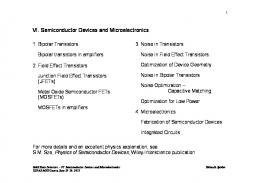
5-3 Simulation Results Two simulation results will be shown , the first is a highly doped pn junction , the second is a MOSFET device.

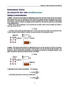
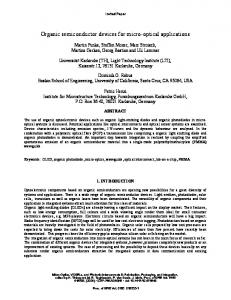
I) PN results The device structure, shown in figure 5-6, is highly doped. The level control function used for controlling the mesh size was chosen depending on the doping gradient. Hence, we will see a high mesh concentration in the depletion region and a fairly course mesh deep inside the P and N regions.

Figure 5-6 PN device

73

Figure 5-7 Triangulation of a PN device The thermal equilibrium case will be considered now. It is known that the built in voltage is

kT 1 1 ( asinh N D  asinh N A ) q

in our case 0.87 V or 33.6 V th . The

next figure shows the scaled potential which agrees well with the analytical result.

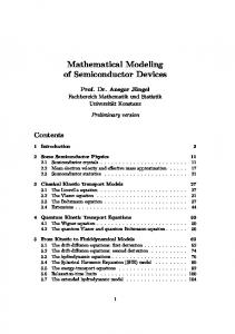
Figure 5-8 Thermal Equilibrium case The electrons concentration, shown in figure 5-9, represents how the electrons density

74

increases in the N- region and approaches N D .

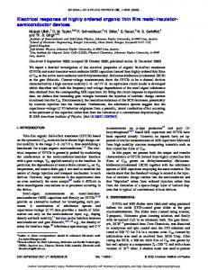
Figure 5-9 Electrons concentration on thermal equilibrium Different bias voltages are applied and the IV - characteristics is plotted .

Figure 5-10 IV-characteristics for the PN junction The red-coloured curve is the analytical value given by:

75

J = J 0 (exp (

V )1) ηV th

5-4

η∈[1 2]

η was found to be 1.5.

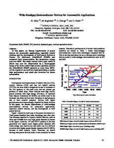
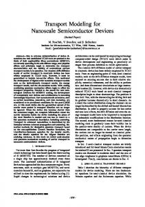
MOSFET results The device structure is shown in figure 5-11. It consists of highly doped drain and source. The MOS is a long channel type, 2.6um. The mesh will be doped heavily in the depletion regions and much heavier in the channel as shown in figure 5-12.

Figure 5-11 A MOSFET Device

Debye Debye

Figure 5-12 Triangulation of a MOSFET A gate voltage of 0.4V ( 18 V th ) is applied and V DS is zero. The potential distribution is shown in figure 5-13

76

Vth

Debye Debye

Figure 5-13 VGS = 0.4V and VDS =0 Different V DS are introduced and the potential distributions are shown V DS =1V th

V DS =5V th Vth

Vth

Debye

Debye

Debye

Debye

Figure 5-14 Different biasing voltages The final IV characteristics curves for different channel lengths are shown in figure 5-15

77

and it is clear how it agrees with the analytical result given by: V 2DS I D =β [(V GS V THN )V DS  ] 2 β I D = (V GS V THN )2 2

V GS >V THN ,

V GS ≥V THN,

V DS