Modelling of the Elasticity Modulus for Rock Using Genetic Expression

Hindawi Publishing Corporation Advances in Materials Science and Engineering Volume 2016, Article ID 2063987, 8 pages http://dx.doi.org/10.1155/2016/2063987

Research Article Modelling of the Elasticity Modulus for Rock Using Genetic Expression Programming Umit Atici Department of Mining Engineering, Engineering Faculty, Nigde University, 51245 Nigde, Turkey Correspondence should be addressed to Umit Atici; [email protected] Received 27 July 2016; Revised 31 August 2016; Accepted 1 September 2016 Academic Editor: Giorgio Pia Copyright © 2016 Umit Atici. This is an open access article distributed under the Creative Commons Attribution License, which permits unrestricted use, distribution, and reproduction in any medium, provided the original work is properly cited. In rock engineering projects, statically determined parameters are more reflective of actual load conditions than dynamic parameters. This study reports a new and efficient approach to the formulation of the static modulus of elasticity 𝐸𝑠 applying gene expression programming (GEP) with nondestructive testing (NDT) methods. The results obtained using GEP are compared with the results of multivariable linear regression analysis (MRA), univariate nonlinear regression analysis (URA), and the dynamic elasticity modulus (𝐸𝑑 ). The GEP model was found to produce the most accurate calculation of 𝐸𝑠 . The proposed approach is a simple, nondestructive, and practical way to determine 𝐸𝑠 for anisotropic and heterogeneous rocks.

1. Introduction Strength and deformation features play an important role in the design of rock structures [1]. The elasticity modulus is an important parameter in understanding stress-strain behaviour and is one of the most mechanical characteristics of rocks in regarding their using area [2]. This parameter is decisive in tunnel project, rock destruction and drilling, slope consistency, pillar configuration, embankments, and many other civil and mining applications [3]. It has been used extensively for the analysis of structural deformations, creep, shrinkage, crack control, and so forth [4–6]. Either static or dynamic various numbers of methods are available for determination of deformation parameters. The static elasticity modulus (𝐸𝑠 ) can be obtained from conventional laboratory procedures, for example, from the incline of tensile test stress-strain diagrams, but as they are generally time consuming and expensive even on a laboratory applications, the number of tests in many projects is limited. On the other hand, the dynamic elasticity modulus (𝐸𝑑 ) can be determined from compression (𝑉𝑝 ) and shear (𝑉𝑠 ) wave velocities, and knowledge of the rock density (𝜌) is based essentially on rapidly applied nondestructive loads; in many cases this requires simple and easy operations.

During the design of rocks inside structures, statically achieved parameters are preferred rather than those obtained by dynamic methods as the statically determined ones are more reflective of real loading situations [1]. The values of elastic constants often disagree with those determined by static laboratory methods. Hence, the true 𝐸𝑠 is usually different from values determined by either static or dynamic methods. According to ASTM-D2845-08 [7], elastic constants are not to be calculated using procedures described in the test method for rocks with pronounced anisotropy. For these reasons, 𝐸𝑑 measurements are not common in rock engineering projects. Most rock materials do not behave in completely linear elastic, homogenous, isotropic mode, and hence there is a difference between 𝐸𝑠 and 𝐸𝑑 . Dynamic test methods therefore supply data that are only meaningful for the designing stage in rock engineering [8]. Because of the advantages of 𝐸𝑑 and the validity of 𝐸𝑠 , many researchers have aimed to predict 𝐸𝑠 from 𝐸𝑑 using multivariable linear regression analysis (MRA). Some of these authors include [9–11]. According to these studies, the 𝐸𝑑 determined is generally higher than 𝐸𝑠 . MRA modelling in particular has been used for some time because it has the advantage of performing easy-to-use regression constants to facilitate estimation of the significance of various input

2 variables and is established by precharacterization of the construction of a model with a limited number of linear or nonlinear equations. Lama and Vutkuri [12] reported that 𝐸𝑑 is greater than 𝐸𝑠 by up to 300%. It must be appreciated that predicting 𝐸𝑠 from 𝐸𝑑 is ultimately an inverse problem. To cope with these limitations and challenges, several alternative soft computing techniques have been used considerably to model human activities in various areas of engineering. Learning from experience and deriving the information is one of the essential properties of soft computing techniques. Artificial neural networks, adaptive neurofuzzy inference systems, and fuzzy logic methods are commonly used in many engineering applications. A major disadvantage of these systems is that they are not able to provide practical prevision equations [4, 13]. To overwhelm the restrictions of these techniques, genetic programming (GP) and its variants, such as linear genetic programming (LGP) and gene expression programming (GEP), have been used in engineering applications in recent years. In civil engineering applications, GP, LGP, and GEP have been applied successfully to behavioural modelling of the elastic modulus of concrete [4, 14]. Engineers in different countries are keen on nondestructive testing (NDT) to assess rock properties. These types of tests are simple to conduct as they need less or no specimen preparation and the test device is also simple [15, 16]. NDT methods, ultrasonic pulse velocity (UPV), and rebound hammer (RN) testers among preferable methods are the most generally used in application to determine rock characteristics. A number of researchers, including [17–20], have studied the relationship between rock properties and NDT. The present study mainly aimed to investigate the use of GEP in predicting 𝐸𝑠 for rock materials. Application of the GP methods pointed out higher amount of nonlinear relationship between experimental and estimated values with high precision and comparatively low error. Because GEP put together the advantages of genetic algorithms (GA) and GP, it has verified to be an effective modelling instrument for solving complex real-world problems, and complex relationships between parameters affecting 𝐸𝑠 can be modelled easily by using a GEP approach [21]. In contrast to dynamic elasticity, there is no definitive formulation for anticipating the 𝐸𝑠 of rock. For this reason, the GEP approach is preferred to build empirical models. To build the model, 𝐸𝑠 results of 317 specimens were used in training, testing, and validation. The data sets were derived from an experimental study performed as part of this project. Three main parameters that clearly influenced 𝐸𝑠 were selected as input variables: compression wave velocity (𝑉𝑝 ), Schmidt rebound hardness (RN), and rock density (𝜌). The results obtained were compared with those of other approaches to demonstrate the superiority and practicality of the proposed approach.

2. Materials and Methods Samples of the rock materials were collected from various locations, mostly in Turkey but also from various other

Advances in Materials Science and Engineering Table 1: Mechanical and physical features of rocks used in experiments. 3

𝜌 (g/cm ) 𝑉𝑝 (km/s) 𝑉𝑠 (km/s) RN 𝑓𝑐 (MPa) 𝐸𝑠 (GPa)

Min 1.91 0.74 0.48 0.5 1.32 0.51

Max 3.24 6.48 5.13 70.6 183 94

Mean 2.65 4.23 2.71 41.44 72.34 31.14

Standard deviation 0.28 1.26 0.99 16.85 39.60 22.68

regions of the world. The rock blocks consisted mainly of marble, limestone, and igneous and magmatic rock. The rock samples used in the research program were received in the form of cylindrical pieces of NX-sized cores. The specimen density (𝜌) was calculated from their dimensions and weights at a temperature of 20 ± 3∘ C. The velocities of compression (𝑉𝑝 ) and shear (𝑉𝑠 ) waves were recorded in cylindrical core samples applying the highfrequency ultrasonic pulse technique proposed by ASTM [7]. The Schmidt hammer rebound (RN) test method is used crustily to examine the strength and quality of rock and hardened concrete. There is a strong relationship between the RN and the uniaxial compressive strength (𝑓𝑐 ) of rock. The RN values of the rock specimens were obtained using an N-type Digi-Schmidt 2000 apparatus according to the procedures described in ASTM C 805 [22]. At least 20 measurements were taken at different points on each mixture sample. Rock’s most important parameter is its compressive strength (𝑓𝑐 ) as it was indicated earlier [3]. The 𝑓𝑐 properties of rocks were determined related with standards proposed by ASTM D7012-14 [23]. At least five core samples from each rock were subjected to strength tests performed by a fully automatic, instrumented, and computer-controlled press machine. For determination of 𝐸𝑠 , full bridged electrical resistance strain gauges were used. Two strain gauge rosettes, consisting of two gauges each, were bonded to the surface of each specimen at two directly opposite points located halfway between the specimen ends for the measurement of axial and circumferential strains, which were recorded at 1s gaps performing a static data logger. The tangential 𝐸𝑠 was calculated according to the stress-strain curves derived. The mechanical and physical properties of the rocks are presented in Table 1.

3. Regression Analysis SPSS packet programming was used for statistical analysis. For modelling, multivariable linear (MRA) and univariate nonlinear regression analysis (URA) were applied. The reason to apply MRA is to detect simultaneously more independent variables that justify variations in the dependent variable. 𝐸𝑠 is considered to be the dependent variable and the rock properties 𝑉𝑝 , 𝑉𝑠 , RN, 𝑓𝑐 , and 𝜌 are independent variables. MRA was performed to detect the relationships among five independent variables thought to be relevant to 𝐸𝑠 .

Advances in Materials Science and Engineering

3

Table 2: Summary statistics for the five models of multivariable linear regression analysis. Model number

𝑅2

Std. error of estimate

1

Independent variables that contribute to model 𝑉𝑝

0.570

14.88615

2

𝑉𝑝 , RN

0.654

13.37531

3

𝑉𝑝 , RN, 𝜌

0.683

12.82088

4

𝑉𝑝 , RN, 𝜌, 𝑓𝑐

0.691

12.67647

Table 3: Regression coefficient values for univariate nonlinear regression analysis. Models Linear Logarithmic Inverse Quadratic Cubic Compound Power S Growth Exponential Logistic

𝜌 0.518 0.494 0.463 0.548 0.547 0.580 0.589 0.588 0.580 0.580 0.580

Independent variable RN 𝑓𝑐 0.356 0.409 0.262 0.373 0.071 0.094 0.356 0.419 0.358 0.421 0.415 0.453 0.530 0.613 0.282 0.299 0.415 0.453 0.415 0.453 0.415 0.453

𝑉𝑝 0.570 0.507 0.350 0.576 0.582 0.667 0.719 0.639 0.667 0.667 0.667

Regression analyses were carried out using SPSS 16 statistical software, which offers a stepwise regression method. Stepwise regression provides insight into which independent variables are significant by identifying good (although not necessarily the best) subset models, resulting in considerably less computing time than would be required to calculate all possible regressions. During the MRA and URA, 5 and 55 different models were created, respectively. Linear, logarithmic, inverse, quadratic, cubic, compound, power, S-curve, growth, exponential, and logistic models were formed and tested individually for nonlinear regression analysis. In these multivariable and univariate models, the highest regression coefficient (𝑅2 ) value is 0.69 for model 4 (Table 2) and 0.72 for the powertype model (Table 3), where 𝑉𝑝 is an independent variable. The results of the multivariable and univariate regression coefficients (𝑅2 ) for these models exist to range within an plausible extent. Because of these results, there is no need to assess the validity of these models further.

4. Gene Expression Programming GEP is a new evolutionary artificial intelligence method developed by Ferreira [24]. It is a strong evolutionary algorithm that includes both simple linear chromosomes of arranged length, similar to those performed in genetic algorithms (GA), and separated structures of different sizes and structures, similar to the parsing trees of genetic programming (GP). Its evaluation system for any type of knowledge

mirrors that of biological evaluation and is encoded as a computer program in linear chromosomes of fixed length. In this method, a mathematical function identified as a chromosome with multiple genes is developed using the data presented to it. Although GEP mainly executes symbolic regression through most of the genetic operators of GA and GP, there are some differences between GA, GP, and GEP. GP represents it as nonlinear essences of different sizes and shapes (parsing trees) while any mathematical expression is adopted as a symbolic string of fixed length (chromosomes) in GA. However, in GEP it is encoded as simple strings of fixed length, which are subsequently expressed as expression trees of different sizes and shapes [25, 26]. One such gene, expression tree (ET), and its algebraic expression can be represented in Figure 1. For more detailed information, the reader is referred to Ferreira [24, 27]: Mathematical Equation: √(𝑎 − 𝑏) (𝑐 + 𝑑).

(1)

4.1. GEP Model. The principle in the development of GEP models was to generate a mathematical function for predicting 𝐸𝑠 using only NDT methods (RN, 𝑉𝑝 ) and 𝜌. When selecting these variables, it has been noted that they are used in the estimation of 𝐸𝑑 , which is provided by well-known methods to determine the deformation characteristics of materials. The widely used parameters in the determination of 𝐸𝑑 are 𝑉𝑝 , 𝑉𝑠 , and 𝜌. Previous researchers have demonstrated that 𝑉𝑝 and 𝑉𝑠 [28, 29] as well as compressive strength and RN [30, 31] are highly correlated. Multicollinearity, a strong correlation between independent variables, might result in problems with the analysis. For example, variables do not contribute sufficiently to the model. Because of multicollinearity and the fact that measurements of 𝑉𝑠 are more difficult than those of 𝑉𝑝 , and because RN is a nondestructive technique that does not damage the sample, 𝐸𝑠 is formulated as a function of 𝑉𝑝 , RN, and 𝜌 values of rocks. The GEP model was developed using data sets of 317 rock specimens obtained from an experimental study. Both the practicing and examination data were randomly selected from these data. The numbers of experimental data sets used for initial practices and testing/validation in this model were 212 and 105, respectively. The parameters used in GEP model development are summarized in Table 4. For GEP formulation, the fitness 𝑓𝑖 of an individual program is measured by 𝐶

𝑡 󵄨 󵄨 𝑓𝑖 = ∑ (𝑀 − 󵄨󵄨󵄨󵄨𝐶𝑖𝑗 − 𝑇𝑗 󵄨󵄨󵄨󵄨) ,

(2)

𝑗=1

where 𝑀 is the range of selection, 𝐶(𝑖, 𝑗) is the value returned by the individual chromosome for performance case 𝑗 (out of 𝐶𝑡 fitness cases), and 𝑇𝑗 is the target value for fitness case 𝑗. If |𝐶(𝑖𝑗) − 𝑇𝑗 | (the precision) is less than or equal to 0.01, then the accuracy is equal to zero, and 𝑓𝑖 = 𝑓max = 𝐶𝑡 𝑀. In this case, 𝑀 = 100 was used; therefore, 𝑓max = 1000. Since the system can find the optimal solution by itself, it can be considered as the advantage of this type of fitness function [24, 32, 33]. Next, the set of terminals “𝑇” and the set of functions “𝐹” used to create the chromosomes are chosen, namely, 𝑇 = {𝑉𝑝 , RN, 𝜌},

4

Advances in Materials Science and Engineering

Q

∗

−

a

+

b

c

Mathematical equation: √(a − b)(c + d)

d

Figure 1: Example of GEP expression tree and mathematical equation.

and four basic arithmetic operators (+, −, ∗, /) and some basic mathematical functions (Sqrt, Cubic Root, 4Rt, Sub3, Exp, 𝑥3 , 1/𝑥, Ln) were used. For choosing the chromosomal tree, that is, the length of the head and the number of genes, the GEP approach model initially used a single gene and two lengths of heads and increased the number of genes and heads, one after another, during each run, while monitoring the training and testing performance of each model. In the present study, after several

trials, to achieve the best results the number of genes and length of heads were found to be 4 and 17, respectively. The sub-ETs (genes) were linked by multiplication. Finally, a combination of all genetic operators (mutation, transposition, and crossover) was utilized as the set of genetic operators. Parameters used for training the GEP approach model are given in Table 1. Chromosome 20 was observed to be the best generation of individuals in predicting 𝐸𝑠 . The definitive formulation of 𝐸𝑠 based on the GEP approach model is given by

} { } { 1 𝐸𝑠 = { } 3 } { √3 4 [ √𝑑2 ∗ 𝑑1 ∗ 𝑐1 ∗ [(𝑐3 /𝑐2 ) − (𝑑0 /𝑐4 ) ]] − Arctan [(𝑑0 − 𝑐2 ) ∗ 𝑐0 ] } { ∗ {[√5 𝑑2 − 𝑑22 ] − [Arctan√ [Arctan (1/𝑑1 )] + [𝑑2 + (𝑑0 − 𝑐1 )] ∗ Ln√4 𝑑1 ]} 5

2 ∗ {𝑑0 − [𝑑1 − [𝑐4 ∗ [𝑑0 − √𝑐 1 ] − [(

(3)

𝑑2 5 − 𝑑0 )]] ∗ [(𝑐3 ∗ 𝑑2 ) − (𝑑0 ∗ 𝑐3 )] ]} 𝑐2

5 } { 1 2 ] ∗ [√ (√2 (𝑑2 ∗ 𝑐2 )) ]} . ∗ {𝑑0 + Tanh [[(𝑐2 ∗ 𝑐1 ) ∗ (𝑐0 − 𝑑2 )] − 𝑑1 ] ∗ [ 3 (𝑑02 ) [ ]} {

The representation tree of the formulation is also shown in Figure 2, where 𝑑0 , 𝑑1 , and 𝑑2 refer to 𝜌, RN, and 𝑉𝑝 , respectively. The constants in the formulation are given in Table 5.

5. Results and Discussion This study is supposed to find out possible the pertinence of GEP, MRA, and URA in predicting the 𝐸𝑠 value of rocks, which has great significance in rock mechanics and foundation engineering. The developed models were compared with 𝐸𝑑 . This part relatively presents the analysis results derived from these approaches and quantitative evaluations of the predictive capabilities of the models.

Of the 317 data sets, 212 were used for training the models and the 105 that were not used in training were used to test the models. To determine the success of the developed models, the regression coefficient (𝑅2 ), root-mean-square error (RMSE), and average absolute percentage error (MAPE) were used as criteria to assess compatibility between the experimental and predicted values. The statistical success of the developed models and 𝐸𝑑 values is shown in Table 6. The 𝑅2 value relating the experimental and predicted data using the GEP model is 0.90, implying that the GEP model has good performance. On the other hand, the 𝑅2 values of the MRA, URA (a power model where 𝑉𝑝 is the independent variable), and 𝐸𝑑 models are 0.68, 0.72, and 0.43, respectively.

Advances in Materials Science and Engineering

5

Sub-ET 1

Inv +

3Rt

− −

∗ c1

4Rt

X3

/ c3

∗ d2

Arctan

c2

∗

c4

d0

d1

c0

−

/ d0

c2

Sub-ET 2 − 5Rt

Arctan

−

5Rt X2

d2

∗

d2

Ln

+

Inv

d2

c1

−

d1 Sub-ET 3

4Rt

+

Arctan

c1

d0

− −

d0 d1

∗ X5

∗ c4

−

− −

− d0

/

Sqrt c1

Sub-ET 4

∗

d2

d0

c3

∗ d2

c2

+

∗

d0

Sqrt

∗ Tanh

Inv

X5

−

X3

Sqrt

∗

∗

d1

∗ ∗ c2

− c1

c0

d0

d0

d2

Figure 2: Expression tree for the GEP model.

d2

c2

d0

c3

6

Advances in Materials Science and Engineering 160

R2 = 0.9001

60

R2 = 0.4301

120 Ed (GPa)

Predicted Es (GPa)

80

40

20

80

40

0 0

20

40 Observed Es (GPa)

60

0

80

0

Figure 3: Measured versus predicted 𝐸𝑠 for data used to train the GEP model. 80

20

40

60

Figure 5: Comparison of static and dynamic elasticity.

Predicted Es (GPa)

Parameter definition

GEP model

Program size Literals Number of generations Arithmetic operators

60

40

Mathematical functions

20

0 10

20

100

Table 4: GEP parameters used for the developed model.

R2 = 0.9114

0

80

Es (GPa)

30 40 50 60 Observed Es (GPa)

70

80

90

Figure 4: Measured versus predicted 𝐸𝑠 for data used to validate the GEP model.

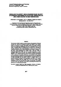
These values are not sufficient for confident validation of these models. The 𝐸𝑠 values predicted from GEP methods for training and testing are compared graphically with their experimental counterparts in Figures 3 and 4, respectively. As can be seen from these figures, there is a close compatibility between real and anticipated values. Figure 5 shows the comparison between 𝐸𝑠 and 𝐸𝑑 values. As can be clearly seen in these figures, there is no relationship between the predicted and observed variables, and the results obtained by these methods are very different from the experimental results (𝑅2 = 0.43). In fact, for 𝐸𝑑 in this study, even negative values are observed. As a result of the evaluation of these results, the GEP model was determined as the best applicable model for predicting 𝐸𝑠 in comparison with MRA and 𝐸𝑑 .

6. Conclusions Findings of the presented study reported a new and efficient approach to the formulation of 𝐸𝑠 using GEP with NDT and

Number of chromosomes Head size Tail size Gene size Number of genes Linking function Mutation rate Inversion rate One-point recombination rate Two-point recombination rate Gene recombination rate Gene transposition rate

95 23 10,024,415 +, −, ∗, / Inv, sgrt, 3Rt, 4Rt, 5Rt, 𝑋2 , 𝑋3 , 𝑋4 , 𝑋5 , arctangent and hyperbolic tangent 20 17 18 53 4 Multiplication 0.00138 0.00546 0.00277 0.00277 0.00277 0.00277

Table 5: Constants in the GEP model. Constant 𝐶0 𝐶1 𝐶2 𝐶3 𝐶4

Sub-ET 1 3.61 11.19 3.07 3.20 −4.00

Sub-ET 2 −4.31 6.00 5.51 5.81 −8.86

Sub-ET 3 7.18 16.88 5.85 −0.58 −0.68

Sub-ET 4 5.91 6.98 10.29 −6.25 5.70

led to compare findings of MRA, URA, and 𝐸𝑑 . The proposed model is empirical, and data for its development were derived from the experimental study conducted. It was shown that the GEP model considerably outperforms compared to other soft computing systems mentioned above. This was supported

Advances in Materials Science and Engineering

7

Table 6: Statistical parameters for predicting 𝐸𝑠 . GEP model Training Validation 𝑅2 0.90 RMSE 7.02 MAPE 5.44

0.91 6.66 4.97

Best MRA model

Best URA model

𝐸𝑑

0.68 12.27 87.96

0.72 46.10 98.49

0.43 26.53 102.56

and proven by statistical fitness criteria used for evaluating the models. The GEP model produced the highest 𝑅2 value (0.90) and lower RMSE and MAPE values (7.02 and 5.44, resp.). GEP is particularly suitable for predicting 𝐸𝑠 values of rocks from anisotropic and heterogeneous materials in terms of calculating nonlinear functional relationships where classical methods cannot be easily performed. Moreover, with the use of GEP, 𝐸𝑠 can be estimated without performing sophisticated and time-consuming laboratory tests. The proposed method is simple, does not damage the sample, and is sufficiently accurate to be recommended for use in practice.

[9]

[10]

[11]

[12]

[13]

[14]

Competing Interests The author declares that there is no conflict of interests regarding the publication of this paper.

References [1] E. A. Eissa and A. Kazi, “Relation between static and dynamic youngs moduli of rocks,” International Journal of Rock Mechanics and Mining Science & Geomechanics Abstracts, vol. 25, no. 6, pp. 479–482, 1988. [2] V. Brotons, R. Tom´as, S. Ivorra, and A. Grediaga, “Relationship between static and dynamic elastic modulus of calcarenite heated at different temperatures: the San Juli´an’s stone,” Bulletin of Engineering Geology and the Environment, vol. 73, no. 3, pp. 791–799, 2014. [3] M. Karakus, M. Kumral, and O. Kilic, “Predicting elastic properties of intact rocks from index tests using multiple regression modelling,” International Journal of Rock Mechanics and Mining Sciences, vol. 42, no. 2, pp. 323–330, 2005. [4] A. M. Bayazidi, G.-G. Wang, H. Bolandi, A. H. Alavi, and A. H. Gandomi, “Multigene genetic programming for estimation of elastic modulus of concrete,” Mathematical Problems in Engineering, vol. 2014, Article ID 474289, 10 pages, 2014. [5] A. H. Gandomi, A. H. Alavi, M. G. Sahab, and P. Arjmandi, “Formulation of elastic modulus of concrete using linear genetic programming,” Journal of Mechanical Science and Technology, vol. 24, no. 6, pp. 1273–1278, 2010. [6] H. A. Mesbah, M. Lachemi, and P.-C. A¨ıtcin, “Determination of elastic properties of high-performance concrete at early ages,” ACI Materials Journal, vol. 99, no. 1, pp. 37–41, 2002. [7] ASTM, “Standard test method for laboratory determination of pulse velocities and ultrasonic elastic constants of rock,” ASTM D2845-08, American Society for Testing and Materials International, West Conshohocken, Pa, USA, 2008. [8] W. L. Heerden, “General relations between static and dynamic moduli of rocks,” International Journal of Rock Mechanics and

[15]

[16]

[17]

[18]

[19]

[20]

[21]

[22]

[23]

Mining Sciences & Geomechanics Abstracts, vol. 24, no. 6, pp. 381–385, 1987. M. S. King, “Static and dynamic elastic properties of rocks from the Canadian shield,” International Journal of Rock Mechanics and Mining Science & Geomechanics Abstracts, vol. 20, no. 5, pp. 237–241, 1983. A. Dziedzic and J. Pini´nska, “The static and dynamic elasticity parameters of laminated silty-clay shales at the simulated depth up to 4 km,” in Proceedings of the ISRM European Regional Symposium on Rock Engineering and Rock Mechanics: Structures in and on Rock Masses (EUROCK ’14), pp. 223–228, May 2014. L. Miranda, L. Cantini, J. Guedes, and A. Costa, “Assessment of mechanical properties of full-scale masonry panels through sonic methods. Comparison with mechanical destructive tests,” Structural Control and Health Monitoring, vol. 23, no. 3, pp. 503– 516, 2016. R. D. Lama and V. S. Vutukuri, Series on Rock and Soil Mechanics Ii Handbook on Mechanical Properties of Rock: Testing Techniques and Results, Trans Tech Clausthal, New York, NY, USA, 1978. A. H. Alavi and A. H. Gandomi, “A robust data mining approach for formulation of geotechnical engineering systems,” Engineering Computations, vol. 28, no. 3, pp. 242–274, 2011. A. H. Gandomi, A. H. Alavi, T. O. Ting, and X. S. Yang, “Intelligent modeling and prediction of elastic modulus of concrete strength via gene expression programming,” in Advances in Swarm Intelligence: 4th International Conference, ICSI 2013, Harbin, China, June 12–15, 2013, Proceedings, Part I, Lecture Notes in Computer Science, pp. 564–571, Springer, Berlin, Germany, 2013. H. Y. Qasrawi, “Concrete strength by combined nondestructive methods simply and reliably predicted,” Cement and Concrete Research, vol. 30, no. 5, pp. 739–746, 2000. S. Kahraman, “Evaluation of simple methods for assessing the uniaxial compressive strength of rock,” International Journal of Rock Mechanics and Mining Sciences, vol. 38, no. 7, pp. 981–994, 2001. E. Yasar and Y. Erdogan, “Correlating sound velocity with the density, compressive strength and Young’s modulus of carbonate rocks,” International Journal of Rock Mechanics and Mining Sciences, vol. 41, no. 5, pp. 871–875, 2004. G. Vasconcelos, P. B. Lourenc¸o, C. A. S. Alves, and J. Pamplona, “Ultrasonic evaluation of the physical and mechanical properties of granites,” Ultrasonics, vol. 48, no. 5, pp. 453–466, 2008. U. Atici, “Prediction of the strength of mineral admixture concrete using multivariable regression analysis and an artificial neural network,” Expert Systems with Applications, vol. 38, no. 8, pp. 9609–9618, 2011. A. Azimian, R. Ajalloeian, and L. Fatehi, “An empirical correlation of uniaxial compressive strength with p-wave velocity and point load strength index on marly rocks using statistical method,” Geotechnical and Geological Engineering, vol. 32, no. 1, pp. 205–214, 2014. H. M. Azamathulla, A. A. Ghani, C. S. Leow, C. K. Chang, and N. A. Zakaria, “Gene-expression programming for the development of a stage-discharge curve of the Pahang River,” Water Resources Management, vol. 25, no. 11, pp. 2901–2916, 2011. ASTM, “Test for rebound number of hardened concrete,” ASTM C 805, American Society for Testing and Materials International, West Conshohocken, Pa, USA, 1997. ASTM D7012-14, Standard Test Methods for Compressive Strength and Elastic Moduli of Intact Rock Core Specimens under

8

[24]

[25]

[26]

[27]

[28]

[29]

[30]

[31]

[32]

[33]

Advances in Materials Science and Engineering Varying States of Stress and Temperatures, American Society for Testing and Materials International, West Conshohocken, Pa, USA, 2014. C. Ferreira, “Gene expression programming: a new adaptive algorithm for solving problems,” Complex Systems, vol. 13, no. 2, pp. 87–129, 2001. A. Cevik, “A new formulation for longitudinally stiffened webs subjected to patch loading,” Journal of Constructional Steel Research, vol. 63, no. 10, pp. 1328–1340, 2007. C. Kayadelen, “Soil liquefaction modeling by genetic expression programming and neuro-fuzzy,” Expert Systems with Applications, vol. 38, no. 4, pp. 4080–4087, 2011. C. Ferreira, Gene-Expression Programming; Mathematical Modeling by an Artificial Intelligence, Springer, Heidelberg, Germany, 2006. H. Soroush and F. Ahmad, “Evaluation of some physical and mechanical properties of rocks using ultrasonic pulse technique and presenting equations between dynamic and static elastic constants,” in Proceedings of the 10th ISRM Congress, International Society for Rock Mechanics, Sandton, South Africa, September 2003. H.-T. Cai, H. Kuo-Chen, X. Jin, C.-Y. Wang, B.-S. Huang, and H.-Y. Yen, “A three-dimensional Vp, Vs, and Vp/Vs crustal structure in Fujian, Southeast China, from active- and passivesource experiments,” Journal of Asian Earth Sciences, vol. 111, pp. 517–527, 2015. N. Yesiloglu-Gultekin, C. Gokceoglu, and E. A. Sezer, “Prediction of uniaxial compressive strength of granitic rocks by various nonlinear tools and comparison of their performances,” International Journal of Rock Mechanics and Mining Sciences, vol. 62, pp. 113–122, 2013. A. Aydin, “ISRM suggested method for determination of the Schmidt hammer rebound hardness: revised version,” in The ISRM Suggested Methods for Rock Characterization, Testing and Monitoring: 2007–2014, pp. 2007–2014, Springer, Berlin, Germany, 2015. I. F. Kara, “Prediction of shear strength of FRP-reinforced concrete beams without stirrups based on genetic programming,” Advances in Engineering Software, vol. 42, no. 6, pp. 295–304, 2011. M. Saridemir, “Effect of specimen size and shape on compressive strength of concrete containing fly ash: application of genetic programming for design,” Materials and Design, vol. 56, pp. 297–304, 2014.

Journal of

Nanotechnology Hindawi Publishing Corporation http://www.hindawi.com

Volume 2014

International Journal of

International Journal of

Corrosion Hindawi Publishing Corporation http://www.hindawi.com

Polymer Science Volume 2014

Hindawi Publishing Corporation http://www.hindawi.com

Volume 2014

Smart Materials Research Hindawi Publishing Corporation http://www.hindawi.com

Journal of

Composites Volume 2014

Hindawi Publishing Corporation http://www.hindawi.com

Volume 2014

Journal of

Metallurgy

BioMed Research International Hindawi Publishing Corporation http://www.hindawi.com

Volume 2014

Nanomaterials

Hindawi Publishing Corporation http://www.hindawi.com

Volume 2014

Submit your manuscripts at http://www.hindawi.com Journal of

Materials Hindawi Publishing Corporation http://www.hindawi.com

Volume 2014

Journal of

Nanoparticles Hindawi Publishing Corporation http://www.hindawi.com

Volume 2014

Nanomaterials Journal of

Advances in

Materials Science and Engineering Hindawi Publishing Corporation http://www.hindawi.com

Volume 2014

Journal of

Hindawi Publishing Corporation http://www.hindawi.com

Volume 2014

Journal of

Nanoscience Hindawi Publishing Corporation http://www.hindawi.com

Scientifica

Hindawi Publishing Corporation http://www.hindawi.com

Volume 2014

Journal of

Coatings Volume 2014

Hindawi Publishing Corporation http://www.hindawi.com

Crystallography Volume 2014

Hindawi Publishing Corporation http://www.hindawi.com

Volume 2014

The Scientific World Journal Hindawi Publishing Corporation http://www.hindawi.com

Volume 2014

Hindawi Publishing Corporation http://www.hindawi.com

Volume 2014

Journal of

Journal of

Textiles

Ceramics Hindawi Publishing Corporation http://www.hindawi.com

International Journal of

Biomaterials

Volume 2014

Hindawi Publishing Corporation http://www.hindawi.com

Volume 2014