Hydrological Sciences-Joumal-des Sciences Hydrologiques, 44(2) April 1999
313
Modelling river discharge for large drainage basins: from lumped to distributed approach V. KRYSANOVA, A. BRONSTERT Potsdam Institute for Climate Impact Research (PIK), PO Box 601203, Telegrafenberg, D-14412 Potsdam, Germany e-mail:
[email protected]
D.-I. MÛLLER-WOHLFEIL National Environmental Research Institute, Vejlsovej 25, DK-8600 Silkeborg, Denmark Abstract The paper presents an upscaled application of the HBV model to the German part of the Elbe drainage basin, and intercomparison of lumped and distributed versions of the model. The objectives of the work were (a) to check the model performance for large-scale basins, and (b) to compare the lumped and distributed versions of the model. Three versions of the HBV model, one lumped and two distributed, were applied first to a number of sub-basins of the Elbe with different hydrological regimes (area > 1000 km 2 ), and then to the whole German part of the basin (area 80 657 km ). The model performed well in all cases. The distributed model versions are more data intensive but enabled better results to be achieved. The perspectives for using the model for large-scale water quality assessment, for climate change impact studies and for coupled land-atmosphere modelling are discussed.
Modélisation du débit des rivières de grands bassins versants: d'une approche agrégée à une approche distribuée Résumé Ce papier présente une application à grande échelle du modèle HBV à la partie allemande du bassin de l'Elbe, ainsi que la comparaison des versions agrégées et distribuées du modèle. Les objectifs de ce travail étaient: (a) de contrôler les performances du modèle pour de grands bassins, et (b) de comparer les versions agrégées et distribuées du modèle. Trois versions du modèle HBV, l'une agrégée et les deux autres distribuées, ont été d'abord appliquées à plusieurs sous-bassins de l'Elbe (superficie > 1000 km ) dont les régimes hydrologiques sont différents, et appliqués ensuite à la totalité de la partie allemande du bassin (superficie 80 657 km ). Les performances du modèle se sont révélées correctes dans tous les cas. Les versions distribuées du modèle nécessitent plus de données mais fournissent de meilleurs résultats. Les perspectives d'utilisation de ce modèle pour l'estimation de la qualité de l'eau sur de vastes étendues, pour des études de l'impact d'une modification climatique et pour la modélisation couplée du système sol-atmosphère sont discutées.
INTRODUCTION Over the last few decades there has been an increasing demand for large-scale hydrological models, particularly as a result of growing awareness of environmental problems and the knowledge that national and transnational measures to improve water resource management and tackle water pollution require adequate assessment tools. Currently there are not many hydrological models that fulfil these requirements (Sivapalan & Blôschl, 1995). Such models should be able to calculate discharge reasonably well for meso-scale and large river basins of area up to 100 000 km2. One important question related to large-scale hydrological modelling concerns how complex the models have to be in order to provide reasonable and stable results. Open for discussion until I October 1999
314
V. Krysanova et al.
Lumped and distributed models According to one of the common classification schemes, hydrological models can be categorized as physically-based or conceptual (Singh, 1995). The physical soundness of the model is usually related to the extent to which the flows of mass, energy and momentum are represented using the basic mathematical equations. Regarding the spatial description of processes, the models may be lumped (all parameters and variables represent average values over the entire area), or distributed (spatial variation of input parameters and variables is accounted for). In addition, a physically-based model should be capable of relating its parameters to physical properties of the modelled area, and usually it has to be fully distributed. Examples of lumped models are the Stanford model (Crawford & Linsley, 1966); the problem-oriented computer language for building Hydrologie Models, HYMO (Williams & Hann, 1972); the flood hydrograph package of the Hydrologie Engineering Center, HEC-1 (Hydrologie Engineering Center, 1981); the model for runoff and streamflow routing in river basins, RORB (Laurenson & Mein, 1983); the tank model (Sugawara, 1984); and the Erosion-Productivity Impact Calculator, EPIC (Williams et al, 1984). The distributed physically-based models are represented by the Système Hydrologique Européen, SHE (Abbot et al., 1986); the Institute of Hydrology Distributed Model, IHDM (Beven et al., 1987); the distributed rainfall-runoff model working with a contour-based method of terrain analysis, THALES (Grayson et al, 1992); and the HILLFLOW model for runoff generation and soil moisture dynamics for hill slopes and small catchments (Bronstert & Plate, 1997). Besides these two classes of models, there is a large number of intermediate tools, which can be related to the semi-distributed class of models. They differ significantly regarding the representation of hydrological processes and the scheme of underlying spatial disaggregation. For example, the Precipitation-Runoff Modelling System, PRMS (Leavesley et al, 1983) subdivides a watershed into Hydrologie Response Units; the SLURP model (original full spelling: Simple Lumped Reservoir Parametric, Kite, 1991) divides a watershed into "Grouped Response Units"; semi-distributed hydrological model, HBV-96 (Lindstrôm et al., 1997) subdivides a basin into subbasins and elevation/vegetation zones: SWAT (Soil and Water Assessment Tool, Arnold et al., 1993) suggests a subdivision into sub-basins or virtual sub-basins based on sub-basin boundaries, land-use and soil data; and SWIM (Soil and Water Integrated Model, Krysanova et al., 1998) applies disaggregation into sub-basins and hydrotopes. The semi-distributed TOPMODEL (Beven & Kirkby, 1979) has physically interprétable parameters and attempts to combine the parametric efficiency of a lumped approach with the link to physical theory. The physical soundness of the hydrological models is critically reviewed in recent literature (Bergstrôm, 1991; Beven, 1989, 1996; Refsgaard & Knudsen, 1996). Beven (1989) argues that "the currently available physically-based distributed models are lumped conceptual models, albeit that they work at the grid scale rather than at the catchment scale." Three features are questioned: (a) the correctness of equations to describe hydrological processes at the grid or hillslope scale; (b) the possibility of estimating model parameters for the grid cells; and (c) the difficulties in testing these models in terms of the internal state variables (which is claimed to be one important advantage over conceptual semi-distributed models). Summarizing all the problems, Beven (1996) suggests that progress will be made in moving "towards simpler, more
Modelling river discharge for large drainage basins: from lumped to distributed approach
315
robust, and more easily calibrated representations of distributed hydrology rather than introducing ever more complexity and ever more parameters to be defined". In other words, application of a disaggregation approach is suggested, in which the hydrological heterogeneity is reflected by the distributed input parameters and the distributed outputs. For example, those precipitation-runoff models that deal with spatially distributed input data are in principle able to provide output information on water availability at specific locations. Hydrological models for large-scale applications The development and use of simulation models in hydrological research has mainly focused on basins smaller than 1000 km2. Many of these models, particularly if detailed and spatially distributed, cannot be simply transferred or extended to larger scales, both for conceptual reasons and due to the lack of operationally available data. Research efforts on large-scale hydrological modelling are needed because water resources management and measures to prevent undesirable impacts are carried out mainly at the regional scale. Examples of large-scale (several tens to several hundred thousand km2) river basin modelling include: (a) application of a water balance model to the Sacramento River to predict monthly and seasonal runoff (Gleick, 1987); (b) modelling of the Amazon and Zambezi discharge with a coupled water balance and water transport model WBM/WTM (Vôrôsmarty et al, 1989; Vôrôsmarty & Moore, 1991); (c) application of SLURP to the Mackenzie River using GCM data (Kite et ai, 1993); (d) modelling water discharge of the River Rhine for climate impact assessment (RHINEFLOW model, Kwadijk & Rotmans, 1995); and (e) regional application of the VIC-2L model to the Weser River in Germany (Lohmann et al, 1998a,b). In general, rather simple approaches are usually used for larger scales. There are two limitations involved here: the computer power and data availability. Generally speaking, the problem under study, the scale and the model complexity are interrelated. There are some examples in the literature, in which increasing complexity of a model does not increase quality of simulations (Refsgaard & Knudsen, 1996). On the other hand, simpler models have lower data demand, less risk of overparametrization and hence better control over the model performance. For largescale hydrological studies semi-distributed approaches seem to be best suited as they avoid an increase in the number of parameters with area, while preserving the underlying conceptual information about the spatially-distributed parameters used for the hydrological response categories defined. Bergstrôm (1991) defined the following strategy in hydrological modelling: "only modifications that significantly improve the results are accepted". How can this strategy be realized in large-scale hydrological modelling? Our task, which seems to be an important and timely issue, was to compare three variants of a conceptual model, differing in their levels of complexity. Approach and objectives Among the models that have been applied operationally at larger scales, the conceptual semi-distributed HBV model (Bergstrôm, 1992; Lindstrôm et al, 1997) has been proven to be a rather robust tool for the assessment of the basin-scale runoff dynamics in various
316
V. Krysanova et al.
parts of the world (Bergstrôm, 1995; Zhang & Lindstrôm, 1996). The model was developed at the Swedish Meteorological and Hydrological Institute (SMHI) for runoff simulation and hydrological forecasting. It can be characterized as a semi-distributed conceptual model, consisting of three main routines: (a) snow accumulation and snowmelt, (b) soil moisture accounting, and (c) runoff response and river routing. The number of parameters to be adapted to the site conditions is kept small: two parameters are responsible for the snow routine (the degree-day snowmelt factor, SM, and the threshold temperature for snowmelt, 77); three parameters for the soil moisture routine (the maximum soil moisture storage, FC, the value of soil moisture above which évapotranspiration reaches its potential level, LP, and the control parameter defining the nonlinear relationship between the runoff coefficient and soil moisture, BETA); and five parameters for the runoff response (three recession coefficients K2, K\, K0, the unsaturated storage threshold, UZL, and the percolation rate, PERC). The potential évapotranspiration can either be given as monthly values, and then corrected for altitude, or calculated using a simple temperature index method. The actual évapotranspiration is calculated, taking into account soil water storage and LP. Lakes are assumed to evaporate at potential rate, and the net lake precipitation and a part of the catchment runoff are routed through the lake. The advantages of the HBV model are that (a) it covers most of the important runoff generating processes by quite simple and robust structures and does not require too extensive input data, (b) it accounts for topographic conditions by defining elevation zones within a basin or sub-basins, and (c) the model was successfully tested in different conditions in more than 40 countries. The known applications deal mainly with basins not exceeding 5000 km2, while a larger basin with an area of 16 576 km2 has been investigated in one case (Bhatia et al., 1984), and recently an overall water balance of the Baltic Sea drainage basin was simulated (Bergstrôm et al., 1998) in the framework of the BALTEX (Baltic Sea Experiment) research program. The lack of land cover representation and some other inconsistencies led to the further development and modification of the model, although the basic modelling concept has remained unchanged (Bergstrôm, 1995). Recently, two distributed versions of the model have been developed as described below. The suitability of the model for the assessment of the hydrological dynamics of large river systems in Europe was investigated within this study, performed for the German part of the Elbe drainage basin. A nested modelling procedure was applied, starting from smaller basins. The objectives of the work were: - to check the model performance for large-scale hydrological modelling, and - to compare the model performance and data needs of the lumped and distributed model versions. In addition, the possibilities of using the model for large-scale water quality assessment and for climate change studies are discussed. METHOD AND DATA Modelling tools Three different model versions were applied in the study: (a) the Nordic HBV model obtained from Norway (N. R. Saelthun, personal
Modelling river discharge for large drainage basins: from lumped to distributed approach
317
communication), (b) HBV-96, being the current PC version of the Swedish Meteorological and Hydrological Institute (SMHI, 1997), and (c) HBV-D, a new UNIX-based distributed version developed at PIK, Potsdam, based on the Nordic HBV model. The Nordic HBV can be characterized as a lumped or semi-distributed model, which allows the basin to be subdivided into 10 elevation zones, and every elevation zone into two vegetation zones, while both HBV-96 and HBV-D enable the basin under study to be discretized into a number of sub-basins first, and then every subbasin into elevation and vegetation zones. Later the term "lumped" will be used in relation to the application of the Nordic HBV. The HBV-D has certain features which are different from the HBV-96: (a) there is no limit on the number of sub-basins and climate/precipitation stations for basins up to 100 000 km2; (b) three runoff components can be obtained as an output (instead of two in HBV-96); and (c) an interface routine to the GRASS (Geographic Resources Analysis Support System) GIS is provided, which extracts necessary spatial parameters from a digital elevation model (DEM), a land-use map and a soil map. Study area All the basins under study (Table 1 ) belong to the German part of the Elbe drainage basin (approximately two-thirds of the whole basin area, = 96 000 km2) (Fig. 1). The River Elbe (length: 1092 km) is one of the longest rivers in Europe, with a drainage basin of 148 268 km2 and 24.9 x 10⁶ inhabitants. About one-third of the drainage area belongs to the Czech Republic. Since large parts of the river systems are located in regions of not more than 1500 m elevation, the river discharge is characterized by winter and spring high water periods. Tphe upper, mainly Czech part of the river is Table 1 Spatial disaggregation, input data, the model version and the corresponding efficiency of simulation for case study basins. Basin, Gauge
Area (km2)
No. of subbasins 80.657 1
Number of elevation/vegetation zones 10/20
Number of climate/precipitation stations 25/0
Elbe, Neu Darchau 3/23 Zschopau, 1.574 1 10/20 Lichtenwalde 4/72 Mulde, 6.171 5 50/100 Bad Diiben WeiBe Elster, 2.479 1 10/20 3/50 Zeitz 30/60 3/50 WeiBe Elster, 2.479 3 Zeitz Unstrut, 6.217 4 40/80 4/68 Laucha 170/340 10/279 Saale, Calbe- 23.687 17 Grizehne 25/663 Elbe, 80.657 44 440 / 880 Neu Darchau * two values correspond to several 4- or 5-year periods.
Model version applied Nordic HBV
Efficiency of simulation (R2) 0.76
HBV-96 HBV-D HBV-96, HBV-D Nordic HBV
0.77, 0.82* 0.81 0.86, 0.87, 0.88*, 0.82 0.78
HBV-D
0.83
HBV-D
0.81
HBV-D
0.77
HBV-D
0.86
318
V. Krysanova et al.
Fig. 1 The German part of the Elbe drainage basin and its five sub-basins used as case studies.
dominated by weirs and dams, whereas the middle part can be considered as a seminatural river system. Its final 142 km are affected by tidal processes. The combination of the natural factors with river management actions have caused a depletion of lowlevel water tables in the lower parts of the river during recent decades. Compared to the discharge behaviour of the Rhine valley, storages of glacial snow packages which act as buffers against both flood discharge and low flow are absent in the upper parts of the Elbe basin due to the lack of high mountain regions in the drainage area. The long-term mean annual precipitation in the drainage basin is 659 mm. The long-term mean discharge of the river Elbe at Neu Darchau is 716 m3 s"1 at the mouth, and the specific discharge is 5.42 1 s"1 km"2, which corresponds to the mean annual runoff of 22.58 x 10⁹ m3 or 171.1 mm (=26% of the annual precipitation). Agriculture areas, which cover about 56% of the total area of the drainage basin, represent one of the most important sources of pollution. The Elbe and its tributaries are intensively used for freshwater supply (drinking water, irrigation water and industrial process water). Many large Czech and German nature reserves are situated in the Elbe drainage area. The UNESCO biosphere reserve "Middle Elbe" has been established to protect one of the largest continuous alluvial forests in Central Europe.
Modelling river discharge for large drainage basins: from lumped to distributed approach
319
Data The Neu Darchau gauging station (Fig. 1), which is situated at a distance of 192 km from the North Sea, was chosen for modelling, because it is practically uninfluenced by tidal effects. All input data were prepared for the middle part of the basin (80 657 km2), from the Schôna gauging station, located on the border between Germany and the Czech Republic, down to the Neu Darchau gauging station. The stream length between Schôna and Neu Darchau is 533 km. A digital elevation model with 1 km resolution and the national land-use map for Germany were used to derive necessary input data. A sub-basin map was created, delineating 44 sub-basins within the Elbe drainage basin with corresponding gauging stations (Fig. 2). The criterion for choosing the gauging stations was that the corresponding drainage area should be larger than 800 km2 (only four sub-basins are smaller). The created sub-basin map is based on the existing sub-basin map of the German Federal Agency of the Environment (Umwelt Bundesamt, UBA) and a number of sub-basin maps created by means of the GRASS GIS (program r. watershed) with different threshold values from 1 x 1km DEM. These 44 sub-basins were used for the distributed modelling of the Elbe basin, and some of them represent smaller case study basins. The number of sub-basins in each case study is indicated in Table 1.
Fig. 2 The German part of the Elbe drainage basin subdivided into 44 sub-basins and the corresponding gauging stations (the sub-basins of the Mulde and the Unstrut are numbered).
320
V. Krysanova et al.
In addition, the soil map BÛK-1000 obtained from the German Federal Institute for Geosciences and Natural Resources (Bundesanstalt fur Geowissenschaften und Rohstoffe, BGR), Hannover, was used for initial estimation of the maximum soil moisture for sub-basins, FC. It was estimated for the upper 1 m soil layer for every soil series, and then averaged for the sub-basins using GRASS. The values for sub-basins are between 220 and 391mm. Climate data (temperature and precipitation) from 25 climate stations located in the Elbe basin were used in the study. In addition, daily precipitation data from 663 precipitation stations in the area were used for the distributed modelling of the Elbe basin and for all five smaller basins (Table 1). In the model applications the climate input data were adjusted for elevation zones. Potential évapotranspiration rates were pre-processed as regionally-specific monthly values (S. Grossman, PIK, personal communication). Based on the DEM, the drainage area of a basin (lumped applications) or every sub-basin (distributed applications) was subdivided into ten equal-area elevation zones. The corresponding hypsographic curves (altitude-area) for the Middle Elbe, Mulde and Unstrut (the latter two with sub-basins) are shown in Fig. 3. About 70% of the area is represented by lowlands with altitudes lower than 200 m. The land-use map was reclassified into four classes: (a) agriculture + grassland, (b) forest, (c) lakes, and (d) urban and other areas, since only two types of vegetation plus lakes are allowed in all the model versions used. There are eight sub-basins without lakes, 23 sub-basins have less than 1% area covered by lakes, eight sub-basins have between 1 and 2 %, and five sub-basins (in the lowland part) have more than 3% area covered by lakes. Arable land was therefore combined with natural grassland and pastures in a single class, and all kind of forests were also considered as one class. After that the areas of the two dominating vegetation types were derived for every elevation zone. All vegetation types have specific parameters for interception storage, correction on temperature index, coefficients of variation of snow distribution, adjustment of maximum soil moisture content, etc. Modelling procedure The lumped Nordic HBV was applied for the WeiBe Elster basin and for the Elbe basin. Then HBV-96 and HBV-D were tested in parallel in application to two nested watersheds of the Elbe in order to compare their results: one of them, Zschopau, was not subdivided into sub-basins, and the second, Mulde, was subdivided into five subbasins. After that, HBV-D was applied to three more basins within the Elbe drainage area: the WeiBe Elster, the Unstrut, and the Saale, in order to check the model's performance for different conditions (soils, topography) and for larger basins. Finally, HBV-D was applied to the Middle Elbe subdivided into 44 sub-basins with the purpose of comparing the distributed and lumped model versions. An overview of the various case studies and data used is given in Table 1. Simulations were performed for the period 1981-1989 (for the Mulde basin: 1981— 1995), with the first three years being considered as a calibration period. The following parameters were used for calibration: three recession coefficients K2, K\ and Ko, the threshold, UZL, the percolation rate, PERC, the threshold temperature for snowmelt, TT, and the maximum soil moisture storage, FC (except for the distributed Elbe
Modelling river discharge for large drainage basins: from lumped to distributed approach
321
1200
-4- MuUe 1000
fit
-*- Unstrut -•- Elbe (0.)
800
d
600
£ 400
—*-
200
^A^^~~^~
20
1200
(a)
1
0
l
40
i
l
t
100%
60
-
-•-1 -i- 2
1000 800 ai ce
-
^t/
-••3
-*- 4 600
-¥•5
E 400 200
"if 1
1
20
1
1
40
i
i
i
60
i
i
'
(b)
100%
Fig. 3 Hypsographic curves (a) for the Elbe (German part), Mulde and Unstrut basins, (b) for five sub-basins of the Mulde, and (c) for five sub-basins of the Unstrut.
application), and the parameters SM, LP and BETA. The Nash & Sutcliffe (1970) efficiency R2 was used as a criterion of fit. Calibration of parameters in application to the Middle Elbe was performed only for the lumped version of the model (years 1985-1988). In order to keep the degree of freedom small, it was decided to use only one set of recession coefficients for all subbasins as basin-specific parameters for the distributed version. In principle, at a more refined stage of modelling, they can vary between sub-catchments, in the case that the model also has to be tested internally for sub-basins. Also, the maximum soil moisture storage parameters were not calibrated for sub-basins in this case, but the initially estimated average values for sub-basins were used. This was done for two reasons:
322
V. Krysanova et al.
(a) to keep the degrees of freedom small, and (b) to enable better comparison of the lumped and distributed model versions. The hydrological modelling of the upper Czech part of the basin was excluded, because meteorological and catchment specific data were not available. Instead, the water discharge at the Schôna gauge was taken as discharge input into the model region. The routing of this input discharge to the catchment outlet at Neu Darchau was performed using two different methods: in the lumped modelling a simple translation approach (lag-time of 7 days) was applied; in the distributed Elbe modelling the measured discharge at Schôna was routed to Neu Darchau by applying a unithydrograph-type function, which routes a given discharge by attributing a translation time and a retention feature. The same procedure was used for routing discharges from sub-basins to the basin outlet. The translation and retention parameters were estimated by applying simple assumptions on flow velocity, and using data on distance to the outlet and river slope.
RESULTS River discharge The model performed rather well in all case studies. The most sensitive model parameters were the recession coefficients (they have to be decreased for the Elbe), the threshold, UZL and the percolation rate, PERC (which have to be increased). The model was practically insensitive to the changes of SM, LP, and BETA. After the calibration, the efficiency criterion R2 reached 0.75 for the calibration period, and 0.76 for the whole period. The small difference of the model efficiency for the calibration and validation periods is an indication of the model robustness. A more detailed description of this application and the results can be found in Krysanova & MiillerWohlfeil (1997). In the next application (Zschopau and Mulde) the performances of HBV-96 and HBV-D model versions were compared. These basins are located in a more mountainous part of the Elbe drainage area, and the recession coefficient had to be increased in comparison with those used for the whole Middle Elbe. The results were similar for the both models (annual efficiency R2 varied from 0.77 to 0.88). The resulting efficiency for three five-year periods 1981-1985 1986-1990, and 1991-1995 for the Mulde was quite stable: R2 = 0.86, 0.88 and 0.87, respectively. The simulated and observed hydrographs for the Mulde at Bad Diiben are presented in Fig. 4. Another set of recession coefficients (similar to that of the Elbe) was found for the Unstrut basin, which has different topography (Fig. 3) and a different hydrological regime than the Mulde. Namely, the mean specific discharge values for the Unstrut gauges Laucha, Oldisleben and Nâgelstedt (2.9, 2.4 and 3.4 1 s 4 km 2 , respectively) are much lower than the values for the Mulde and its tributary gauges Bad Diiben, Erlln, Wechselburg, Zschopau and Borstendorf (5.9, 6.4, 8.8, 8.9 and 9.3 1 s"1 km 2 , respectively). Finally, in the distributed modelling for the Middle Elbe using HBV-D, the efficiency achieved was 7?2 = 0.86, with the same recession parameters as in the lumped application. The parameters used are presented in Table 2. The low flow was
Modelling river discharge for large drainage basins: from lumped to distributed approach
SS co