Bennett, K. P. and Campbell, C. (2000), âSupport vector machines: Hype or Hallelujah?â, Newsletter of the ACM Special Interest Group on Knowledge Discovery ...
Algorithms for Partial Discharge Diagnostics Applied to Aircraft Wiring Weizhong Yan, Kai F. Goebel, Nicole Evers GE Global Research Center Niskayuna, NY 12309 {yan, goebelk, evers} @ crd.ge.com
Abstract This paper describes techniques employed for partial discharge (PD) diagnostics of aircraft wiring. Specifically, we present the algorithmic design choices made in the design of partial discharge diagnostic systems. These choices affect preprocessing, feature extraction, feature selection and classification of the PD data. Data were obtained from lab experiments simulating an on-ground de-energized design where the voltage applied to the wiring under investigation was raised to corona inception voltage. The resulting partial discharges differ in their quality depending on whether they were obtained from undamaged wiring or partially damaged wire. In the case of damaged wire we investigate different levels of damage to the insulation, and in particular different levels of chafing. The partial discharges in their raw form may not necessarily allow the separation between the different wiring conditions (damaged or undamaged). However, we illustrate how separation between damaged and undamaged wires can be accomplished with the use of a set of features that have been carefully selected from a large pool of feature candidates extracted from PD measurements. Keywords: Partial discharge; diagnosis; aircraft wiring; feature selection; classification
1. Introduction Wiring is a critical component in an aircraft. If not carefully monitored, wiring in an aging aircraft can cause serious problems. Aircraft wiring integrity and safety related issues have received a great deal of interest after major accidents (e.g., the Swissair 111 and TWA 800 accidents) in which faulty wiring was considered to be the culprit. For weight reduction, aircraft wiring insulation is much thinner than insulation found in building wiring. The insulation deteriorates with age due to changes in chemical composition; vibration during flights; large temperature, humidity, and altitude changes; and exposure to agents such as dust, salt, moisture and cleaning chemicals. In addition, insulation is also exposed to other mechanical stresses during maintenance that may escalate the degree of damage or crate additional defects. The aforementioned effects will degrade the insulation, causing faults such as cracks, delaminating, and chafes. These insulation defects can cause arcing between wires or surrounding metals. Humidity together with salt and dust depositions can make the arc creation even more probable. Major rewiring programs for particular platforms are currently being used to remove extremely problematic insulation such as kapton. This is a time consuming and costly task and only temporarily evades the problem. As the replacement wiring ages, similar problems may arise and without proper monitoring, serious accidents may again occur.
The main method of detection of aircraft wiring defects is still primarily performed by maintenance personnel via visual inspection. This manual inspection is a slow process and its reliability is not considered satisfactory. Furthermore, as it requires twisting the wiring in order to check chafing, this visual inspection can cause more problems than it can identify. Time Domain Reflectometry (TDR) and Frequency Domain Reflectometry (FDR) are also used in some cases for wiring defect detection. However, these methods have only been proven to detect some faults after they have occurred and their sensitivity to detect impending failures such as partial chafes in the insulation remains to be substantiated. These issues have motivated researchers to search for new solutions. Exploring partial discharges (PDs) for diagnosing aircraft wiring faults is one of the research directions. Partial discharges are a local, partial breakdown event that occurs for example, on the surface or inside insulation of electrical products due to possibly minute defects in insulation structure. These minute defects may be the result of the manufacturing process and/or the result of aging and mechanical damage of the products. While normal (healthy) condition of insulation gives a baseline level of partial discharge activities, increase of partial discharge activities indicates insulation degradation or faults. Using partial discharge activities for diagnosing insulation defects/faults is generally known as “PD diagnosis” [Gulski (1995)]. PD diagnosis has been successful in evaluating the integrity of high voltage insulation systems, such as generators, transformers, and capacitors. Using PD for diagnosing aircraft wiring defects, however, has not been done in real-world applications and carries great challenges. The primary challenge comes from the fact that only very low level of voltage is allowed to apply to aircraft wires, which results in PD signals almost indistinguishable from noise. GE has been engaged in a multiple-generation initiative project funded by ONR, focusing on development of PD diagnostic systems for aircraft wiring diagnosis. This paper reports on some of the progress made on the initial design of an on-ground, de-energized prototype system. The focus of this paper is on the development of diagnostic algorithms, more specifically, on the strategies of improving classification accuracy and reliability of PD diagnostic systems for aircraft wiring fault diagnosis. The rest of the paper is organized as follows. Section 2 briefly describes the experimental tests for generating PD measurement data that are necessary for the design of PD diagnostic systems. Section 3 presents our strategies on feature extraction and feature selection. Section 4 gives the details for the design of the classifier. Some preliminary results are summarized in Section 5. Section 6 concludes the paper.
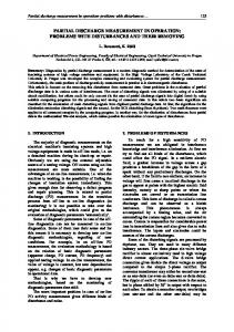
2. Experimental test for partial discharge measurements In order to obtain data examples necessary for designing a PD diagnostic system, laboratory experimental tests are used for generating partial discharges and recording PD measurements. The schematic of the test setup is shown in Figure 1. Damage to wiring insulation generally takes two forms: material degradation due to aging or thermal/electrical environment, and chafing that may occur during maintenance and mechanical abrasion during operation-induced vibration. The lab tests conducted in this paper focus on the latter, i.e., wire chafes. For classifier design purpose, two wiring conditions are tested. One is for normal condition wires and another for wires with artificial chafing. Two different ways are considered in producing artificial defects. The first type represents defects occurring in twisted pair wires. To simulating this, a small piece
of the upper insulation layer was removed from one or both wires in the twisted pair. Samples for this type of defect were prepared from two aircraft grade wires, types M22759/90-22-95 and M22759/81-2252. The second type of defect simulated a chafed wire touching the shielding of the cable bundle or a metal part of the aircraft. The wire was chafed in a short length and a piece of tinned copper wire was twisted around the chafed area. The tinned copper wire was also pressed into the chafed section in order to touch the remaining insulation layer. Such samples were prepared from three aircraft grade wires, types M22759/90-22-95, M22759/81-22-52 and M81044/6-22-9.
Figure 1: PD measurement setup
Unlike most conventional PD measurement systems where only magnitudes and location of PD pulses are recorded, this setup records and stores full PD waveforms and AC waveforms as well with a sampling rate of up to 4.0 GS/s, which allows for a more thorough/advanced analysis of the signals and for extracting more pulse characteristics as well. PD pulses are continuously collected for at least one full AC cycle to obtain complete phase data that aids in defect recognition. For each individual PD pulse, 1500 sampling points are taken. Figure 2 shows a typical PD pulse acquired from the wiring samples. Temperature and humidity of the test chamber are also recorded.
Figure 2: Typical PD pulse
A total of nine wire samples are tested with maximum of 10 repetitions for each sample. After data cleansing (including the removal of noise and incomplete data sets), 596 PD sequences are used for designing the PD diagnostic system. Out of the 596 PD sequences, 225 are for normal wires and 371 for chafed ones.
To study the effects of changing environmental conditions on PD diagnosis for aircraft wiring, the tests are performed under different environmental conditions (pressure and humidity).
3. Feature extraction and selection PD diagnosis is a typical classification problem, that is, to classify measured PD activities into the underlying insulation defects or other causes that generate the PDs. Like in any diagnostic/classification systems, the key to an accurate and reliable PD diagnosis is a set of high quality features/attributes. For PD diagnosis, these features should represent/capture the characteristics of PD signals. More importantly, these features must posses strong discriminant power so that the classifier designed based on those features gives desired performance. Since PD is inherently a stochastic process, namely, the occurrence of PD very much depends on many factors, such as temperature, pressure, applied voltage, and the test duration [Gulski (1995)], and since PD signals contain noise and interference, PD measurements/signals corresponding to different insulation conditions are almost indistinguishable, i.e., PD diagnosis is a complex classification problem. Thus finding a set of high quality features that give accurate and reliable classification is a critical step in the design of PD diagnostic systems. Several feature extraction methods have been proposed for deriving features/fingerprints from PD signals/measurements. However, none of those feature extraction methods have been proved to be effective for all problems. In fact, effectiveness of features from those individual feature extraction methods on classification is highly problem-dependent. That is, features extracted using one method may perform very well for one problem, but may perform poorly for others. Therefore, in design of PD diagnosis systems, finding a method that can identify optimal features for a given problem is still full of challenges [Yan & Goebel (2005)].
Optimal feature set
Feature extraction Method 1
…
Method 2
…
PD measurements
Feature selection
Method n
Initial feature pool
Figure 3: Overall process of finding feature scheme In this paper, we propose a so-called “overproduce and selection” scheme in finding salient features. By collectively utilizing a plurality of feature extraction methods, our scheme can systematically find salient features and guarantees the selected features to be near optimal in terms of PD classification performance. Our approach has two functional components, namely, feature extraction and feature selection. During feature extraction, features are extracted using feature extraction methods from different domains without discerning which method is the best. Then feature selection is tasked to find the optimal subset of features out of all features extracted. Figure 3 illustrates the overall structure of our scheme for finding features for
PD diagnosis. Detailed descriptions of the two components (feature extraction and feature selection) are given in the two subsequent subsections. 3.1. Feature extraction For extracting features from the PD measurements, in this study we used five different methods that have been explored by others for various applications. Following is a brief description of each of the five feature extraction methods. A) Features from statistical analysis of phase-resolved PD patterns. Phase-resolved PD pattern analysis is the most commonly used method for feature extraction in PD diagnosis. Given a sequence of PD pulses and the recorded voltage phase angles at corresponding pulse peaks, a 3D PD pattern is generated, where the number of pulses (pulse count) is plotted as a function of magnitude and phase of the PD pulses. A typical 3D PD pattern is shown in Figure 4. 3D PD patterns are a good representation/summary of all PD pulses recorded within a specified time window and should show different characteristics for different PD activities, thus different PD sources. For the convenience of statistical analysis, the 3D patterns are decomposed into two 2D distributions by projecting it into the two axes - phase and magnitude. Statistical analysis is performed separately for those two distributions. Also, statistical analysis is performed separately for phase angles from 0 ° to 180° (“positive” PDs), for phase angles from 180° to 360° (“negative” PDs), and on the difference between positive and negative PDs. For each of the distributions, two types of statistics, namely amplitude statistics and shape statistics, are calculated. The statistical descriptors are mean, standard deviation, skewness and kurtosis. In addition, overall maximum magnitudes of positive and negative PDs and correlation between positive and negative PD patterns are also calculated as features. The statistical analysis of phase-resolved PD patterns yields 53 different features.
Figure 4: An example of 3D PD patterns
B) Features from PD height distribution analysis. Heights (peaks) of a sequence of PD pulses can be represented in a histogram that shows number of pulses as a function of their magnitude. According to Cacciari et al. (2002), PD pulse height distribution tends to fit well with the two-parameter Weibull function defined as: F (q) = 1 − exp(−(q α ) β ) , where q is the pulse height, α and β are the scale and shape parameters of the Weibull function. Cacciari et al. have found that the scale and shape (especially shape) parameters differ with different PD sources, thus can be used as features for PD identification or classification.
C) Features from “classification map”. PD pulses are different in wave shape depending on the location and nature of the underlying defect that generates PD. One way to capture the different wave shapes is to use so-called “equivalent time-length”, T 2 , and “equivalent bandwidth”, W 2 [Contin et al. (2000)]. In the T 2 − W 2 plane (also called the “classification map” by [Contin et al. (2000)]), each PD pulse is presented as a point and each sequence of PD pulses, which are similar in shape, fall into a well-defined area (cluster) in the T 2 − W 2 plane. The location and shape of the clusters in the T 2 − W 2 plane differ corresponding to different PD sources [Contin et al. (2000 & 2002)]. In this paper, characteristics of the clusters are extracted through statistical analysis and used as features for classification purpose. The features extracted from “classification map” include overall mean, means and standard deviations in both st th T 2 and W 2 directions, respectively, 1 through 4 orders of moments of distributions in both T 2 and W 2 st directions, respectively, direction of the 1 eigenvector of the cluster, and ratio of the first two eigenvalues of the cluster. This yields a total of 15 features from “classification map”. D) Features from spectrum analysis. Frequency spectrum of a PD pulse indicates frequency components of the PD pulse. Thus the shape or distribution of frequency spectra should be correlated with different PD sources. In this paper, the first 3 frequencies corresponding to the highest three magnitudes, the three highest magnitudes themselves, the difference between the three frequencies, and the difference between the three magnitudes are used as features. The total number of features extracted by spectrum analysis is 10. E) Features from raw PD signals. They are the maximum and minimum peaks of PD pulses, mean and standard deviation of peaks of PD pulses, inception voltage, and PD rate, which add 6 more features into the feature pool. The five feature extraction methods yield 86 features in total. Including the temperature and humidity measurements, we have 88 features in the initial feature pool prior to feature selection. Before performing feature selection, a correlation analysis of the 88 extracted features is conducted. Figure 5 displays the heat map representation of correlation coefficients, where each entry represents correlation coefficients between a pair of features. The lighter the field is, the higher the correlation between the feature pair will be. It can be seen that not only do features from one extraction method correlate highly with those from other feature extraction methods, but also there exists fairly high degree of correlation among features within one feature extraction method.
Figure 5: feature-feature correlation coefficients heat map
Figure 6 shows correlation coefficients between each individual feature and the class labels. Features with low feature-class correlation coefficients have low predicting power, thus they are possibly the irrelevant features.
Figure 6: Feature – class correlation (Note: Feature Nos. 1 thru 53 are from Method A, feature Nos. 54 & 55 from Method B, feature Nos. 56 thru 70 from Method C, feature Nos. 71 thru 80 from Method D, and feature Nos. 81 thru 86 from Method E)
3.2. Feature selection Feature selection is a process of choosing a small subset of features out of a given set of candidate features. Feature selection is an important and indispensable step in classifier design for achieving high classification performance. Feature selection has been widely used in various fields, such as pattern recognition, machine learning, and data mining. Dash and Liu (1997) have carried out a comprehensive overview of feature selection techniques. Broadly speaking, feature selection methods can be categorized into filter (also called openloop) methods and wrapper (closed-loop) methods [Langley (1994), Kohavi et al. (1997)]. The filter approach selects features as a result of preprocessing based on properties of the data itself, independently of the learning algorithm. The wrapper approach, on the other hand, uses the learning algorithm as part of the evaluation. Typically, the wrapper approach gives more accurate results, but is also computationally more expensive. There are a variety of feature selection methods available. In this study, GA-based wrapper feature selection is chosen because it provides (near) optimal solutions. Genetic algorithms (GA) are a derivative-free, stochastic optimization method based loosely on the concepts of natural selection and evolutionary processes, which is well suitable for feature selection. GAbased feature selection was first introduced by Siedlecki & Sklansky in 1989. Since then, GA-based feature selection has been actively studied by numerous researchers, for example, Yang and Honavar (1998). In GA-based feature selection, a feature set is represented as a binary vector, where each bit is associated with a feature. A value of 1 at the ith bit means the ith feature is included into the feature set while a value of 0 at the ith bit means the ith feature is not included. In each iteration (generation) of the algorithm, a fixed number (population) of possible solutions are generated in a stochastic fashion. Each of the possible solutions is evaluated and modified following the defined genetic operators. Figure 7 illustrates the concept of GA-based feature selection process
The Genetic Algorithm Optimization Toolbox [Houck et al. (1995)] is used as GA engine. The fitness function used in GA is the evaluation accuracy of the SVM classifier (that is to be described in details in the next section). The GA-based feature selection used here belongs to a “wrapper approach”. Initial population f1 f2 f3 f4
……
0 1 1 0
…
0 1 0
1 1 1 0
…
1 1 0
1 1 1 0
… … …
0 1 1
0 1 1 1 1 1 1 0
New population
fn
Evaluation reproduction modification
0 1 1 1 1 0
f1 f2 f3 f4
……
0 1 1 0
…
f1 f2 f3 f4
……
1 0 1 0
…
0 1 0
0 1 1 0
…
1 1 0
1 1 1 0
… … …
0 0 0
0 0 1 1 1 1 1 0
fn
0 1 0 1 1 0
fn
0 1 0
Feature 2 is included Feature 1 is not included
Figure 7: GA-based feature selection
The GA parameters are: normalized geometric selection with the probability of selecting the best being 8%; simple single-point crossover; and binary mutation with probability of 5%. The population size is 50 and the number of generations is 10. By performing the GA-based wrapper feature selection on the 88 features extracted in the previous subsection, 19 features are selected as the optimal feature set. The 19 features are marked as stars in Figure 6. As can be seen in Figure 6, the 19 selected features are from different feature extraction methods, which indicate the importance of collective utilization of different feature extraction methods. Also, the selected features are not necessarily exclusively the ones with higher feature-class correlation, which suggests that an optimal feature set cannot be obtained by individual feature evaluation alone. Rather, it is the combining effect that makes difference in classification, which justifies the importance of feature selection.
4. Classifier design PD diagnosis is a classification problem where the extracted features from PD measurements are the inputs and the sources of PD or condition status of the wire monitored are the class targets. There are a great number of classifiers available, ranging from traditional statistical methods to more modern methods (such as neural network classifiers and support vector machines (SVMs)). In this paper, we use support vector machines as the classifier to diagnose wiring faults. SVMs are a recently developed learning system originated from the statistical learning theory [Vapnik (1995). One distinction between SVMs and many other learning systems is that its decision surface is an optimal hyperplane in a high dimensional feature space. The optimal hyperplane is defined as the one with the maximal margin of separation between positive and negative examples (see Figure 8). Also, the optimal hyperplane (hyperplane with maximal margin) is mathematically found by solving a properly formed convex quadratic problem with optimization theory, which is well studied in the field of mathematical programming and can be solved in a relatively straightforward way [Bennett & Campbell (2000)].
Compared to other classifiers, SVM classifiers have several unique properties. Two of these unique properties, namely, better handling of sparse data and good average performance over a wide spectrum of different classification problems, in particular, make SVM classifiers well suited for the classification problem investigated in this paper. Optimal plane with maximal margin
Figure 8: Maximal margin concept in SVM
For PD diagnosis concerned in this study, the inputs to the classifier are the 19 selected features and the outputs are the conditions (normal or defected) of the monitored wire. The SVM classifier design for PD diagnosis concerned in this study is performed using OSU SVM Classifier Matlab Toolbox (http://eewww.eng.ohio-state.edu/~maj/osu_svm/). We use the radial based function kernel for the SVM classifier, which has the form of K (x, z ) = e (−γ x − z ) , where, γ and C are the user-specified parameters. While the γ parameter defines the spread of the radial function, the C parameter defines the trade-off between the classifier accuracy and the margin. We determine these two parameters by trial-and-error. 2
Figure 9: ROC curves of the SVM classifier 5. Results Figure 9 shows the ROC (short for Receiver Operating Characteristic or Relative Operating Characteristic) curves of the designed SVM classifier based on the test data described in Section 2.
Realizing that only limited PD examples are obtained in well-defined lab environment and that PD measurements in real aircraft wires will be much more noisy, 1-sigma random noise is added to each of feature values. For proper evaluation, we randomly split the data set into two disjoint subsets: one for training classifier and another for evaluation. To improve the robustness of evaluation, we train and evaluate the SVM classifier for 10 times and each time the data is randomly split into two disjoint subsets. The 10 solid curves shown in Figure 9 are the ROC curves for these 10 runs and for the design using the 19 selected features. To demonstrate that our feature selection effectively improves the classifier performance, we compare the ROC curves to those for the design using features extracted from the five individual feature extraction methods described in Section 3.1. The 10 dotted curves in Figure 9 are the ROC curves for the SVM classifier designed using the 53 features from statistical analysis of 3D PD patterns, which are the best among the five feature extraction methods in terms of classification performance. As we can see from Figure 9, the 10 ROC curves for the design using the 19 selected features are dominantly higher than those for the design using the 53 features extracted from 3D PD patterns. Specifically, for false positive rate (FPR) of 5% represented by the vertical line in yellow in Figure 9, the design using the 19 selected features has an average true positive rate (TPR) of approximately 98%, comparing to the average TPR of 93% for the design using the 53 features. In other words, at FPR of 5%, the proposed feature identification scheme results in a classification performance improvement of approximately five percentage points for the PD diagnostic system designed in this paper based on the experimental test data.
6. Conclusions Accurate and reliable detection of aircraft wiring defects is critical in improving aircraft safety. Current methods are limited in sensitivity and are proven effective for only a subset of defects. Our study explores new methods for PD diagnosis for diagnosing aircraft wiring defects. Limiting our discussion to the development of algorithms of PD diagnostic systems, in this paper, we demonstrated the strategies for designing PD diagnostic systems to achieve a desired level of performance. The core of our strategies is a feature identification scheme; where salient features are determined through two separate steps, feature extraction and feature selection. The feature identification scheme fully utilizes the collective strength of the individual feature extraction methods and allows one to systematically find a feature set that gives (near) optimal classification performance. Based on the experimental test data, we demonstrated that using the algorithmic design strategies proposed in this paper, we can design a PD diagnostic system with sufficiently high level of accuracy and reliability.
Acknowledgements The authors gratefully acknowledge the support of Janos Sarkozi and Karim Younsi at GE Global Research Center and guidance and support from Sean Field, at NavAir, Charles Fulbright at Eagle, and Art Burdette at Anteon. This work was funded by ONR under contract #: N00014-02-C-0402.
References 1. Gulski, E. (1995), “Digital analysis of partial discharges”, IEEE Transactions on Dielectrics and Electrical Insulation, Vol. 2, No. 5, pp822-37. 2. Yan, W. & Goebel, K. (2005), “Feature selection for partial discharge diagnosis”, Submitted to SPIE Smart Structures 2005, March 6 –10, San Diego, CA 3. Contin, A., Cavallini, A., Montanari, G.C., Pasini, G., and Puletti, F. (2000), “Artificial intelligence methodology for separation and classification of partial discharge signals”, Proceedings of IEEE Conference on Electrical Insulation and Dielectric Phenomena”, Victoria, Canada, pp522-26. 4. Contin, A., Cavallini, A., Montanari, G.C., Pasini, G., and Puletti, F. (2002), “Digital detection and fuzzy classification of partial discharge signals”, IEEE Transactions on Dielectrics and Electrical Insulation, Vol. 9, No. 3, pp335-48 5. Dash, M. and Liu, H. (1997), “Feature Selection for Classification”, Intelligent Data Analysis, Vol.1, No.3 6. Langley, P. (1994), “Selection of Relevant Features in Machine Learning”, Proceedings of 1994 AAAI Fall Symposium, pp127-131 7. Kohavi, R. and George, H.J. (1997), “Wrappers for feature subset selection”, Artificial Intelligence, Vol. 97, No. 1-2, December 1997, pp273-324. 8. Siedlecki, W. and Sklansky, J. (1989), “A note on genetic algorithms for large-scale feature selection”, Pattern Recognition letter, Vol. 10, pp335-347, 1989 9. Yang, J. and Honavar, V. (1998), “Feature Subset Selection Using a Genetic Algorithm”, IEEE Intelligent Systems, Vol. 13, No.2, pp44-49 10. Houck, C.R., Joines, J.A., and Kay, M.G. (1995), “A genetic algorithm for function optimization: a Matlab implementation”, Technical Report NCSU-IE TR95-09, North Carolina State University, Raleigh, NC 11. Vapnik, V. (1995), The nature of statistical learning theory, Springer-Verlag, New York, 1995 12. Bennett, K. P. and Campbell, C. (2000), “Support vector machines: Hype or Hallelujah?”, Newsletter of the ACM Special Interest Group on Knowledge Discovery and Data Mining (ACM SIGKDD), Vol. 2, Issue 2.