Modelling the Propagation of Underwater Acoustic Signals of a Marine ...

International Conference on Renewable Energies and Power Quality (ICREPQ’14) Cordoba (Spain), 8th to 10th April, 2014

Renewable Energy and Power Quality Journal (RE&PQJ) ISSN 2172-038 X, No.12, April 2014

Modelling the Propagation of Underwater Acoustic Signals of a Marine Energy Device Using Finite Element Method Oshoke W. Ikpekha, Felipe Soberon, Stephen Daniels Energy and Design Lab, Faculty of Electronic Engineering, Dublin City University Dublin 9, Ireland Phone number: +353 (0)1 700 5790 E-mail: [email protected], [email protected], [email protected]

mode of functioning [1]. The first involves active sonars which transmit signals and receive echoes to detect submerged submarines and to also detect landmines. The second military application involves passive sonars designed to intercept noise radiated by a target vessel. Civilian underwater acoustics is a more modest sector of industrial and scientific activities. They are predominantly passive and used for environmental study and monitoring, as well as the development of offshore engineering and industrial fishing.

Abstract Today a large number of marine based energy devices are been deployed rapidly across coastal areas of the world’s oceans to harness the huge natural energy and power potential provided by nature. These devices produce sound signals at high sound pressure levels across a wide range of frequencies that could be detrimental to the health and livelihood of marine animals. This paper proposes a computer model that simulates the emission of acoustic signals produced by a wave energy device. It analyses these signals with the aid of the audiogram of marine mammals, in this case the Harbour seal. This enables us to estimate the levels of acoustic noise experienced by marine mammals due to the presence of ocean deployed devices.

Researchers use underwater acoustic modelling to assess the impact of underwater noises on marine species as well as the environment [2]. Noise impact models have been used to predict the impact of low frequency noise from mechanical noise sources on fish (cod) [3]. Several acoustic propagation models which model acoustic signals produced by wave energy devices in shallow water environment have been studied [4, 5] and their effect on marine mammals are characterised.

Propagation of the acoustic signals underwater was modelled with boundary conditions using the finite element method. These include the bathymetry (features of underwater terrain) of the deployment site and properties of the propagation media. The type of spreading of the acoustic signals, and their interaction with the bottom surface interface of the acoustic enviroment was also taken into consideration. The effect of the bottom surface of the acoustic medium was seen to affect the sound pressure level (SPL) values as the sound receiver moves away from the source.

The effect of the bottom surface of oceans and lakes critically affects the operation of underwater acoustic systems [6], and also plays an important role towards the propagation of sound signals. This paper presents a model that estimates the impact of acoustic noise by a marine energy device on marine animals. It also generates reverberation of sound signals due to bottom surface influence in the acoustic medium.

Keywords Renewable Energy, Finite Element Model, Underwater Acoustics, Marine Animals, Marine Devices.

The subsequent sections of the paper are structured as described below. Section 2 is a literature review on marine mammals, marine energy devices and the several modelling techniques used in underwater acoustic. Section 3 provides the methodology adopted to develop the model including the

1. Introduction Underwater acoustics applications can be grouped into two categories, military and civilian. Military applications are sub-divided into two main categories according to their

https://doi.org/10.24084/repqj12.246

97

RE&PQJ, Vol.1, No.12, April 2014

used to propose the most accurate model in numerical simulation of underwater sonar.

physical and mathematical description of the model. The final two sections are the results and conclusion sections that describe the results obtained and the conclusion of the research work carried out.

Different methods based on various degrees of freedom exist for the analysis of sound propagation underwater. However, only models that predict more physical parameters (simultaneously) and for which the results fits to natural patterns are more acceptable/preferred. There are five main techniques for the simulation of underwater acoustics. These include the Ray theory, Normal modes, Fast field modes, Finite element method and Parabolic approximation.

2. Literature Review A. Marine Mammals Aquatic animals including sea mammals such as cetaceans rely hugely on sound for adequate movement, defence, communication, feeding and to detect predators and prey in their natural habitat. Sound signals (especially low frequency signals) travel a lot further in water compared to electromagnetic radiation and light.

Ray-theoretical models calculate transmission loss (TL) on the basis of ray tracing. They are applicable to high frequency shallow and deep waters. There are limitations in accuracy in range independent environments in high frequency shallow water and low frequency deep water. The Normal Mode is best used to model high and low frequency sonar for range independent shallow water environment. Fast field models (FFM) are generally used to model range independent models for high and low frequency shallow water environments as well as low frequency for deep water environment [11]. The parabolic approximation (PE) method assumes that energy propagates at speeds close to a reference speed (either the shear or compressional speed). PE models are used to effectively simulate range dependant low frequencies in shallow and deep water sonar environments. A generalised Wentzel-Kramers-Brillouin (WKB) approximation is used to solve the depth-dependent equation derived from the normal mode solution in Multipath Expansion Models. This method models high frequency, range- independent deep water sonars effectively.

Four zones of noise influences have been defined [7] for marine animals with respect to the position of noise source and distance from the subject. These zones include audibility, responsiveness, masking and hearing loss. It is important to note that this paper focuses solely on the audibility zone of the selected marine species. In the Irish coastal waters, Phoca vitulina or Harbour seal (also known as common seal) is one of two seal species that are native. They establish themselves at terrestrial colonies (or haul-outs) along all coastlines of Ireland [8], and historically these haul out groups tend to be found at the hours of lowest tides. Audiograms (audible threshold for standardized frequencies) for harbour seals have been determined by several researchers [9], they show good hearing underwater from very low frequencies (tens and hundreds of Hz) to high frequencies (thousands of Hz). They could detect sounds as low as about 55 dB re 1 µPa over a range of frequencies. Here we compare our model results (sounds produced by marine based energy device) to the harbour seals’ audiogram using data presented by Kasak et al [9].

In a recent study by Reza et al [12] the parabolic method was employed in MATLAB routines to simulate acoustic wave propagation. The simulation output was compared with an ideal mathematical model and the error value obtained was 18.4%, the bed attenuation coefficient was neglected in the simulation. The ray tracing method was used to appropriately model the propagation of high frequency sound in an ice canopy using the Acoustic toolbox (AcTUP) in the Ocean Acoustics Library. This method is computationally faster than others for high frequency acoustic signals [13]. Also using the AcTUP, sound propagation in an acoustic medium has been modelled semi empirically using the fast-field method [3], simulating sound signals in low frequencies.

A. Marine Energy Devices Marine energy devices are generally installed from a couple of meters to hundreds of meters from the shores of coastal lines. The deployment distance from these shores depend on the type of marine energy device and the location where they are been deployed. Some marine energy devices generate sound pressure levels of about 120 dB re 1µPa from the low to mid frequency values (measured 1m from the source). A recent report in 2013 [10] shows that typical marine energy devices such as the wave energy Pico Plant in the Algarve in Portugal and the SeaRay, west point, Puget sound, in the USA generate levels as high as that stated above. It should be noted that the SPL generated by our model is just under the aforementioned level above for the purpose of qualitative analyses.

In ‘shallow water’ environments, acoustic propagation becomes extremely complex and difficult to model. This is because of the intense interaction of the acoustic signals at the top and bottom layers of the environment. This paper presents a model of acoustic propagation in shallow waters with a soft bottom (sand) surface. The model was created using the finite element simulation software Comsol Multiphysics.

B. Modelling Techniques

3. Methodology

Sound propagation in the ocean is described by the wave equation whose parameters and boundary conditions are descriptive of the ocean environment. A number of acoustic propagation models exist, however no single model could be used to describe the complexity of all oceans. A matrix involving water depth (deep versus shallow), frequency (high versus low), and range dependence (range independent versus range-dependent ocean environments) is normally

This section describes the method adopted to model the acoustic domain and the boundary conditions employed.


An acoustic forward model to predict the sound pressure level emitted by a marine energy device is presented in this paper. Acoustic signals emitted from this marine energy device comprises of frequency components from 0.1 - 1 98


kHz. At these frequencies the subjects (harbour seals) have a low SPL hearing threshold [9]. Frequencies at this range also travel very far away from the source as opposed to higher frequencies that attenuate faster. Computational costs are also moderate, allowing for accurate modelling of acoustic signals at this range of frequencies.

B. Mathematical Model Description The original problem is discretized by approximating the Partial Differential Equation (PDE) using the finite element method (FEM) and boundary conditions. To model sound waves, the wave equation (1) derived from the developed linearized one-dimensional (1-D) continuity equation, the linearized one-dimensional force equation and the equation of state is used.

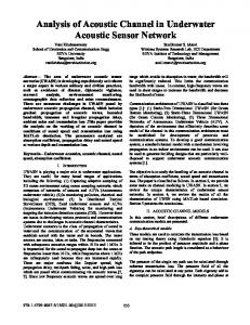
A. Physical Model Description The model consists of a sound source in the aquatic medium. The Helmholtz equation is solved to acquire sound pressure level values utilizing appropriate boundary conditions at the sea surface and bottom as depicted by figure 1 below.

(

)

(1)

Equation (1) represents the acoustic wave equation Where:

The acoustic pressure ( ) can then be replaced by a timeharmonic wave, i.e. , and this is substituted into equation (1) above to get the Helmholtz equation (2) shown below. Fig. 1: Physical sound source/receiver model

( Figure 1 above shows a point sound source representing a typical marine energy device which is submerged some meters deep in the ocean and from the shore. The acoustic media is characterised by factors that are susceptible to varying parameters such as density, sound speed and temperature. The recipient of the noise emitted by the marine energy device could be a hydrophone or some marine animal. In our case, the harbor seal represents the recipient of the sound signals. The aquatic medium is bounded by a free surface (air) and an elastic bottom surface (soil). The model also comprises of a fluid – structure interface between the liquid medium and the elastic solid sea bed. The sound signals radiate cylindrically from the source. The properties of the model are listed in table 1 below.

Equation (2) above which is the wave equation in the frequency domain is used to compute the frequency response of the model using the parametric solver [14]. 1.

Boundary Conditions (BC) Cylindrical wave radiation was applied to the side boundary of the acoustic domain according to equation (3)

Value

( Water Depth [m]

50

Source Depth [m]

7

Receiver Depth [m]

15

Water Density [Kgm-3]

997

Bottom Surface Density [Kgm-3]

1600

Sound Speed in Water [ms-1]

1500

(

) (| |)

(

(| |)

( ))

(

)

)

( )

The surroundings were assumed to be a mere continuation of the domain. An incoming wave with sound pressure amplitude is described by the term on the right hand side of the equation (3) and the direction given by the vector . (| |) is equal to ( ) for the case of the cylindrical wave and is the radius from the source to the boundary. The sound source is described by equation (4) below, which is a power point source. Where is the reference pressure and is the speed.

The values from table 1 below are typical values for sound source/receiver models for an acoustic medium in a real life scenario.


(2)

Where:

Table 1. - Parameters of acoustic medium used in the simulation

Parameter

)

99


( 2.

)

= 2√

source do not receive these sound signals. This is because the signals’ sound pressure levels are below their hearing threshold for these frequency values.

(4)

Length and Time Scale An important property for time-harmonic acoustic analysis is the frequency. Therefore for accurate convergence of the solutions, it is paramount that the wavelength (reciprocal of the frequency) be resolved in the mesh. The rule of thumb therefore is that the maximum mesh element be a fraction of the wavelength. Length scale for the model was thus given as:

( )

⁄

,

therefore,

mesh

26 m 101 m Harbour Seal (Kasak, 1998)

110 100 SPL (dB re 1 µPa )

( )

1m 51 m 201 m

size

⁄

90 80 70 60

Where:

50 0

200

400

600

800

1000

Frequency (Hz)

⁄

Fig. 3. Sound pressure level value from sound source. Model with bottom surface influence

.

The audiogram of the harbour seal is also depicted in Fig. 3 above. It could be deduced that certain frequency components could be heard by harbour seals well beyond the 51 m mark. However certain frequency components cannot be heard by the harbour seal even if they go closer than 51m to the sound source.

4. Results/Discussions SPL values of different frequencies were obtained from several points away from the sound source. The result from the model without the bottom surface influence is shown in Fig. 2 below. It can be deduced that sound pressure level values attenuate faster with distance as frequencies increase. Due to the reverberation and interaction of sound signals from the bottom surface, it is difficult to relate the decrease of SPL with distance as a result of frequency in the model with bottom surface influence (see Fig. 3).

1m 51 m 201 m

Fig. 4.a. through 4.f. below show the models with and without the influence of the bottom surface for 3 different frequency values. The interaction of the sound signals with the bottom surface can be seen clearly from the graphs. This causes reverberation of the sound signals and in turn increases the sound pressure levels. This interaction of sound signals with the surface bottom is also depicted in Fig. 5.a. through 5.c. shown in the Appendix of this paper. The SPL values as a function of distance is shown for both models with and without the surface bottom influence.

26 m 101 m Harbour Seal (Kasak, 1998)

110

SPL (dB re 1 µPa)

100

Sound signals bounce off the bottom surface of the acoustic medium and the extent of the reverberations depends on several factors like the individual frequency component. As shown, the higher the frequency component the higher the scattering effect of sound pressure level values as a result of the surface bottom interface.

90 80 70 60

The bottom surface of this model comprises of a soft bottom bed sandy material which gives some allowance for attenuation of sound signals. In the case of a ‘rock bottom’ surface, the SPL values will be more pronounced.

50 0

200

400

600

800

1000

Frequency (Hz)

It is important to note that marine energy devices could be set as an array of multiple devices. Hence the combined SPLvalues will exceed that of a single device. This results in a larger affecting area radius for marine species.

Fig. 2. Sound pressure level value from sound source. Model without bottom surface influence

The audiogram of the harbour seal is above the SPL values for all frequencies at 51 meters from the source for the model without bottom surface influence (see Fig. 2). Habour seals which are approximately 51 m and beyond the sound https://doi.org/10.24084/repqj12.246

100


Range (m)

Fig. 4.c. 500 Hz Frequency model without bottom surface influence

Depth (m)

SPL (dB)

Fig. 4.d. 500 Hz Frequency model with bottom surface influence

SPL (dB)

Depth (m)

SPL (dB)

Depth (m)

Depth (m)

SPL (dB)

Fig. 4.b. 1000 Hz Frequency model with bottom surface influence

Range (m)

Range (m)

Range (m)

Fig. 4.f. 100 Hz Frequency model with bottom surface influence

Fig. 4.e. 100 Hz Frequency model without bottom surface influence


SPL (dB)

Depth (m)

Depth (m)

SPL (dB)

Range (m)

Range (m)

Fig. 4.a. 1000 Hz Frequency model without bottom surface influence

101


5. Conclusions

Acknowledgement

Sound signals comprising of low frequency components emitted from a marine energy device were simulated. An acoustic medium with the inclusion of a surface bottom interface was modelled for the propagation of these sound signals. The surface bottom interface characterised with reverberation of sound signals was shown to have significant effect on the sound pressure levels measured at certain distances away from the sound source.

The author acknowledges the Irish Research Council (IRC) and the Marine and Environmental Sensing Technology Hub (MESTECH) who co -funded the work.

Appendix

[2]

References .

[1]

SPL of 100 Hz as a fuction of distance

SPL (dB re 1 uPa)

110

[3]

100 90

80

[4]

70 60 50 0

50

100

150

200

250

[5]

Distance 1m from Sound Source (m)

with no suface/bottom effect

[6]

with surface/bottom effect

Fig. 5a – Sound pressure level for both models

[7] [8]

SPL of 500 Hz as a fuction of distance 110 SPL (dB re 1 uPa)

100 90 80

[9]

70 60 50 0

50

100

150

200

250


with no suface/bottom effect

[10]


Fig. 5b – Sound pressure level for both models

[11] [12]

SPL of 1000 Hz as a fuction of distance 110 SPL (dB re 1 uPa)

100 90

80

[13]

70 60 50 0

50

100

150

200

250


[14] with no suface/bottom effect


X. Lurton, An introduction to underwater acoustics: principles and applications: Springer, 2002. C. Erbe, R. McCauley, C. McPherson, and A. Gavrilov, "Underwater noise from offshore oil production vessels," The Journal of the Acoustical Society of America, vol. 133, pp. EL465-EL470, 2013. T. P. Lloyd, V. F. Humphrey, and S. R. Turnock, "Noise modelling of tidal turbine arrays for environmental impact assessment," 2011. S. Patrício, C. Soares, and A. Sarmento, "Underwater noise modelling of wave energy devices," Proc. 8th EWTEC, pp. 1020-1028, 2009. E. de Sousa Costa and E. B. Medeiros, "Mecánica Computacional, Volume XXIX. Number 22. Interdisciplinary Topics in Mathematics (C)," 2010. A. Ivakin, "Modelling of sound scattering by the sea floor," Le Journal de Physique IV, vol. 4, pp. C5-1095-C5-1098, 1994. D. H. Thomson, Marine mammals and noise: Access Online via Elsevier, 1995. M. Cronin, C. Duck, O. Cadhla, R. Nairn, D. Strong, and C. O'keeffe, "An assessment of population size and distribution of harbour seals in the Republic of Ireland during the moult season in August 2003," Journal of Zoology, vol. 273, pp. 131-139, 2007. J. Tougaard, S. Tougaard, R. C. Jensen, T. Jensen, J. Teilmann, D. Adelung, et al., "Harbour seals on Horns Reef before, during and after construction of Horns Rev Offshore Wind Farm," Vattenfall A/S, 2006. S. P. Robinson and P. A. Lepper, "“Scoping study: Review of current knowledge of underwater noise emissions from wave and tidal stream energy devices”," The Crown Estate2013. P. C. Etter, Underwater acoustic modeling and simulation: CRC Press, 2013. R. Soheilifar, A. M. Arasteh, J. Rasekhi, and A. G. Urimi, "A computer simulation of underwater sound propagation based on the method of parabolic equations," in Proceedings of the WSEAS International Conference on Applied Computing Conference, 2008, pp. 91-97. P. Alexander, A. Duncan, and N. Bose, "Modelling sound propagation under ice using the Ocean Acoustics Library's Acoustic Toolbox," in Acoustics 2012 Fremantle: Acoustics, Development and the Environment, 2012, pp. 1-7. C. Multiphysics, "Comsol Multiphysics Modelling Guide 3.2," ed, September 2005, pp. 26 - 35.

Fig. 5c - Sound pressure level for both models


102
