On the Characterization of Time-Scale Underwater Acoustic Signals Using Matching Pursuit Decomposition Nicolas F. Josso∗, Jun Jason Zhang†, Antonia Papandreou-Suppappola†, Cornel Ioana∗, Jerome I. Mars∗ , C´edric Gervaise‡, and Yann St´ephan§ ∗ GIPSA-lab
/DIS, Grenoble Institute of Technology, GIT, Grenoble, France of Electrical, Computer and Energy Engineering, Arizona State University, Tempe, AZ, USA ‡ E3I2, EA3876, ENSIETA, Universit´e Europ´eenne de Bretagne, 29806 Brest Cedex, France § SHOM, Military Center of Oceanography, Brest, France E-mails:
[email protected],
[email protected],
[email protected],
[email protected]
hal-00444328, version 1 - 6 Jan 2010
† School
Abstract— We investigate a characterization of underwater acoustic signals using extracted time-scale features of the propagation channel model for medium-to-high frequency range. The underwater environment over these frequencies causes multipath and Doppler scale changes on the transmitted signal. This is the result of the time-varying nature of the channel and also due to the relative motion between the transmitter-channel-receiver configuration. As a sparse model is essential for processing applications and for practical use in simulations, we employ the matching pursuit decomposition algorithm to estimate the channel time delay and Doppler scale change model attributes for each propagating path. The proposed signal characterization was validated for sparse channel profiles using real-time data from the BASE07 experiment.
I. I NTRODUCTION The characterization of underwater acoustic signals in terms of propagation medium attributes is essential for a large number of applications, including communications, sonar, and marine environment monitoring. The propagating signal is most often subject to undesirable distortion effects due to the time-varying nature of the ocean environment and also due to the relative motion between the transmitter-channelreceiver configuration. For medium-to-high frequency (500 Hz to 20 kHz) range signal propagation, the distortion can be the result of time delays or multipath as well as Doppler scale changes on the transmitted signal. These distortion effects have been represented using a wideband linear time-varying (LTV) channel model formulation [1]–[3]. This is a representation in terms of a continuously-varying, wideband spreading function that is directly related to the physical nature of the distortions intensity and spread in the channel. In order for this representation to be useful in processing and in providing increased performance by model-inherent diversity paths, a discrete multipath-scale system characterization was proposed in [4]–[6]. Such a characterization can decompose a wideband LTV channel output into discrete time shifts and time scale
changes on the input signal, weighted by a smoothed and sampled version of the wideband spreading function. Although this discrete channel model is appropriate to use when estimating underwater wideband channels, it can also be computationally intensive. This computational cost would especially not be warranted when the wideband spreading function characterizing the channel is sparse. In [7], the estimation of the underwater acoustic channel profile was obtained using a matching filtering operation. Since the motion of the transmitter-channel-receiver configuration is not known a priori, the received signal can be correlated with a family of reference signals with different time delays and Doppler scale factors [8]. In [9], shallow water environment profiles were obtained to investigate the wideband Doppler effect. Also, in [10], a channel estimation approach was used based on matching filtering that was combined with a new motion compensation method based on the use of warping filtering techniques and the wideband ambiguity function. In this paper, we consider sparse underwater channel profiles in the medium-to-high frequency range. Due to the sparsity in the actual physical model of the channel, the transmitted signal will only undergo a small number of multipath and Doppler scale changes. Thus, we propose to use the matching pursuit decomposition (MPD) algorithm [11] that can decompose underwater acoustic signals in the time-frequency plane and provide reduced attribute parameters in terms of time shifts and scale changes to represent the wideband channel. The proposed algorithm will make use of a signal dictionary matched to the channel that is derived following our previous work on the wideband ambiguity function [9], [10]. The paper is organized as follows. Section II presents multipath and the Doppler scale effects on underwater acoustic signals. The implementation of the MPD algorithm is described in Section III, and application of the proposed signal characterization to real data from the BASE07 experiments is presented in Section IV.
II. M ULTIPATH AND D OPPLER S CALE C HANGES ON U NDERWATER ACOUSTIC S IGNALS For most underwater acoustic applications, such as communications, sonar and tomography, the propagating signal is considered to have wideband properties. This is due to the fact that the underwater environment causes time delays and Doppler scale changes on the transmitted acoustic signal. In order to describe the motion effect in a multipath underwater scenario, we consider a stationary receiver and a transmitter moving at a constant speed. We assume that the source emits a signal for 𝑇 seconds while moving at a constant speed 𝑣 along the horizontal 𝑥-axis, as illustrated in Fig. 1. Following a transmission, the 𝑥 component of the source position satisfies ) ( ) ( 𝑣𝑇 𝑣𝑇 ≤ 𝑥 ≤ 𝑥0 + , (1) 𝑥0 − 2 2 where 𝑥0 is the horizontal component of the source position at 𝑇 /2 seconds. We assume that the transmit time 𝑡0 and the receipt time 𝑡 are related by 𝑡0 + 𝜏𝑖 (𝑡0 ) = 𝑡,
hal-00444328, version 1 - 6 Jan 2010
𝑇 𝑇 ≤ 𝑡0 ≤ . (3) 2 2 Equation (2) states that a signal transmitted at time 𝑡0 will be received with a propagation time delay 𝜏𝑖 (𝑡0 ) in the 𝑖th path. When the transmitter moves at a constant speed along the 𝑥-axis, the propagation time delay in Equation (2) is given by [9] 𝑧𝑖2 𝑥𝑖 (𝑡0 ) + , (4) 𝜏𝑖 (𝑡0 ) = 𝑐 2 𝑐 𝑥𝑖 (𝑡0 ) −
where 𝑐 is the constant velocity of sound underwater, 𝑥𝑖 (𝑡0 ) = (𝑥0 − 𝑣𝑖 𝑡0 ) is the horizontal component of the virtual source position, 𝑧𝑖 is the depth of the virtual source in the 𝑧-direction, and 𝑣𝑖 is the speed of the virtual source. Note that by virtual source, we refer to an imaginary source from which the signal appears to have directly arrived. We can assume that the propagation time and the projection of the motion vector in Fig. 1 are constant during transmission provided that the propagation distance is negligible when compared to the separation distance between the source and the receiver. Under this assumption, the propagation time delay 𝜏𝑖 (𝑡0 ) does not depend on the transmit time 𝑡0 and can be approximated by 𝜏𝑖 . This is then given by (5)
After some manipulations, it can be shown that [9] 𝑡0 = 𝜂𝑖 (𝑡 − 𝜏𝑖 ) ,
Mobile transmitter and stationary receiver scenario.
This parameter is given by 𝜂𝑖 =
(
(6)
where 𝜂𝑖 is the scale change parameter of the 𝑖th path that is introduced by the wideband Doppler effect of the channel.
1 𝑧𝑖 𝑐 − 2 𝑐 𝑥2 0 1
1 − 𝑣𝑖
(2)
where 𝜏𝑖 (𝑡0 ) is the time of propagation in the 𝑖th path and the range of possible values of 𝑡0 is given by
𝑧2 𝑥0 + 𝑖 . 𝜏𝑖 = 𝑐 2 𝑐 𝑥0
Fig. 1.
).
(7)
In Equation (6), the term 𝜏𝑖 corresponds to the time-delay associated with the 𝑖th path for a fixed source located at 𝑥 = 𝑥0 . As shown in Fig. 1, the motion vector is projected on the 𝑖th path with declination angle 𝜃𝑖 , thus indicating that each path can be characterized by a unique Doppler scale parameter that is related to the speed 𝑣𝑖 . The 𝑖th path is an amplitudeattenuated, time-delayed and Doppler scaled version of the transmitted signal 𝑠(𝑡). Using Equation (6), the signal received from the 𝑖th path can be expressed as ( ) √ (8) 𝑟𝑖 (𝑡) = 𝑎𝑖 𝜂𝑖 𝑠 𝜂𝑖 (𝑡 − 𝜏𝑖 ) , 𝜂𝑖 ∕= 0. The received signal 𝑟(𝑡) is the sum of all the received paths, 𝑟𝑖 (𝑡). Thus, the received signal is given by 𝑟(𝑡) =
𝑁 ∑ 𝑖=1
𝑟𝑖 (𝑡) =
𝑁 ∑
√ 𝑎𝑖 𝜂𝑖 𝑠(𝜂𝑖 (𝑡 − 𝜏𝑖 )),
(9)
𝑖=1
where 𝑁 is the number of propagation paths and 𝜂𝑖 is the Doppler scale parameter of the 𝑖th path. The received signal characterization in (9) states that, for each path 𝑖, 𝑖 = 1, . . . , 𝑁 , there corresponds a time delay 𝜏𝑖 and a Doppler scale change 𝜂𝑖 . In addition, each delay-scale distorted path 𝑖 is attenuated by the factor 𝑎𝑖 . III. U NDERWATER S IGNAL C HARACTERIZATION U SING M ATCHING P URSUIT D ECOMPOSITION A. Matching Pursuit Decomposition Algorithm The matching pursuit decomposition (MPD) algorithm is an iterative processing method that expands a signal into a weighted linear combination of elementary basis functions (or atoms) chosen from a complete dictionary [11]. The resulting expansion of a finite energy signal 𝑥(𝑡) is given by ∑ 𝛼𝑖 𝑔𝑖 (𝑡), (10) 𝑥(𝑡) = 𝑖
where 𝑔𝑖 (𝑡) is the basis function selected from the MPD dictionary 𝒟 at the 𝑖th MPD iteration and 𝛼𝑖 is the corresponding expansion coefficient. In practical applications, the MPD signal expansion is given by 𝑥(𝑡) =
𝑀−1 ∑
𝛼𝑖 𝑔𝑖 (𝑡) + 𝑝𝑀 (𝑡),
(11)
𝑖=0
where 𝑝𝑀 (𝑡) is the residual signal after 𝑀 MPD iterations such that (𝑀−1 ) ∑ ∣𝛼𝑖 ∣2 + ∣∣𝑝𝑀 ∣∣22 , (12) ∣∣𝑥∣∣22 = 𝑖=0
∫
hal-00444328, version 1 - 6 Jan 2010
and ∣∣𝑥∣∣22 = ∣𝑥(𝑡)∣2 𝑑𝑡. The steps of the MPD iterative algorithm are summarized as follows. At the beginning of the iteration, 𝑝0 (𝑡) = 𝑥(𝑡). Then, at the 𝑖th iteration, 𝑖 = 0, 1, ⋅ ⋅ ⋅ , 𝑀 − 1, the projection of the residue 𝑝𝑖 (𝑡) onto every dictionary element 𝑔 (𝑑) (𝑡) ∈ 𝒟 is computed to obtain ∫ +∞ ( )∗ (𝑑) (𝑑) Λ𝑖 = ⟨𝑝𝑖 , 𝑔 ⟩ ≜ 𝑝𝑖 (𝑡) 𝑔 (𝑑) (𝑡) 𝑑𝑡, (13) −∞
where ∗ denotes complex conjugation. The selected dictionary atom 𝑔𝑖 (𝑡) is the one that maximizes the magnitude of the projection (𝑑)
𝑔𝑖 (𝑡) = argmax ∣Λ𝑖 ∣.
(14)
𝑔(𝑑) (𝑡)∈𝒟
The corresponding expansion coefficients is given by ∫ 𝛼𝑖 = ⟨𝑝𝑖 , 𝑔𝑖 ⟩ =
+∞ −∞
𝑝𝑖 (𝑡)𝑔𝑖∗ (𝑡)𝑑𝑡 ,
(15)
and the residues at the 𝑖th and (𝑖 + 1)th iterations are related as 𝑝𝑖+1 (𝑡) = 𝑝𝑖 (𝑡) − 𝛼𝑖 𝑔𝑖 (𝑡).
(16)
In order to best fit the underwater channel model with multipath-scale signal distortions, the atoms in the dictionary are chosen to be time-delayed and Doppler scale changed versions of the transmitted signal 𝑠(𝑡) as in (8). Specifically, the 𝑖th atom in the dictionary will correspond to 𝑔𝑖 (𝑡) =
√ 𝜂𝑖 𝑠(𝜂𝑖 (𝑡 − 𝜏𝑖 )),
𝜂𝑖 ∕= 0.
(17)
Using this dictionary, which matches the time-scale propagation nature of underwater acoustic channels, with the MPD algorithm, we can obtain highly-localized and sparse signal characterizations. The characterizations will correspond to the expansion parameters (𝛼𝑖 , 𝜂𝑖 , 𝜏𝑖 ), 𝑖 = 0, 1, ⋅ ⋅ ⋅ , 𝑀 − 1, obtained after 𝑀 MPD iterations.
B. MPD Implementation for Signal Characterization In order to truly achieve a parsimonious representation with the MPD, especially when the channel itself is sparse, we need to address some issues on the implementation of the MPD algorithm for use in the underwater signal characterization. The first step is to compute the dictionary 𝒟 for the appropriate range of time delays and scale changes. The atom dictionary 𝒟 needs to represent signals computed as in Equation (17), where 𝑠(𝑡) is the transmitted signal. In [4], a complete and discrete time-scale characterization of wideband time-varying systems was presented, from which the expected time delay and scale change parameters, needed here, can be obtained. Another approach is to consider the Doppler tolerance of known signals and then decide on the range of the scale change parameter according to this tolerance. For example, if a linear frequency-modulated (LFM) chirp signal is transmitted, the Doppler tolerance (i.e., half-power contour) is given by [9], [12], [13] 𝑉𝐷 = ±
2610 knots, 𝑇𝑑 𝑊
(18)
where 𝑇𝑑 is the duration and 𝑊 is the bandwidth of the LFM signal. As the scale change parameter is affected by the source velocity, the velocity parameter sampling rate is chosen as 𝛿𝑣 =
1 𝑉𝐷 . 2
(19)
Let us assume that the expected velocities are bounded in 𝑣 ∈ [𝑉min , 𝑉max ] and the expected time-delays are bounded in 𝜏 ∈ [0, 𝑇𝑡 ], where 𝑇𝑡 is the time delay spread of the channel. Then, the atoms in the dictionary 𝒟 are obtained as ( ) 𝑡 − 𝜏𝑛 1 𝑔𝑚,𝑛 (𝑡) = , (20) 1 𝑠 1 − 𝑣𝑐𝑚 (1 − 𝑣𝑐𝑚 ) 2 where 𝑣𝑚 = 𝑉min +
𝑚 , 2 𝑉𝐷
(21)
and 𝜏𝑛 = 𝑛/𝑓𝑠 .
(22)
Here, 𝑓𝑠 is the sampling frequency, and the integers 𝑚 and 𝑛 satisfy 𝑚 ∈ [1, (𝑉max − 𝑉min ) 2 𝑉𝐷 ] ,
(23a)
𝑛 ∈ [1, 𝑓𝑠 𝑇𝑡 ].
(23b)
As the MPD is a recursive algorithm, the residual energy can be used as the algorithm’s stopping criteria. If the signalto-noise ratio (SNR) of the signal is known, then the MPD can stop iterating when the ratio of the signal energy to the residual energy reaches the SNR. Other plausible stopping criteria include the rate of decrease of the residual energy or a fixed number of iterations based on some prior knowledge on the range of values of the channel parameters.
100
0.32 0.34
80 residual energy (%)
time−delay (s)
0.36 0.38 0.4 0.42 0.44
60
40
20
0.46 0.48
0 1
2
3
4
5 6 MPD iteration
0.5 −4
−2
0 speed (ms−1)
2
4
7
8
9
10
6
Fig. 3. Percentage of the residual energy relative to the total energy of the received signal versus the number of MPD iterations.
Fig. 2. Wideband ambiguity function plane of the simulated multipath propagation. The relative speed is 5 m/s and the separation distance between the source and the receiver is 500 m. The cross symbols represent the maxima detected after each MPD iteration.
1
IV. A LGORITHM S IMULATION W ITH D IFFERENT U NDERWATER C HANNEL M ODELS
hal-00444328, version 1 - 6 Jan 2010
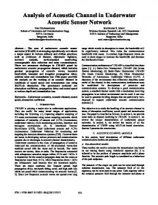
A. Pekeris Waveguide Underwater Channel Model The proposed MPD-based signal characterization was applied to underwater propagation signals that were simulated using the Pekeris waveguide channel model [14]. We developed software that simulate the propagation process based on using ray theory for signals transmitted from a moving source [9]. In order for the simulation to resemble a realistic shallow water scenario, we chose appropriate parameters for the Pekeris waveguide model. Specifically, the water column had a constant sound speed of 1, 500 m/s, 1, 000 kg/m3 density, and 130 m depth. The simulated sea bottom was a flat sandy mud bottom with a sound velocity of 1, 550 m/s and 1, 700 kg/m3 density. The transmitter depth was 24 m, the hydrophone was at 90 m deep, and the range between the transmitter and the receiver was 500 m. The simulated source motion was rectilinear and constant at 5 m/s. The transmitted signal was an LFM with 1,300 Hz central frequency, 2 kHz bandwidth and 4 s duration. The transmitted signal’s bandwidth is very large compared with the signals central frequency. Figure 2 illustrates the results obtained using the MPD algorithm. As we can observe, the wideband ambiguity function of the received signal shows the first seven arrival paths. The multipath profiles obtained using the MPD are illustrated with the wideband ambiguity function as a background in order to show that the expansion parameters (𝜂𝑖 , 𝜏𝑖 ) are coherent and match the local maxima of the wideband ambiguity function. The crosses represent the parameters of the selected MPD atoms after each MPD iteration, from which the expansion coefficients of the decomposition are computed. Specifically, the 𝑖th cross indicates the expansion parameter set (𝜂𝑖 , 𝜏𝑖 ). We observed that the residual energy dropped fast during the first few iterations and then began to decrease slowly, as shown in Fig. 3, which represents the energy of the first ten residues
amplitude
0.8
0.6
0.4
0.2
0 0.32
0.34
0.36
0.38
0.4 0.42 time−delay (s.)
0.44
0.46
0.48
0.5
Fig. 4. Multipath channel profile obtained using three approaches: (a) MPDbased approach (crosses); (b) warping-based lag-Doppler filtering method (solid line); and (c) theoretical approach (circles).
divided by the total energy of the received signal. As expected, the curve of the residual energy follows a logarithmic shape. The MPD-based results are compared to the warping-based lag-filtering (WALF) method in [10] and the comparison is shown in Fig. 4. The multipath profile generated by the MPD algorithm leads to a highly localized, sparse signal characterization (crosses). This sparse profile is comparable to the continuous, motion-compensated channel profile obtained using the WALF method (solid line) and the sparse theoretical channel profile (circles). B. Underwater Acoustic Data from the BASE07 Experiment The BASE07 experiment was jointly conducted by the NATO Undersea Research Center, the Forschungsanstalt der Bundeswehr f¨ur Wasserschall und Geophysik, the Applied Research Laboratory, and the Service Hydrographique et Oc´eanographique de la Marine (SHOM). Two additional days of measurements were also conducted by SHOM to collect data for geoacoustic inversion testing. Results based on the BASE07 experiment can be found at [9], [15]–[17]. The real data we used was collected from a shallow water environment on the Malta Plateau. An LFM signal, whose spectrogram time-frequency representation is illustrated in Fig. 5, was
1
4000
0.8
amplitudes
frequency
3000
2000
0.6
0.4
1000 0.2
0
0.5
1
1.5
2
2.5 time (s)
3
3.5
4
4.5 0
Fig. 5. Spectrogram of the LFM signal (transmitted by a moving source) demonstrating the effects of the mutlipath underwater propagation such as time-delayed echoes.
0.27
0.275
0.28
0.285
0.29 0.295 0.3 delay (sec.)
0.305
0.31
0.315
0.32
Fig. 7. Multipath profile generated by the MPD-based method (crosses) and by the WALF method (solid line).
100
0.25
90 0.26 residual energy (%)
time−delay (s)
hal-00444328, version 1 - 6 Jan 2010
80 0.27 0.28 0.29
60 50 40
0.3
30
0.31 −2
70
−1
0
1
2 speed (m.s−1)
3
4
5
6
Fig. 6. The crosses in the wideband ambiguity function plane represent the time-delay and scale parameters selected after the first 𝑀 = 20 MPD iterations.
transmitted by a source moving rectilinearly at constant speed from 2 to 12 knots and at different depths. The transmitted LFM signal had a 2 kHz bandwidth, 1.3 kHz central frequency, and 4 s duration. Also, the source was moving at a velocity of 2.1 m/s, and the range between the transmitter and the receiver was 1, 300 m. Figure 6 shows the wideband ambiguity function of the received signal, and the crosses correspond to the time-delay and velocity (proportional to scale change) estimates obtained from the first 20 MPD iterations. The multipath profile was obtained from the selected MPD parameters (𝛼𝑖 , 𝜏𝑖 , 𝜂𝑖 ), 𝑖 = 0, 1, . . . , 19. This sparse multipath profile of the channel is represented with crosses in Fig. 7, and each cross corresponds to a multipath-scale path. In the same figure, the solid line represents the multipath profile obtained from the WALF method, and as expected, the two profiles are well-matched. Figure 8 shows that the residual energy decreases logarithmically and approaches the noise level (which was about 20% of the
20
2
4
6
8
10 12 MPD iteration
14
16
18
20
Fig. 8. Percentage of the residual energy relative to the total energy of the received signal versus the number of MPD iterations.
overall signal energy). Although both the MPD-based method and the WALF method result in well-matched signal characterizations, the MPD-based method has some advantages over the other method. One such advantage is that the MPD can accurately recover the original received signal using only a few sets of parameters. Although recovery with the WALF method is still possible, it requires that the paths do not interfere in the wideband ambiguity function plane. For the MPD-based approach, the recovery of the received signal, 𝑟ˆ(𝑡), can be computed using Equation (10) ∑ 𝛼𝑖 𝑔𝑖 (𝑡). (24) 𝑟ˆ(𝑡) = 𝑖
The reconstruction error is then given by ∫ ∣ˆ 𝑟 (𝑡) − 𝑟(𝑡)∣2 𝑑𝑡 ∫ 𝜀= , ∣𝑟(𝑡)∣2
(25)
where 𝑟(𝑡) is the received signal. For the experimental data
ACKNOWLEDGMENT This work was supported by DGA (D´el´egation G´en´erale pour l’Armement) under SHOM research grant N07CR0001 and the Department of Defense MURI Grant No. AFOSR FA9550-05-1-0443.
1
amplitude
0.5
0
R EFERENCES
−0.5
−1 0.5
1
1.5
2
2.5 time (s.)
3
3.5
4
(a) Fig. 9. Time series of the reconstructed signal (solid line) and original received signal (dashed line). 1
amplitude
0.5
0
hal-00444328, version 1 - 6 Jan 2010
−0.5
−1 1.295
1.3
1.305
1.31
1.315 1.32 time (s.)
1.325
1.33
1.335
(a) Fig. 10. Shorter segment, around 1.315 s, of the time series signals in Fig. 9.
example considered here, the reconstruction error after the first 𝑀 = 20 MPD iterations was 𝜀 = 22%; this is close to the ratio of the noise energy over the whole signal energy. The reconstructed signal is illustrated in Fig. 9, with a smaller duration segment plotted in Fig. 10. The time series of the reconstructed signal (solid line) match well (up to the reconstruction error) the time series of the received signal (dashed line).
V. C ONCLUSION We introduced a new approach to characterize a signal propagating over a sparse underwater channel with a stationary receiver and a moving transmitter. The method is based on the use of the matching pursuit decomposition algorithm to extract time-delay and scale change parameters from the received signal, resulting in a highly-localized and sparse signal characterization. This method can be used for active or passive tomography when the source velocity is respectively not wellmonitored or unknown. The new approach was successfully evaluated using simulated data as well as data from the BASE07 experiment.
[1] L. H. Sibul, L. G. Weiss, and T. L. Dixon, ”Characterization of stochastic propagation and scattering via Gabor and wavelet transforms,” Journal of Computational Acoustics, vol. 2, no. 3, pp. 345–369, 1994. [2] R. G. Shenoy and T. W. Park, ”Wide-band ambiguity functions and affine Wigner distributions,” EURASIP Journal on Signal Processing, vol. 41, pp. 339–363, 1995. [3] B. G. Iem, A. Papandreou-Suppappola and G. F. Boudreaux-Bartels, ”Wideband Weyl symbols for dispersive time-varying processing of systems and random signals,” IEEE Transactions on Signal Processing, vol. 50, pp. 1077–1090, May 2002. [4] Y. Jiang and A. Papandreou-Suppappola, “Discrete time-scale characterization of wideband time-varying systems,” IEEE Transactions on Signal Processing, vol. 54, no. 4, pp. 1364–1375, April 2006. [5] S. Rickard, ”Time-frequency and Time-scale Representations of Doubly Spread Channels,” Princeton University, November 2003. [6] A. Papandreou-Suppappola, C. Ioana, and J. J. Zhang, “Time-scale and dispersive processing for time-varying channels,” in Wireless Communications over Rapidly Time-Varying Channels (F. Hlawatsch and G. Matz, eds.). Academic Press, 2009. [7] F.B. Jensen, W.A. Kuperman and H. Schmidt, “Computational Ocean Acoustics,” AIP Press, New York, 1994. [8] J.P. Hermand and W.I. Roderick, “Delay-Doppler resolution performance of large time-bandwidth-product linear FM signals in a multipath ocean environment,” The Journal of the Acoustical Society of America, vol. 84, pp. 1709–1727, 1988. [9] N.F. Josso, C. Ioana, J. I. Mars, C. Gervaise, and Y. Stephan, “On the consideration of motion effects in the computation of impulse response for underwater acoustics inversion,” The Journal of the Acoustical Society of America, accepted for publication, 2009. [10] N.F. Josso, C. Ioana, C. Gervaise, Y. Stephan, and J.I. Mars, “Motion effect modeling in multipath configuration using warping based lagDoppler filtering,” IEEE Trans. Acoust., Speech, Signal Process., pp. 2301–2304, 2009. [11] S. G. Mallat and Z. Zhang, “Matching pursuits with time-frequency dictionaries,” IEEE Transactions on Signal Processing, vol. 41, no. 12, pp. 3397–3415, Dec. 1993. [12] S. Kramer, “Doppler and acceleration tolerances of high-gain, wideband linear FM correlation sonars,” Proceedings of the IEEE, vol. 55, pp. 627– 636, 1967. [13] B. Harris and S. Kramer, “Asymptotic evaluation of the ambiguity functions of high-gain fm matched filter sonar systems,” Proceedings of the IEEE , vol. 56, pp. 2149–2157, 1968. [14] C.L. Pekeris, “Theory of propagation of explosive sound in shallow water,” Propagation of Sound in the Ocean, Memoir 27,” pp. 1-117, Geological Society of America, New York, 1948. [15] G. Theuillon and Y. Stephan, “Geoacoustic characterization of the seafloor from a subbottom profiler applied to the BASE’07 experiment,” The Journal of the Acoustical Society of America, vol. 123, no. 5, pp. 3108–3108, 2008. [16] N. Josso, C. Ioana, C. Gervaise, and J.I. Mars, “On the consideration of motion effects in underwater geoacoustic inversion,” Acoustical Society of America Journal, vol. 123, pp. 3625, 2008. [17] N.F. Josso, C. Ioana, J.I. Mars, C. Gervaise, and Y. Stephan, “Warping based lag-Doppler filtering applied to motion effect compensation in acoustical multipath propagation,” Acoustical Society of America Journal, vol. 125, pp.2541, 2009.