Modelling the Regenerator for Multi-Objective Optimisation of the Air ...

Spreadsheets in Education (eJSiE) Volume 9 | Issue 2

Article 5

5-22-2016

Modelling the Regenerator for Multi-Objective Optimisation of the Air-Bottoming Cycle with Excel Mohamed Musaddag El-Awad Dr Mechanical engineering department, Faculty of Engineerin, University of Khartoum, [email protected]

Follow this and additional works at: http://epublications.bond.edu.au/ejsie

This work is licensed under a Creative Commons Attribution-Noncommercial-No Derivative Works 4.0 License. Recommended Citation El-Awad, Mohamed Musaddag Dr (2016) Modelling the Regenerator for Multi-Objective Optimisation of the Air-Bottoming Cycle with Excel, Spreadsheets in Education (eJSiE): Vol. 9: Iss. 2, Article 5. Available at: http://epublications.bond.edu.au/ejsie/vol9/iss2/5

This Regular Article is brought to you by the Bond Business School at ePublications@bond. It has been accepted for inclusion in Spreadsheets in Education (eJSiE) by an authorized administrator of ePublications@bond. For more information, please contact Bond University's Repository Coordinator.

Modelling the Regenerator for Multi-Objective Optimisation of the AirBottoming Cycle with Excel Abstract

Spreadsheet software can be utilised in energy-related courses to enhance the students’ problem-solving skills and to train them for future research efforts. In this respect, the present paper demonstrates the capabilities of Microsoft Excel for conducting thermodynamics and heat-transfer optimisation analyses of energy systems by considering the air-bottoming power-generation cycle. The paper presents a model that uses the effectivenessNTU method to explicitly take into consideration the design particulars of the regenerator, such as its size and overall heat-transfer coefficient. The study, which uses the exact method of analysis, compares the effectiveness-NTU model with the usual effectiveness (ε) model for multi-objective optimisation of the airbottoming cycle. Keywords

Thermal-fluid systems, optimisation analysis, property add-ins Distribution License

This work is licensed under a Creative Commons Attribution-Noncommercial-No Derivative Works 4.0 License.

This regular article is available in Spreadsheets in Education (eJSiE): http://epublications.bond.edu.au/ejsie/vol9/iss2/5

El-Awad: Multi-Objective Optimisation of the Air-Bottoming Cycle

Modelling the Regenerator for Multi-Variable Optimisation of the Air-Bottoming Cycle with Excel Mohamed M. El-Awad Sohar College of Applied Sciences [email protected]

Abstract Spreadsheet software can be utilised in energy-related courses to enhance the students’ problem-solving skills and to train them for future research efforts. In this respect, the present paper demonstrates the capabilities of Microsoft Excel for conducting thermodynamics and heat-transfer optimisation analyses of energy systems by considering the air-bottoming powergeneration cycle. The paper presents a model that uses the effectiveness-NTU method to explicitly take into consideration the design particulars of the regenerator, such as its size and overall heat-transfer coefficient. The study, which uses the exact method of analysis, compares the effectiveness-NTU model with the usual effectiveness (ε) model for multi-variable optimisation of the air-bottoming cycle. Keywords: Thermal-fluid systems, optimisation analysis, Excel, Solver, property add-ins

1. Introduction With the availability of computers and computer software, the desire to meet industrial needs has made computational tools important elements of modern mechanical engineering curricula. Thus, computer-aided design software has replaced traditional methods in structural design analysis and computational fluid dynamics (CFD) software has become indispensable tools for designing fluid systems. By appealing to students more than traditional “chalk and talk” methods, the use of computers and computer software as teaching tools helps to engage the students more actively in the learning process and motivates them to undertake private studies beyond taught classes [1,2]. In this respect, success stories of integrating software packages, such as Matlab, Mathcad, and HYSYS, in various engineering courses have been reported [3-5]. Using computational tools in undergraduate research projects also encourages the students to exercise critical thinking and to appreciate the importance of life-long learning [6]. While even an iterative solution can be an obstacle for students in a traditional computer-less environment, computer-aided methods allow them to conduct more realistic analyses of energy systems by removing the tedium of manual calculation methods [7]. In this respect, the present paper demonstrates the use of Excel for conducting multi-variable optimisation analyses of the air-bottoming (AB) power systems by using a combined thermodynamics and heat-transfer model. Thermodynamic analyses of the AB cycle usually model the regenerator by using a simple effectiveness (ε) model that does not allow for the design particulars of the heatexchanger to be specified. Using the ε-NTU method to determine the exit temperatures of the hot and cold fluids from the regenerator allows the optimisation process to account for the size and other particulars of the regenerator in an explicit

 2003-2012Spreadsheets in Education, Bond University

Published by ePublications@bond, 2016

1

Spreadsheets in Education (eJSiE), Vol. 9, Iss. 2 [2016], Art. 5

manner. The present Excel-based model, which applies the exact variable specificheat method in its formulation, determines the properties of the working fluid by using the multi-substance Thermax add-in [8].

2. The air-bottoming cycle Figure 1 shows a schematic diagram of a power generation system that works on the air-bottoming cycle. In the AB cycle, the energy of the exhaust gases in the top Brayton cycle is transferred to the compressed air of the bottom cycle. According to Korobitsyn [9], the bottom cycle adds 20–30% to the power output, which boosts the combined-cycle efficiency by up to 45%. Unlike the combined Brayton-Rankine cycle, the AB cycle doesn’t require abundant supply of water or expensive water treatment facilities and can be run unmanned. Figure 2 shows the T-s diagram for the AB cycle in which the two compressors and two turbines are assumed to be adiabatic but not isentropic. Fuel C.C.

3

2 Air 1

C

G

T 5 2b

Regenerator

4 4b

3b

Air 1b

Cb

Tb

G

Figure 1: Schematic diagram of the air-bottoming system

Figure 2: T-s diagram for the air-bottoming cycle

Taking the working fluid as pure air, which is treated as an ideal gas, and given the intake air temperature (T1) and the turbine inlet temperature (T3), the compressor work (wc) and turbine work (wt) of the top cycle per each kg of air are given by:

wc  h1  h2 

http://epublications.bond.edu.au/ejsie/vol9/iss2/5

(1)

2

El-Awad: Multi-Objective Optimisation of the Air-Bottoming Cycle

wt  h3  h4 

(2)

Enthalpy values at states 1 and 3 are determined by the temperatures of inlet-air and the combustion chamber, respectively. Enthalpy values at states 2 and 4 are determined from the respective temperatures T2 and T4. The temperatures T2 and T4 themselves are determined by using the variable specific-heat method. According to this method, the relative pressures Pr2 and Pr4 can be calculated from [10]: Pr 2  Pr1  rp

(3)

Pr 4  Pr 3 / r p

(4)

Where Pr1 and Pr3 are the relative pressures at T1 and T3 and rp is the pressure ratio (P2/P1) in the top cycle. The heat input in the combustion chamber per kg of inlet air (qin) is obtainable from:

q in  h3  h2 

(5)

Similarly, the compressor work (wcb) and turbine work (wtb) per unit mass flow in the bottom cycle can be calculated from:

wcb  h1b  h2b 

(6)

wtb  h3b  h4b 

(7)

The relative pressures Pr2b and Pr4b can be calculated from: Pr 2b  Pr1b  rpb

(8)

Pr 4b  Pr 3b / r pb

(9)

Where Pr1b and Pr3b are the relative pressures at T1b and T3b, respectively, and rpb is the pressure ratio (P2b/P1b) in the boom cycle. Assuming that mb kilograms of air go through the bottom cycle for each kilogram of air in the top cycle, the overall net work (wnet) is given by:

wnet  wt  wc   mb wtb  wcb 

(10)

The overall thermal efficiency of the combined AB cycle (η) is then obtained from:



wnet qin

(11)

3. Modelling the regenerator The regenerator is a key component in the air-bottoming system that strongly affects its performance and economic feasibility. Therefore, appropriate modelling of the regenerator is particularly important in the analyses of the air-bottoming cycle. Thermodynamic analyses usually adopt a simple effectiveness (ε) model for the regenerator, but computer-based methods enable more realistic models that allow multi-variable optimisation of the energy system with respect to its efficiency, cost, size, etc.

Published by ePublications@bond, 2016

3

Spreadsheets in Education (eJSiE), Vol. 9, Iss. 2 [2016], Art. 5

3.1. The effectiveness model Figure 1 shows the regenerator as a counter-flow heat exchanger in which the hot exhaust gas from the top cycle enters at T4 and the cold air from the compressor of the bottom cycle enters at T2b. The effectiveness model determines the exit temperature of the bottom air (T3b) from [10]: T3b  T2b   T4  T2b 

(12)

500

0.5

400

0.4

300

0.3

200

0.2

w_n… η

100

0.1

0

Thermal efficiency

Net specific work (kJ/kg)

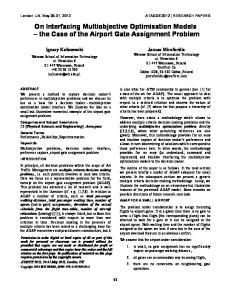
Where ε is the heat-exchanger’s effectiveness, which is below 0.85 for most heat exchangers used in practice [10]. The simple heat-exchanger effectiveness method expressed by Equation (12) is not suitable for modelling the regenerator in the airbottoming cycle which is complicated by the fact that the hot and cold air mass flow rates and their specific heats may differ by large margins. If Equation (12) were used without modification, the variation of the net specific work and thermal efficiency with the mass flow rate in the bottom cycle (mb) will be as shown in Figure 3. The figure indicates that both the thermal efficiency and net work of the bottom cycle continuously decreasing with increasing the ratio of mass flow ratio (mb) and, therefore, the optimum value for mb is zero.

0 0

0.5

1

1.5

2

Ratio of mass flow rates (mb) Figure 3: Variation of the net specific work and thermal efficiency with the ratio of mass flow rates

An improved effectiveness model that takes into consideration the heat capacities in the top and bottom cycles (Ch and Cc, where C=mcp) was used by Czaja et al [11]. According to this model, the temperatures of the two streams leaving the heatexchanger (T3b and T5) are determined from those of the two streams entering the heat-exchanger (T2b and T4) by the following relationships: T3b  T2b   T4  T2b 

If Cc < Ch

(13)

T5  T4   T4  T2b 

If Cc ≥ Ch

(14)

Energy balance over the heat exchanger determines the enthalpy of the exhaust gas in the top cycle as: h5  h4  mb h3b  h2b 

(15)

Assuming a constant specific heat, Equation (15) can be approximated by:

T5  T4  mb T3b  T2b 

(16)

Rearranging:

http://epublications.bond.edu.au/ejsie/vol9/iss2/5

4

El-Awad: Multi-Objective Optimisation of the Air-Bottoming Cycle

T3b  T2b 

1 T4  T5  mb

(17)

Substituting for T5 from Equation (14) into Equation (17), yields:

T3b  T2b 

 mb

T4  T2b 

(18)

Therefore, with this modified ε-model, the temperature T3b is obtained as follows:

T3b  T2b   T4  T2b 

T3b  T2b 

 mb

T4  T2b 

Cc < Ch

(19)

Cc ≥ Ch

(20)

3.2. The effectiveness-NTU model The effectiveness model described in the previous section doesn’t explicitly take into consideration the heat exchanger’s type and size. A more realistic model for the regenerator can be developed by applying the heat-transfer effectiveness-NTU method to determine the exit temperatures from the heat-exchanger [12]. According to this method, the rate of heat-transfer between the two streams (Q) is obtained by the following formula [13]: Q = ε Qmax

(21)

Where, ε is the heat-exchanger effectiveness and Qmax is the maximum possible rate of heat-transfer as given by: Qmax = Cmin (Thi - Tci)

(22)

Where Cmin = MIN(Ch, Cc). Figure 4 shows two arrangements of a single pass, crossflow heat exchanger that can be used as the regenerator of the AB system.

(a)

(b)

Figure 4: Two arrangements of a cross-flow heat exchanger (adopted from [13])

The two arrangements shown in Figure 4 have different formulae for calculating the effectiveness. For example, the effectiveness of the heat exchanger shown in Figure 4.a (both streams unmixed) is determined by [13]:  NTU 0.22

  1  exp 

c

exp cNTU   1 0.78



(23)

Where, NTU stands for the number of transfer units:

Published by ePublications@bond, 2016

5

Spreadsheets in Education (eJSiE), Vol. 9, Iss. 2 [2016], Art. 5

NTU  AU / C min

(24)

c  Cmin / Cmax

(25)

In Equation (24), A is the surface are of the heat exchanger and U is its overall heat transfer coefficient. Since the values of ε for different types of heat exchangers are obtained by using relevant formulae, this model takes into consideration the type of the heat exchanger and the flow patterns of the two fluids [13]. Once Q is determined from Equation (21), the exit temperatures of the two streams can be obtained from: Tco =Tci+ Q /Cc

(26)

Tho =Thi –Q /Ch

(27)

The exit temperatures obtained by the ε-NTU method can now be used in the analytical model of the AB cycle. Accordingly, the temperature T3b in Figure 1 is assigned the value of Tco calculated from Equation (26) and T5 is assigned the value of Tho calculated from Equation (27). 4. The computer model Determination of the pressure ratio (rpb) and mass flow rate (mb) in the bottom cycle that maximise the overall thermal efficiency of the AB cycle requires an optimisation process that suits a computer-based solution method. The computer model developed for the present study uses Excel as a modelling platform. Two Excel sheets were developed for the two alternative models of the regenerator. Fluid properties (h, Pr, cp) at various temperatures are determined by using the Thermax add-in [8]. To illustrate the optimisation process, consider a gas-turbine power plant that operates on a simple Brayton cycle which is to be retrofitted with a bottoming gas turbine. The pressure ratio of the original plant is 10 and the turbine inlet temperature is 1400 K. Intake air to the compressors of both top and bottom cycle is at ambient temperature and pressure of 298.15 K and 103.1 kPa, respectively. The isentropic efficiency for both compressors is 0.85 while that for both turbines is 0.87. Figure 5 shows the sheet developed for the ε-model in which the upper part includes the basic data and calculations for the top cycle while the lower part stores the data of the bottom cycle and its calculations. A value of ε = 0.85 is used. The formula tab in the sheet reveals the formula used to determine the regenerator exit temperature T3b. Figure 5 shows that per 1 kg of air the top cycle requires 891.2479 kJ of heat input (Q_in) to produce 288.1597 kJ of net work (w_nett). Therefore, the thermal efficiency of the top cycle standing alone (η_top) is 0.323322. For the bottom cycle, the sheet shows the calculations for a pressure ratio (P_ratiob) of 5 and mass ratio (mb) of 1. The exhaust gas leaves the top cycle (T_4) at 870.182 K and passes part of its energy to the compressed air of the bottom cycle that enters the heat exchanger (T_2b) at 499.5133 K and leaves (T_3b) at 814.5817 K. The heated air then expands in the bottom cycle turbine to produce a net work (w_netb) of 60.93141 kJ per kg of air flow in the bottom cycle. The overall thermal efficiency (η_ABC) at the specified pressure ratio is 0.391688, which is higher than that of the top cycle alone by about 21%.

http://epublications.bond.edu.au/ejsie/vol9/iss2/5

6

El-Awad: Multi-Objective Optimisation of the Air-Bottoming Cycle

Figure 5: Excel sheet for energy analysis of the AB cycle with the ε-model

Figure 6: Excel sheet for energy analysis of the AB cycle with the ε-NTU model

Figure 6 shows the sheet developed for the ε-NTU model which adds the data and calculations involved in the ε-NTU method as shown on the right side of the sheet. In this model, the area (A) and overall heat-transfer coefficient (U) of the heat exchanger have to be specified. For a gas-to-gas heat exchanger, the range of U is 1040 W/m2.oC [13]. In the present analysis, U is taken as 30 W/m2.oC. The area A is specified such that the exit temperature of the hot-air in the bottom cycle (T3b) is the same as that obtained by the effectiveness model, i.e. 814.58K. The corresponding surface area (obtained by Goal-Seek) is 467.7 m2. Note that the values of the net work and overall thermal efficiency calculated by this model are identical to those obtained by the ε-model. The formula ribbon here reveals how the temperature T3b is assigned the absolute value of Tc,o as calculated by the ε-NTU method: T_3b = T_co+273

(28)

The conversion of T_3b from Celsius to absolute degree is required by the ideal-gas analysis of the AB cycle.

Published by ePublications@bond, 2016

7

Spreadsheets in Education (eJSiE), Vol. 9, Iss. 2 [2016], Art. 5

5. Cycle optimisation analyses The two Excel sheet described in the previous section that apply the two regenerator models will be now be used to determine the optimum pressure ratio and mass flow rate for the bottom cycle by studying the effects of these parameters on the net work from the AB cycle and its thermal efficiency. 5.1. Effect of the pressure ratio

360

0.4

350

0.39

340

0.38

330

0.37

320

w_net

0.36

310

η

0.35

300

Thermal efficiency

Net specific work (kJ/kg)

Keeping the mass flow ratio of air in the bottom cycle (mb) equal to 1, the two sheets were used to determine the variation of the combined net specific work (w_net) and thermal efficiency (η_ABC) with the pressure ratio of the bottom cycle (rpb). Figures 7 and 8 show the results obtained by the two regenerator models. Both figures indicate that the maximum net work and the maximum thermal efficiency occur at the same pressure ratio which is ≈ 4.

0.34 0

2

4 6 Pressure ratio

8

10

360

0.4

350

0.39

340

0.38

330

0.37

320

0.36

w_net η

310

0.35

300

Thrmal efficiency

Net specific work (kJ/kg)

Figure 7: Effect of the bottom-cycle pressure ratio (rp) on the combined net specific work and thermal efficiency with the ε-model

0.34 0

2

4

6

8

10

Pressure ratio in the bottom cycle Figure 8: Effect of the bottom-cycle pressure ratio (rp) on the combined net specific work and thermal efficiency with the ε-NTU model

5.2. Effect of the mass flow-rate With the pressure ratio in the bottom cycle fixed at 4, the two sheets were then used to determine the variation of the combined net specific work (w_net) and thermal efficiency (η_ABC) with the mass flow ratio in the bottom cycle (mb). Figures 9 and 10 show the results obtained at selected values of the air flow ratio in the cycle 0.2 ≤ mb≤1.8. Unlike Figure 3, the two figures indicate that there is an optimum value for mb at which the AB cycle yields its maximum net specific work and thermal efficiency. Both figures indicate that the ratio of air in the bottom cycle per each kg of

http://epublications.bond.edu.au/ejsie/vol9/iss2/5

8

El-Awad: Multi-Objective Optimisation of the Air-Bottoming Cycle

360

0.4

350

0.39

340

0.38

330

0.37

w_net η

320 310

0.36 0.35

300

Thermal efficiency

Net specific work (kJ/kg)

air in the top cycle is about 1.2 kg, but the ε-NTU method shows a smoother variation with mb than the ε-model and yields significantly higher values of w_net and η_ABC at values of mb greater than the optimum value. Estimates of the optimum values of rpb and mb can be improved by repeating the calculations starting with the newly determined value of mb = 1.2.

0.34 0

0.5 1 1.5 Ratio of mass flow rates (mb)

2

360

0.4

350

0.39

340

0.38

330

0.37

320

0.36

w_net η

310

0.35

300

Thermal efficiency

Net specific work (kJ/kg)

Figure 9: Effect of mass flow ratio on the net specific work and thermal efficiency with the ε-model

0.34 0

0.5

1

1.5

2

Mass flow in bottom cycle (mb) Figure 10: Effect of mass flow ratio on the net specific work and thermal efficiency with the ε-NTU model

5.3. Cycle optimisation with Solver The combination of rp and mb that optimises either the overall thermal efficiency or the net specific work of the air-bottoming cycle can be determined easily and accurately by using the Solver add-in. Solver allows Excel to find the maximum or minimum value of the function in a “target cell” by modifying the values stored in the “changing cells”. Figure 11 shows the set-up for Solver for optimising the overall thermal efficiency (η_ABC).

Figure: 11 Solver set-up to maximise the overall efficiency

Published by ePublications@bond, 2016

9

Spreadsheets in Education (eJSiE), Vol. 9, Iss. 2 [2016], Art. 5

As calculated by the sheet using the ε-model, the values determined by Solver for the combination of pressure ratio and mass flow ratio that maximise the overall thermal efficiency, are 2.88 and 1.086, respectively. At these values of rpb and mb, the net specific work and overall thermal efficiency are 353.96 kJ/kg and 0.397, respectively. The corresponding values calculated by the sheet using the ε-NTU model are 3.80 and 1.097, at which the net specific work and overall thermal efficiency are 353.44 kJ/kg and 0.397, respectively. Although the maximum values of w_net and η_ABC obtained by the two models are almost identical, the ε-model obtains these values at a much lower value of the pressure ratio (2.88) compared to the ε-NTU model (3.8).

6. Conclusions With its wide distribution, ease of use, and powerful graphics tools, Excel can be utilised to introduce the basic concepts in introductory energy-related courses. The Thermax property add-in enables the spreadsheet to be used as an open modelling platform for thermal-fluid systems that helps students in advanced energy-related courses to conduct design projects of energy systems. In this respect, the paper presents a case study that demonstrates the advantages of using Excel in the optimisation analysis of the air-bottoming gas-turbine cycle. The example shows that the integration of thermodynamic and heat-transfer methods enables us to develop more useful models of thermal-fluid systems. By using the ε-NTU method to model the generator in the air-bottoming cycle, the computer model allows for different types of heat exchangers. Therefore, the optimisation process can take into consideration the economics as well as the compactness of the system. Such studies help students to practice self-learning and to prepare for future energy-related research activities. The present optimisation analysis of the air-bottoming cycle, which used Thermax to apply the variable specific-heat method, can also be performed by using the IdealGas add-in developed at the University of Alabama [14]. In the lack of such property addins, the analysis can be conducted by using the approximate constant specific-heat method of analysis [10].

References [1]

Danielson, S., Tempe, A.Z, Kirkpatrick, A. Ervin, E. (2011), ASME vision 2030: Helping to inform mechanical engineering education, Frontiers in Education Conference (FIE), 2011

[2]

Denton, D. (1998), Engineering Education for the 21st Century. Journal of Engineering Education, Vol. 87, 1998, No. 1, 19-22

[3]

Santana, T. (2007), Computational Tools for Teaching Graduate Courses in Geotechnical Engineering, International Conference on Engineering Education – ICEE 2007, Coimbra, Portugal, September 3 – 7, 2007. Accessed from www.ineer.org/events/icee2007/papers/388.pdf July 15, 2016

http://epublications.bond.edu.au/ejsie/vol9/iss2/5

10

El-Awad: Multi-Objective Optimisation of the Air-Bottoming Cycle

[4]

Ahmadi-Brooghani, Z. (2006), Using Spreadsheets as a Computational Tool in Teaching Mechanical Engineering, Proceedings of the 10th WSEAS International Conference on computers, Vouliagmeni, Athens, Greece, July 13-15, 2006, 305-310

[5]

Oke, S. A. (2004), Spreadsheet Applications in Engineering Education: A Review, Int. J. Engng Ed. Vol. 20, 2004, No. 6, 893-901

[6]

Jemison, W. D., Hornfeck, W. A., Schaffer, J. P. (2001), The Role of Undergraduate Research in Engineering Education. Proceedings of the 2001 American Society for Engineering Education Annual Conference & Exposition 2001, American Society for Engineering Education, Page 6.1036.1-8

[7]

El-Awad, M.M. (2016), Use of Excel’s ‘Goal Seek’ feature for thermal-fluid calculations, Spreadsheets in Education (eJSiE): Vol. 9: Iss. 1, Article 3, 2016.

[8]

El-Awad, M.M. (2015), A multi-substance add-in for the analyses of thermofluid systems using Microsoft Excel, International Journal of Engineering and Applied Sciences (IJEAS), Vol. 2, Issue-3, March 2015, 63-69.

[9]

Korobitsyn, M.A. (1998), New and advanced energy conversion technologies. Analysis of cogeneration, combined and integrated cycles, 1998.

[10] Cengel, Y.A. and Boles, M.A. (2007), Thermodynamics an Engineering Approach, McGraw-Hill, 7th Edition, 2007 [11] Czaja, D., Chmielniak, T., Lepszy, S. (2013), Selection of Gas Turbine Air Bottoming Cycle for Polish compressor Stations, Journal of Power Technologies, Vol. 93, 2013, No. 2, 67–77 [12] Pierobon, L., and Haglind, F. (2014), Design and optimization of air bottoming cycles for waste heat recovery in offshore platforms. Applied Energy, Vol. 118, 2014, 156–165. [13] Cengel, Y. A., and Ghajar, A. J. (2011), Heat and Mass Transfer: Fundamentals and Applications. McGraw Hill, 2011 [14] University of Alabama, Mechanical Engineering, Excel for Mechanical Engineering project. Accessed from http://www.me.ua.edu/excelinme/ index.htm. February 18, 2016.

Published by ePublications@bond, 2016

11