Mathematical Statistics Stockholm University
Modelling variability in longitudinal data using random change point models Annica Dominicus, Samuli Ripatti, Nancy L. Pedersen and Juni Palmgren
Research Report 2006:1 ISSN 1650-0377
Postal address: Mathematical Statistics Dept. of Mathematics Stockholm University SE-106 91 Stockholm Sweden
Internet: http://www.math.su.se/matstat
Mathematical Statistics Stockholm University Research Report 2006:1, http://www.math.su.se/matstat
Modelling variability in longitudinal data using random change point models Annica Dominicus1,2,3, Samuli Ripatti3, Nancy L. Pedersen3,4 and Juni Palmgren2,3 2006 2006 Abstract Some cognitive functions exhibit multiple phases in old age, which motivates the use of a change point model for the individual trajectory. The change point varies between individuals and is treated as random. Illustrating with an application to cognitive function in a Swedish sample, we contrast the random change point model with models within the family of linear random effects models. The focus is on the ability to capture trait variability. We show that the models make different assumptions about the trait variance over the age distribution, and demonstrate that the random change point model is favourable in this respect. The performance of approximate maximum likelihood estimation based on first-order linearization of the random change point model is evaluated. Through simulations we show that the first-order linearization can produce biased parameter estimates even in an ideal situation with many repeated measurements and a balanced study design. We contrast the results with a Bayesian analysis, based on Markov chain Monte Carlo simulation using Gibbs sampling. KEY WORDS: Change point model; Nonlinear mixed model; First-order linearization; Gibbs sampling; MCMC; Cognitive function.
1
E-mail:
[email protected] Dept. of Mathematics, Stockholm University, Stockholm, Sweden 3 Dept. of Medical Epidemiology and Biostatistics, Karolinska Institutet, Stockholm, Sweden 4 Dept. of Psychology, University of Southern California, Los Angeles, CA, USA 2
1
Introduction
The analysis of repeated measures of cognitive function in old age is nontrivial because the development over time for an individual is often nonlinear. Several studies have shown that some cognitive functions are maintained into old age, and a more marked decline is an indication of impending death (McArdle and Anderson, 1990; Schaie, 1996). This phenomenon is referred to as terminal drop (Berg, 1996), and can potentially be captured by a random change point model incorporating individual-specific change points. In this paper, we investigate the properties of, and estimation procedures for, a random change point model with two phases, both exhibiting a linear trend. Our model allows both the trend and the age at transition from the first to the second phase to be individual-specific. In the statistical analysis we focus on the variance of these random components and model the total variance in cognitive abilities over age. We illustrate the model with an application to cognitive data from the Swedish Adoption/Twin Study of Aging (Pedersen et al., 1992). Random change point models have previously been used in several bioscience applications. These include studies of progression of HIV infection using CD4 T-Cell numbers (Lange et al., 1992; Kiuchi et al., 1995), development of prostate specific antigen (PSA) levels as a marker for prostate cancer (Slate and Turnbull, 2000) and cognitive function in old age (Hall et al., 2003; Jacqmin-Gadda et al., 2005). In the previous studies of cognitive function, the focus has been on the mean trajectory in the pre-dementia phase. For example, Jacqmin-Gadda et al. (2005) assess the overall effect of educational level on the cognitive evolution. In contrast, the focus of this paper is on the ability of the random change point model to explain variability in cognitive function, which has previously not been explored. Although the use of nonlinear mixed models, such as the random change point model, has increased in many applied fields, linear mixed models, or linear random effects models (Laird and Ware, 1982), remain very popular for modelling longitudinal data in behavioral sciences. Linear mixed models allow the assessment of the general trend over time as well as the individual variability. Often the main interest is in the mean parameters and individual-specific random effects serve to absorb variation and to give a clearer picture of the average population effect. The main objective for the Swedish Adoption/Twin Study of Aging (SATSA) is to assess the impact of genetic and environmental influences on the aging process. This is possible through variance decomposition based on structural equation models for twin data (e.g. Dominicus, 2003). Our analyses of data from SATSA thus focus on the estimation of variance parameters. More specifically, we wish to capture trait variability as a function of age. As noted by Verbeke and Molenberghs (2000), linear random effects models imply very specific assumptions about the marginal trait variance. We compare the random change point model with 2
the linear and the quadratic random effects models in their ability to explain trait variability. Due to the nonlinearity of the response function in the random change point model, the likelihood does not have a closed-form expression, which complicates maximum likelihood estimation. Possible solutions to this problem include approximate likelihood methods and sampling-based inference methods. The simplest method for approximate maximum likelihood estimation is the ”first-order algorithm”, described by Beal and Sheiner (1982). The procedure is a natural extension of the linearization algorithm for nonlinear regression. Here, the likelihood is approximated by a first-order Taylor expansion of the response function with respect to the random effects about their expected values. Alternative methods for approximate maximum likelihood include the ”conditional first-order algorithm” proposed by Lindstrom and Bates (1990). In previous applications of random change point models, both the first-order approximation (Cudeck and Klebe, 2002) and the conditional first-order approximation (Slate and Turnbull, 2000) have been used. In a Bayesian perspective, the marginal posterior distribution of model parameters is the target, involving integrations over the joint posterior distribution. In sampling-based Bayesian procedures, numerical integration is avoided by taking repeated samples from the conditional posterior distributions for each parameter (or subset of parameters) in turn. One technique for doing this is to use Markov chain Monte Carlo (MCMC) through Gibbs sampling (Geman and Geman, 1984). It involves the construction of a Markov chain that has the posterior distribution of interest as the stationary distribution. Bayesian approaches have been used in several previous applications of random change point models (Smith, 1975; Carlin et al., 1992; Kiuchi et al., 1995; Slate and Turnbull, 2000). In this paper we compare the performance of the first-order approximation and the Gibbs sampler for estimation of random change point models. The first-order approximation is appealing due to its simplicity. It can easily be used for estimation of extended random change point models, incorporating structured random effects, e.g. for modelling twin data. Although it is known that linearization methods for nonlinear mixed models can yield biased estimates, the severity and the direction of the bias for the random change point model have yet not been assessed. In section 2 the random change point model is described, and different parameterizations are compared. The first-order linearization method for approximate maximum likelihood estimation is described in section 3 and Bayesian analysis based on Gibbs sampling is described in section 4. In section 5 we illustrate features of the random change point model by analysing cognitive data from SATSA based on both first-order approximation and Gibbs sampling. A simulation study comparing the performance of the two procedures is presented in section 6. The findings are summarized and discussed in section 7. 3
2
Random change point model
The random change point model with two phases, both exhibiting a linear trend, can be expressed as b
E(yij ) =
+ b11i tij b02i + b12i tij 01i
if tij ≤ τi , if tij > τi ,
where E(yij ) is the expected value of the response, yij , at the jth measurement for the ith individual at time tij . The random effects b01i and b11i describe the individual-specific intercept and slope for the ith individual in the first phase, before the change point at time τi , and b02i and b12i describe the corresponding parameters in the second phase. For many behavioral traits the transition from the first to the second phase will exhibit no jump. Hence, the trajectory is continuous at τi , which requires that b01i + b11i τi = b02i + b12i τi . One of the parameters is thus redundant and can be solved in terms of the other, e.g. b02i = b01i + b11i τi − b12i τi . The original five-parameter model becomes a four-parameter model b
if tij ≤ τi , 01i + b11i tij E(yij ) = b01i + b11i τi + b12i (tij − τi ) if tij > τi . Bacon and Watts (1971) note that this parametrization is not sensitive for detecting changes in slope and suggest a reparametrization to E(yij ) = b0i + b1i (tij − b3i ) + b2i (tij − b3i )sign(tij − b3i ), where sign(z) = −1 if z < 0, sign(z) = 0 if z = 0, and sign(z) = +1 if z > 0. Under this parametrization, the slope is equal to b1i − b2i before the change point, and equal to b1i + b2i after the change point. For individual i, the change point is denoted b3i , b0i is the expected value of the response at the change point, b1i is the average of the two slopes, and b2i is half the difference of the two slopes. Figure 1 explains the model parameters geometrically. In the analysis of cognitive decline in old age, we want to assess the variability in cognitive function as a function of age. Letting eij denote the residual error, our model is of the form yij = b0i + b1i (ageij − b3i ) + b2i (ageij − b3i )sign(ageij − b3i ) + eij .
(1)
The parameters which describe the individual trajectories are specified as the population mean plus an individual-specific random effect measured as a deviation from the mean, e.g. b0i = β0 +η0i . In vector notation, the population mean parameters are denoted β = (β0 , β1 , β2 , β3 )T . The random effects η i = (η0i , η1i , η2i , η3i )T are assumed to follow a multivariate normal distribution with mean zero and variance-covariance matrix Ψ. In principle Ψ can be unstructured. In our application to cognitive decline (section 5), however, we use a constrained model 4
score
b0 b1
b2 b3
time
Figure 1: Parameters in the change point model for a singel individual. leading to a block-diagonal structure of Ψ. The residual errors in (1) are assumed to be independent of each other and of the random effects, and normally distributed with mean zero and constant variance σe2 . The latter assumption seems plausible in our analysis of cognition in old age, but could be relaxed to allow for heterogeneity in residual errors (e.g. Davidian and Giltinan, 1995).
3
First-order linearization for approximate maximum likelihood inference
We express all repeated measurements for the ith individual from ni time points as the vector yi = (yi1 , yi2 , ..., yini )T , and write the random change point model (1) as yi = f i (agei , η i , β) + ei , (2) where ei = (ei1 , ei2 , ..., eini )T . The function f i is nonlinear in both the fixed effects β and the individual-specific random effects η i . The likelihood expression for a sample of m individuals is m Z Y
p(yi |agei , η i ; β, Ψ, σe2 )p(η i |Ψ)dη i .
(3)
i=1
Since the outcome yi is a nonlinear function of η i there is no analytic expression for the marginal distribution of yi in (3). In the first-order linearization, Beal and Sheiner (1982) approximate (2) with the first terms in a Taylor expansion about the expected value of the random effects, i.e. about η i = 0. Retaining the first two terms in the expression gives yi ≈ f i (agei , 0, β) + Fi (agei , 0, β, )η i + ei , 5
(4)
where Fi (agei , 0, β) is the matrix of the first partial derivatives of f i (agei , η i , β) with respect to η i , evaluated at η i = 0. Expression (4) is linear in the random effects η i , and a nonlinear function of the fixed effects β. The important consequence of (4) is that the marginal mean and covariance of yi may be specified readily as: E(yi ) ≈ f i (agei , 0, β), Cov(yi ) ≈ Fi (agei , 0, β)ΨFi T (agei , 0, β) + σe2 Ii ,
(5) (6)
where Ii is the ni × ni identity matrix. If η i and ei are normally distributed, it follows from (4) that the marginal distribution is approximately normal with moments given by (5) and (6). Numerical techniques such as the Newton-Raphson algorithm and its variants can be used for maximum likelihood estimation of the approximate model (4). Under approximation (4) and the assumption that the random effects and the residual errors are normally distributed, inference may be based on standard asymptotic theory for maximum likelihood. For example, the asymptotic variance-covariance matrix for model parameters may be estimated by the inverse of the information matrix evaluated at the estimates. Numerical estimation is facilitated when the mean function is differentiable, so the transition from the first to the second phase is usually smoothed (Seber and Wild, 1989). Bacon and Watts (1971) suggest replacing sign(·) by a smooth function and they describe certain conditions that such a function should obey. We ³ ´ 3j smooth the change point model by replacing sign(tij −b3j ) by tanh tij −b , where γ γ is a small positive smoothing parameter. The values of γ that we consider, all less than one, give similar results, and we use γ = 0.1 in the analyses of empirical and simulated data. In the random change point model for cognitive decline, the smooth transition from the first to the second phase agrees with the clinical belief of a progressive decline.
4
Gibbs sampling for Bayesian inference
An alternative to the likelihood approach is to take a Bayesian perspective and perform Markov chain Monte Carlo (MCMC) simulations to approximate the posterior distribution of the parameters. This involves constructing a Markov chain with the required posterior distribution as its stationary distribution. We use a Gibbs sampler (Geman and Geman, 1984; Gelfand and Smith, 1990) to construct Markov chains. The Markov chains are run for a long time, after which samples from the required distribution can be assembled. We use a Metropoliswithin-Gibbs algorithm for which the full conditional distributions only need to be known up to a normalizing constant. Full Bayesian analysis is conceptually straightforward, albeit computationally demanding.
6
In the three-stage hierachical change point model, the first and second stage models defined in section 2 take the form yi |agei , bi , ωe ∼ MVN(f i (agei , bi ), ωe Ii ) bi |β, Ω ∼ MVN(β, Ω), where ωe (σe−2 ) is the residual precision parameter and Ω (Ψ−1 ) is the (4 × 4) precision matrix for the random effects. In the third stage, we use the following prior distributions: β ∼ MVN(β ∗ , H) Ω ∼ Wishart((ρΩ∗ )−1 , ρ) ωe ∼ Gamma(λ1 , λ2 ).
(7)
The hyperparameters β ∗ , H, ρ, Ω∗ , λ1 and λ2 are assumed to be known. Here, λ1 and λ2 are the shape and rate parameters of the Gamma distribution. This choice of priors correspond to proper conjugate distributions, which have the desired property of leading to posterior distributions of known form (e.g. Gelman et al., 2004). In the model given by (1), the random effects are bi = (b0i , b1i , b2i , b3i )T . This parametrization aims at minimizing the correlation between model parameters when drawing from the conditional posterior distributions. In our applications, we also consider restrictions on the covariance structure for the random effects bi . For effects that are assumed to be independent of other effects, we use a normal distribution for the mean parameter, and a Gamma distribution for the precision parameter, as priors. The specific values used for the hyperparameters are given in section 5 and 6.
5 5.1
Application to longitudinal data on cognitive decline Description of the data
We analyze data on cognitive function, measured by the Symbol Digit test, which taps the ability to quickly and accurately compare numbers and symbols (Pedersen et al., 1992). The assessment of cognitive function is part of the Swedish Adoption/Twin Study of Aging (SATSA), a longitudinal twin study of aging that includes both questionnaire assessments and in-person testings of cognitive and functional capabilities, personality and health. The base population of SATSA comprise all twin pairs in the Swedish Twin Registry (Lichtenstein et al., 2002) who indicated that they had been reared apart, and a control sample of twins 7
20 30 40 50 60
Test score
reared together, matched to those reared apart on gender, age and county of birth (3838 individuals). The first in-person testing took place in 1986-1988 and followup data were obtained after three, six, thirteen, and sixteen years. SATSA has been described in detail by Finkel and Pedersen (2004). To avoid the issue of clustered sampling in this illustration, we choose one twin at random from each twin pair. In this sample of 438 individuals, 60% are women and 40% are men. The data are highly unbalanced in that individuals are measured at very different ages. The mean age at the first test occasion (in 1986-1988) for this sample is 62 years, all individuals being in the range of 37–88 years. Because some participants are lost to follow up, or have a late entry into the study, only 98 of the 438 individuals have test scores from all five test occasions. Further, 58 have data from four test occasions, 106 from three test occasions, 102 from two test occasions, while 74 only from one single test occasion. Individuals with few measures contribute with little information in the estimation of parameters in a random effects model. Predictions of individual-specific random effects for these individuals will be close to the population mean estimates. In the analyses, we assume that the missing data mechanism is ”ignorable”, in the sense of Little and Rubin (2002). Although this is a questionable assumption (Pedersen et al., 2003), expanding on this issue is beyond the scope of this paper.
45
55
65
75
Age (in years)
Figure 2: Symbol Digit test scores for 10 participants in SATSA, randomly selected among participants with five repeated scores.
8
Figure 2 shows test score trajectories for 10 individuals randomly selected from those having five repeated scores from the Symbol Digit test. The figure indicates a high within- and between-individual variability, but lacks a clear indication of a particular functional form for a population curve besides an overall decrease in test scores with age.
5.2
Random change point model for cognitive decline
The random change point model (1) is applied to cognitive data from SATSA and estimated using both the first-order approximation and the Bayesian approach. Initial analyses suggest that the change point model with a full covariance structure between all random effects is overparameterized, but indicates a strong correlation between the difference between the two slopes, b2i , and the level at the change point, b0i . We adapt a random change point model including this correlation, and assume independence for all other random effects, leading to a block diagonal structure for Ψ. Age was centered at 65 years. In the Bayesian approach, we use prior distributions for the mean and precision parameters, as follows: Ã
β ∗02
Ã
∼ MVN (40, 0),
0.01 0 0 0.01
β1 ∼ N(0, 0.01) β3 ∼ N(5, 0.1) Ω∗02
∼
à 100 Wishart 2
0
0 0.5
!−1
!!
, 2
ω1 ∼ Gamma(0.1, 0.1) ω3 ∼ Gamma(0.1, 0.1) ωe ∼ Gamma(0.1, 0.1).
This choice of priors is fairly noninformative for both mean and variance-covariance parameters. We find that the choice of hyperparameters in the prior distributions for β and Ω have little influence on the marginal posterior distributions. We run two independent parallel chains of the Gibbs sampler, with different starting values. After a burn-in of 100000 iterations, each sequence was taken to 500000 iterations. The posterior distributions for the mean parameter in β and the variance-covariance parameters in Ψ were obtained by mixing the two sequences. The convergence of the Markov chains was assessed visually and based on Geweke’s convergence diagnostic criterion (Geweke, 1992). The parameter estimates from first-order approximation and MCMC are given in Table 1. The estimates from the two procedures are rather similar, with some important exceptions. The estimates of mean and variability in the difference in 9
slope before and after the change point, β2 and ψ2 , are both estimated to be lower based on the first-order approximation compared to MCMC. Estimates of the variability in level at the change point, ψ0 , and the variability in change points, ψ3 , are also different for the two methods. None of the discrepancies are very large in relation to the uncertainty in parameter estimates, though. The following discussion of parameter estimates will be based on the MCMC results. Kernel density plots of the marginal posterior distributions are displayed in Figure 3. Table 1: Random change point model for cognitive function in SATSA. First-order approx. MCMC Parameter Estimate SE Median Mean SE β0 34.6 0.6 35.2 35.3 1.5 β1 -0.81 0.03 -0.81 -0.81 0.04 β2 -0.14 0.04 -0.16 -0.16 0.05 β3 6.84 0.21 6.39 6.22 1.65 ψ0 88.3 15.8 106 106 13 ψ1 0.038 0.035 0.036 0.038 0.014 ψ2 0.083 0.051 0.15 0.15 0.04 ψ3 35.7 21.5 7.57 11.8 12.5 ψ02 -2.30 0.56 -2.66 -2.68 0.69 σe2 23.2 1.3 22.8 22.8 1.3 The estimates of the population mean parameters, β0 , β1 , β2 and β3 , reflect a general decline in cognitive function measured by the Symbol Digit test. The mean age for the change point is 71 years, the mean slope is -0.65 scores/year before the change point and -0.97 scores/year after the change point. The correlation between an individuals level at change point and difference in slope before and after the change point is equal to -0.67. The negative correlation suggests that individuals having a high level at the change point have a larger (negative) difference in slope for the two phases. The goodness-of-fit of the random change point model is illustrated by the observed versus predicted score ratio in Figure 4. The prediction of scores is fairly good, except for very small values, suggesting that low test scores are more difficult to predict. Figure 2 suggests that there is indeed a fairly large variability in individual trajectories making accurate predictions difficult. To contrast the results from the random change point model, we refit the linear and the quadratic random effect models, which have previously been used to analyze cognitive data from SATSA. Model estimation was based on ML. The left plot in Figure 5 displays the observed mean test score for the SATSA sample as a function of age together with the results from the linear and the quadratic random effects models, and the first-order linearization of the random change point model. The observed mean trajectory is obtained as a moving average. 10
β1
β2
35
40
0
0
0.00 30
−1.0
−0.9
−0.8
−0.7
−0.4
0 10
25
0.025 5
10
0.0 0.1
ψ1
0.000
0.20 0.00
0
−0.2
ψ0
β3
40
80
160
0.00
0.05
ψ3
0.10
0.15
ψ02 0.3
8
0.08
0.6
ψ2
120
0.1
0.2
0.3
0.4
0.0
0
0.00
4
Marginal posterior density
4
4
8
0.20
β0
0
20
40
60
80
−7
−5
−3
−1 0
Parameter value
2.0 1.0 0.0
Observed/Predicted
Figure 3: Marginal posterior distributions for parameters in the random change point model.
0
20
40
60
80
Predicted
Figure 4: Observed/Predicted versus predicted scores based on one draw from the posterior distribution of the individual-specific random effects in the change point model for Symbol Digit scores.
11
40 35
40 35 55
65
75
30
Observed 1st draw 2nd draw 3rd draw 4th draw
25
30
Observed Linear model Quadratic model 1st order approx.
25
Mean score
45
Random change point model
45
Linear random effects models
85
55
65
75
85
Age Figure 5: Observed and predicted mean score trajectories for cognitive function. The predicted mean trajectories for the linear and the quadratic random effects models were calculated based on the ML estimates of the fixed effects in these models. The predicted mean trajectory based on the first-order approximation of the random change point model was derived from (5) using the estimates in Table 1. The right plot in Figure 5 displays the observed mean score trajectory together with four different predicted mean score trajectories obtained from four draws from the posterior distribution of the individual-specific random effects in the random change point model. From Figure 5 it is clear that the observed overall trend is close to linear, and the predicted mean trajectories are all close to the observed mean trajectory. With the original motivation of studying twins to decompose trait variability into variability induced by genetic and environmental factors, the primary goal of this study is to assess the variability in traits. Especially, we are interested in the variability as a function of age. Figure 6 displays the observed variance trajectories together with model induced variance trajectories. The trajectories for the linear and the quadratic random effects models (left plot in Figure 6) were derived analytically. Also the trajectory for the first-order approximation of the random change point model was derived analytically based on the approximate expression (6) using the mean and variance-covariance parameter estimates in Table 1. Without linearizing the model, however, the variance cannot be obtained analytically. Therefore, we use the four draws from the posterior distribution of the random effects to obtain predicted outcomes for the random change point model. Variance trajectories (one for each posterior draw) could then be obtained by calculating the variance of the predictions and add the residual variance in 12
moving age windows (right plot in Figure 6). Figure 6 indicates that the variability in observed test scores increases in the range 60–70 years. Apparently, all the models considered imply very different assumptions about the trait variability, although the mean trajectories in Figure 5 are similar. The variance trajectory predicted from the random change point model approximately follows the observed variance curve. The only discrepancies are in the beginning and in the end of the observed age range, where the available data is limited. In contrast, both the linear and the quadratic variance trajectories are far from the trajectory based on empirical data. The variance trajectory based on the first-order linearization of the random change point model, mimics the observed variability fairly well, except for a peak at the estimated mean age at change point.
140 120 100
100
120
140
Random change point model
55
65
75
Observed 1st draw 2nd draw 3rd draw 4th draw
80
Observed Linear model Quadratic model 1st order approx.
80
Variance of scores
Linear random effects models
85
55
65
75
85
Age Figure 6: Observed and predicted variance trajectories for cognitive function.
6
Simulation study
We investigate the performance of the first-order approximation, implemented in SAS PROC NLMIXED (Wolfinger, 1999), and Gibbs sampling, implemented in WinBUGS 1.4 (Spiegelhalter et al., 2003), by means of Monte Carlo simulation. Parameters used for data generation were chosen to approximately mimic the cognitive decline observed in SATSA. For simplicity, we use a balanced data design and assume the random effects to be independent. Four settings are considered, differing only in the number of repeated measurements and the variance of individual-specific change points, ψ3 :
13
Setting Time points ψ3 1 −6, −5, ..., 6 4 2 −6, −3, 0, 3, 6 4 3 −6, −5, ..., 6 25 4 −6, −3, 0, 3, 6 25 Setting 1 is an ideal situation with all individual-specific change points being within the observed time range, and the thirteen repeated measures being centered around the mean change point. Setting 2 is similar to the first, except the data is reduced to five repeated measurements. In setting 3 the variance of the individualspecific change points is increased to 25 years. With time points centered around zero, and individuals being observed once a year between -6 and 6, a standard error of 5 means that on average only 31% of the individuals have their change point inside the observed time range (individual-specific change points are assumed to be normally distributed). Setting 4 is the worst case with both a large variability in change points and only five repeated measures for each individual. The simulations of the first-order approximation were based on 200 samples, each including 500 individuals. The maximum number of iterations for estimation of each sample was set to 200. The starting values were chosen to lie close to the true values to improve convergence. Due to the computational burden of estimation through MCMC simulation, the number of samples was reduced to 20 (each including 500 individuals) in the evaluation of the performance of the Gibbs sampler. The prior distributions for the model parameters were chosen to be vague: β0 β1 β2 β3 ω1 ω2 ω3 ω4 ωe
∼ ∼ ∼ ∼ ∼ ∼ ∼ ∼ ∼
N(40, 0.01) N(0, 0.01) N(0, 0.01) N(0, 0.01) Gamma(0.001, 0.001) Gamma(0.001, 0.001) Gamma(0.001, 0.001) Gamma(0.001, 0.001) Gamma(0.001, 0.001).
The results from simulations based on the first-order approximation (Table 2) reveal that both the mean and the variance of the difference in the two slopes, β2 and ψ2 , are underestimated with up to 53% and 63%, respectively. The bias is present even in the best situation, with thirteen yearly measurements for all individuals, and all individual change points being in the observed time range. When 14
decreasing the number of repeated measurements, and increasing the variability in change points, the bias increases. With large variability in individual change points, the variability in average slope, and level at the change point, are overestimated. With only five repeated measurements, the variability in individual change points is also overestimated. The mean of estimated standard errors and the empirical standard errors are similar for most parameters, except for the mean change point, β3 , where the estimated standard error is substantially smaller than the empirical standard error. The simulation results based on the MCMC method, also given in Table 2, suggest that the Gibbs sampler performs well in all four settings considered. The means of the medians of posterior parameter distributions are all close to the true parameter values even in the worst setting. As expected, the variability in posterior medians for β3 and ψ3 increases as the variability in change points increases.
7
Discussion
We have demonstrated the use of random change point models for modelling variability in longitudinal data. Although neglected in many applications of linear random effects models, it is well known that the form of the random effects model has implications for the variance structure (e.g. Verbeke and Molenberghs, 2000). This is especially problematic in applications where the primary interest is in the trait variance, which is typically the case in family studies. Based on an empirical study of cognitive function in old age, we showed that the random change point model is very flexible in capturing the trait variability as a function of age. This is in contrast to the linear and the quadratic models, which are often used in analyses of longitudinal family data. We evaluated two procedures for estimation of the random change point model, the first-order linearization for approximate maximum likelihood estimation and a Bayesian approach based on Gibbs sampling. Both procedures have previously been used in applications of random change point models, and are easy to implement. Through simulations we showed that individual-specific trajectories are biased towards a linear curve when estimation is based on the first-order approximation. As anticipated, the bias increased when the variability in the individual-specific change points increased. Refinements of the first-order approximation for approximate ML estimation of nonlinear mixed models, such as the conditional first-order algorithm proposed by Lindstrom and Bates (1990), are expected to reduce bias in parameter estimates. The difference in results between the first-order and the conditional first-order analyses will decrease as the number of observations per individual decreases, however. The reason is that the empirical Bayes estimates of the random effects
15
are ’shrunk’ towards the mean value of zero, and this shrinkage is greater the smaller the amount of data is available for each individual. A Bayesian analysis based on Gibbs sampling seems to be a useful alternative for making inference about the random change point model. In our simulations, the medians of the marginal posterior distributions of model parameters were all close to the correct values, even with a moderate amount of data (500 individuals observed at five occasions). However, it is yet not clear how noninformative prior distributions for the variance-covariance parameters should be chosen. Gelman (2005) argues that the inverse-gamma distribution typically used for being noninformative for a variance parameter, may have problems. Instead, a uniform prior on the hierarchical standard deviation is recommended. The generalization to priors for a multivariate nonlinear hierarchical model, such as the random change point model, merits further investigation. In spite of the fairly complex structure of the random change point model, it may still not capture all features of cognitive evolution. For example, censored change points are not explicitly modelled. In studies of cognition in old age, loss to follow-up is also a reality. If the dropout is ”non-ignorable” it has to be accounted for explicitly to avoid selection bias. Jacqmin-Gadda et al. (2005) adapted a random change point model for cognitive decline tied to a survival model for dementia to address this issue. The motivation for this work was a longitudinal twin study of cognition with the ultimate goal of decomposing the variability in individual trajectories into variability due to genetic and environmental factors. Neale and McArdle (2000) describe a method for variance decomposition for nonlinear random effects models for longitudinal twin data based on a first-order approximation of the response model. This procedure is appealing since the approximate model is a structural equation model, and standard procedures for ML estimation can be used. However, our results indicate that the first-order approximation of the random change point model may yield biased estimates of both mean and variance-covariance parameters. A random change point model for twin data should therefore be based on another approach, e.g. the Bayesian approach discussed in this paper. Open questions for this extended model include the choice of priors, especially for the covariance matrix. The implications of the distortion of the orthogonality of the mean and covariance structure for the individual-specific random effects, due to the nonlinearity of the regression model, will also have to be carefully assessed.
16
17
(−6, −5, ..., 6) MCMC Est. Mean SE 45.01 0.40 -0.51 0.03 -0.29 0.03 -0.06 0.16 75.56 4.94 0.30 0.02 0.30 0.02 3.89 0.61 1.00 0.02 (−6, −5, ..., 6) MCMC Est. Mean SE 44.82 0.47 -0.50 0.03 -0.29 0.03 -0.03 0.45 77.25 5.70 0.32 0.03 0.30 0.03 22.90 3.36 1.00 0.02
Time points = First-order approx. Est. Emp. Mean SE SE 43.97 0.44 0.48 -0.50 0.03 0.03 -0.14 0.02 0.02 0.02 0.06 0.37 95.65 6.17 6.85 0.48 0.03 0.03 0.12 0.01 0.01 8.45 2.43 2.77 1.08 0.02 0.02
True value 45 -0.5 -0.3 0 75 0.3 0.3 4 1
True value 45 -0.5 -0.3 0 75 0.3 0.3 25 1
β0 β1 β2 β3 ψ0 ψ1 ψ2 ψ3 σe2
β0 β1 β2 β3 ψ0 ψ1 ψ2 ψ3 σe2
Emp. SE 0.40 0.04 0.03 0.45 4.65 0.03 0.03 3.39 0.02
Emp. SE 0.56 0.02 0.03 0.15 4.21 0.02 0.02 0.68 0.02 Time points = First-order approx. Est. Emp. Mean SE SE 44.05 0.45 0.49 -0.49 0.03 0.03 -0.15 0.02 0.02 -0.19 0.05 0.53 92.68 6.31 7.12 0.46 0.03 0.04 0.11 0.01 0.02 21.27 7.61 10.89 1.20 0.06 0.06
Time points = First-order approx. Est. Emp. Mean SE SE 44.66 0.40 0.40 -0.50 0.03 0.03 -0.24 0.02 0.02 -0.01 0.01 0.08 76.46 5.05 5.09 0.32 0.02 0.02 0.18 0.02 0.02 11.79 3.76 3.40 1.22 0.06 0.07
Table 2: Simulations on random change point model.
Time points = First-order approx. Est. Emp. Mean SE SE 44.72 0.40 0.40 -0.50 0.03 0.03 -0.25 0.02 0.02 0.01 0.01 0.08 77.67 4.99 5.00 0.34 0.02 0.02 0.21 0.02 0.02 6.12 1.32 1.19 1.07 0.02 0.02 (−6, −3, 0, 3, 6) MCMC Est. Emp. Mean SE SE 45.12 0.46 0.34 -0.49 0.03 0.03 -0.30 0.04 0.05 -0.10 0.48 0.47 75.17 5.68 6.50 0.29 0.03 0.04 0.30 0.03 0.03 26.49 4.67 5.71 1.01 0.05 0.04
(−6, −3, 0, 3, 6) MCMC Est. Emp. Mean SE SE 44.99 0.40 0.42 -0.51 0.03 0.03 -0.30 0.03 0.04 0.04 0.20 0.18 75.31 4.99 4.99 0.29 0.02 0.03 0.30 0.03 0.02 4.21 0.88 0.82 1.00 0.05 0.05
8
Acknowledgements
This work was supported by grants from the Swedish Foundation of Strategic Research (A3 02:129), the Wallenberg Consortium North (WCN2004 Bioinformatic platform KAW2004.0083) and the National Institutes of Health (AG 04563, AG 10175).
References Bacon, D. W. and Watts, D. G. (1971), “Estimating the transition between two intersecting straight lines,” Biometrika, 58, 525–534. Beal, S. L. and Sheiner, L. B. (1982), “Estimating population kinetics,” CRC Critical Reviews in Biomedical Engineering, 8, 195–222. Berg, S. (1996), Aging, behavior, and terminal decline, San Diego: Academic Press, Handbook of the Psychology of Aging, 4th ed., pp. 323–337. Carlin, B. P., Gelfand, A. E., and Smith, A. F. M. (1992), “Hierarchical Bayesian analysis of changepoint problems,” Applied Statistics, 41, 389–405. Cudeck, R. and Klebe, K. J. (2002), “Multiphase mixed-effects models for repeated measures data,” Psychological Methods, 7, 41–63. Davidian, M. and Giltinan, D. M. (1995), Nonlinear Models for Repeated Measurement Data, Boca Raton: Chapman & Hall/CRC. Dominicus, A. (2003), “Latent variable models for longitudinal twin data with dropout and death,” Research report 2003:17, Mathematical Statistics, Stockholm University, Sweden. Finkel, D. and Pedersen, N. L. (2004), “Processing speed and longitudinal trajectories of change for cognitive abilities: The Swedish Adoption/Twin Study of Aging,” Aging, Neuropsychology, and Cognition, 11, 325–345. Gelfand, A. E. and Smith, A. F. M. (1990), “Sampling-based approaches to calculating marginal densities,” Journal of the American Statistical Association, 85, 398–409. Gelman, A. (2005), “Prior distributions for variance parameters in hierarchical models,” Bayesian Analysis, 1, 1–19. Gelman, A., Carlin, J. B., Stern, H. S., and Rubin, D. B. (2004), Bayesian Data Analysis, Boca Raton: Chapman & Hall/CRC, 2nd ed.
18
Geman, S. and Geman, D. (1984), “Stochastic relaxation, Gibbs distributions, and the Bayesian restoration of images,” IEEE Transactions on Pattern Analysis and Machine Intelligence, 6, 721–741. Geweke, J. (1992), Evaluating the accuracy of sampling-based approaches to the calculation of posterior moments, Oxford: Oxford University Press, Bayesian Statistics 4. Hall, C. B., Ying, J., Kuo, L., and Lipton, R. B. (2003), “Bayesian and profile likelihood change point methods for modeling cognitive function over time,” Computational Statistics & Data Analysis, 42, 91–109. Jacqmin-Gadda, H., Commenges, D., and Dartigues, J.-F. (2005), “Random changepoint model for joint modeling of cognitive decline and dementia,” Biometrics, doi:10.1111/j.1541-0420.2005.00443.x. Kiuchi, A. S., Hartigan, J. A., Holford, T. R., Rubinstein, P., and Stevens, C. E. (1995), “Change points in the series of T4 counts proir to AIDS,” Biometrics, 51, 236–248. Laird, N. M. and Ware, J. H. (1982), “Random-effects models for longitudinal data,” Biometrics, 38, 963–974. Lange, N., Carlin, B. P., and Gelfand, A. E. (1992), “Hierarchical Bayes models for the progression of HIV infection using longitudinal CD4 T-cell numbers,” Journal of the American Statistical Association, 87, 615–626. Lichtenstein, P., deFaire, U., Floderus, B., Svartengren, M., Svedberg, P., and Pedersen, N. L. (2002), “The Swedish Twin Registry: a unique resource for clinical, epidemiological and genetic studies,” Journal of Internal Medicine, 252, 184–205. Lindstrom, M. J. and Bates, D. M. (1990), “Nonlinear mixed effects models for repeated measures data,” Biometrics, 46, 673–687. Little, R. J. A. and Rubin, D. B. (2002), Statistical Analysis with Missing Data, Hoboken: Wiley, 2nd ed. McArdle, J. J. and Anderson, E. (1990), Latent variable growth models for research on aging, New York: Academic Press, Handbook of the Psychology of Aging, 3rd ed., pp. 21–44. Neale, M. C. and McArdle, J. J. (2000), “Structured latent growth curves for twin data,” Twin Research, 3, 165–177.
19
Pedersen, N. L., Plomin, R., Nessleroade, J. R., and McClearn, G. E. (1992), “Quantitative genetic analysis of cognitive abilities during the second half of the lifespan,” Psychological Science, 3, 346–353. Pedersen, N. L., Ripatti, S., Berg, S., Reynolds, C., Hofer, S. M., Finkel, D., Gatz, M., and Palmgren, J. (2003), “The influence of mortality on twin models of change: addressing missingness through multiple imputation,” Behavior Genetics, 33, 161–169. Schaie, K. W. (1996), Intellectual development in adulthood, San Diego: Academic Press, Handbook of the Psychology of Aging, 4th ed., pp. 266–286. Seber, G. A. F. and Wild, C. J. (1989), Nonlinear Regression, New York: Wiley. Slate, E. H. and Turnbull, B. W. (2000), “Statistical models for longitudinal biomarkers of disease onset,” Statistics in Medicine, 19, 617–637. Smith, A. F. M. (1975), “A Bayesian approach to inference about a change-point in a sequence of random variables,” Biometrika, 62, 407–416. Spiegelhalter, D., Thomas, A., Best, N., and Lunn, D. (2003), WinBUGS User Manual, Version 1.4. Verbeke, G. and Molenberghs, G. (2000), Linear Mixed Models for Longitudinal Data, New York: Springer. Wolfinger, R. D. (1999), “Fitting nonlinear mixed models with the new NLMIXED procedure,” SUGI 24, Paper 287, SAS Institute Inc., Cary, NC.
20