Abstract: The clutter is always present in the radar signal, so it is important to ...
Key–Words: Radar, Radar Simulation, Clutter Generation, Coherent Weibull, ...
Proceedings of the 5th WSEAS Int. Conf. on Signal Processing, Robotics and Automation, Madrid, Spain, February 15-17, 2006 (pp376-380)
MODELS OF RADAR CLUTTER FROM THE WEIBULL DISTRIBUTION R. VICEN-BUENO, M. ROSA-ZURERA, L. CUADRA-RODRIGUEZ and D. DE LA MATA-MOYA Signal Theory and Communications Department Escuela Polit´ecnica Superior, University of Alcal´a Ctra. Madrid-Barcelona, km. 33.600, 28805 Alcal´a de Henares - Madrid (SPAIN) E-mails:{raul.vicen , manuel.rosa , lucas.cuadra , david.mata}@uah.es Abstract: The clutter is always present in the radar signal, so it is important to generate models that give us the possibility to minimize its effect in the detection of targets in a radar space. In that way, it is focused this paper, where, we try to propose a model that generates discrete time coherent sequences with a Weibull distribution for its modulus and a Uniform distribution for its phase. The coherent Weibull sequence is achieved in two steps. The fist one generates a coherent correlated Gaussian sequence (CCGS) from a coherent white Gaussian sequence (CWGS) using a correlator filter. The second one generates with a NonLinear MemoryLess Transformation (NLMLT) a coherent correlated Weibull sequence (CCWS) from the CCGS generated before. The covariance matrix of the CCWS desired fixes all the parameters of the correlator filter and the NMLT. This matrix includes the power of the sequence, the correlation coefficient between its samples and the clutter frequency of the sequence that models the radar clutter. Key–Words: Radar, Radar Simulation, Clutter Generation, Coherent Weibull, Weibull PDF, Weibull Statistics.
1
Introduction
Modelling clutter radar sequences is important to study the detection skills of the radar detectors. In that way, it is generated this investigation. So, several works have developed models of clutter radar based on the Weibull distribution [1] [2]. So, this model is considered in this article. Other models based on Kdistribution and Log-Normal distributions proposed different models of radar clutter [3]. These models are valid for different situations where the radar detector works. The sections 2 and 3 presents the mathematical procedure to obtain a sequence having a Weibull Probability Distribution Function (PDF) for the amplitude, a uniform PDF for the phase and an AutoCorrelation Function (ACF), between the successive samples, selected as we want with the use of the covariance matrix. Section 2 introduces the concept of a coherent Weibull random variable (RV) and describes the corresponding statistical properties. The coherent correlated Weibull sequence (CCWS) is dealt with in section 3. It is shown that the CCWS is obtained by feeding with a coherent correlated Gaussian sequence (CCGS) a NonLinear MemoryLess Transformation (NLMLT). The main result of this subsection is the derivation of an explicit relationship between the ACFs of the Gaussian and the Weibull sequences,
at the input and the output of the nonlinear device, respectively. The section 4 is dedicated to establish the parameters used to estimate the error and the convenience of using the model proposed. Finally, several trials made to demonstrate the convenience of the proposed model are shown in the section 5 and the conclusions of the developed investigation are given in the section 6.
2
Coherent Weibull random variable
Starting with the definition of a complex-valued (i.e. coherent) Weibull random variable w = u+jv, where u and v are the in-phase and quadrature components of the Weibull variable, respectively. The variable w is obtained by multiplying a real-valued Weibull random variable (the amplitude of the coherent variable) by the factor exp(jφ), where φ (the phase of the coherent variable w) is another real-valued random variable evenly distributed in the interval [0, 2π) and independent of the amplitude |w|. The joint PDF of (u, v) is found to be ´ a −1 1 a ³ 2 2 2 e u + v p(u, v) = 2 2πσ 2
h −
1 2σ 2
a
i
(u2 +v2 ) 2
(1)
Proceedings of the 5th WSEAS Int. Conf. on Signal Processing, Robotics and Automation, Madrid, Spain, February 15-17, 2006 (pp376-380)
where a is the skewness parameter of the Weibull variable, and σ 2 is related to the power of w. Extending the nomenclature already established for the realvalued Weibull variates [4], we define the scale factor b with ³
b = 2σ 2
´1
a
(2)
x ' [k ]
NonLinear MemoryLess
x [k ]
Correlator
w[k ]
Transforma tion
Filter
( NLMLT )
Coherent White
Coherent Correlated
Coherent Correlated
Gaussian sequence
Gaussian sequence
Weibull sequence
Figure 1: Generator of coherent correlated Weibull sequences
which is related to the power of w as follows:
3.1 µ 
E{|w|2 } = E{|u2 + v 2 |} =
2 2b2 Γ a a
(3)
where Γ() is the Gamma function. The PDF of the amplitude |w| is the well known PDF of the real-valued Weibull variable, namely [4] p(|w|) = ab−a |w|a−1 e−
¡ |w| ¢a b
(4)
It is also that the PDF of the vari¢ ¡ demonstrated able tan−1 uv is evenly distributed in the interval [0, 2π), and hence the RV has circular simetry as the coherent Gaussian RV. The amplitude and the phase are independent RVs, i.e. p(|w|, φ) = p(|w|)p(φ). The marginal PDFs of u and v are Z∞
p(u) = p(v) =
p(u, v)du
(5)
−∞
The integral can not be solved in closed form in the general case, but rather by resorting to numerical integration. It is found that the variables u, v and w have zero mean values. When a equals 2, the PDF p(u, v) is Gaussian and the corresponding amplitude |w| is Rayleigh. When a equal 1, an Exponential PDF of the amplitude is obtained. As a goes to zero, the tails of the PDFs of u, v and |w| increase.
3
Model of the coherent Weibull sequence generator
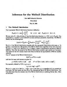
The model took for generating coherent Weibull sequences is shown in fig. 1. This generator is composed of two blocks. The first one is the Correlator Filter, which is used to correlate a coherent white Gaussian sequence (CWGS), in order to obtain a coherent correlated Gaussian sequence (CCGS). This block is explained in depth in the subsection 3.1. The second block is used to obtain the coherent correlated Weibull sequence (CCWS) from a CCGS with an specified covariance matrix. This block is explained in depth in the subsection 3.2.
Correlator filter
The aim of this block is to obtain a CCGS with a desired covariance matrix from a zero mean and unity power CWGS. This covariance matrix involves parameters like the correlation coefficient of the samples and the power of the sequence. This matrix, its properties and the way to obtain it are explained in depth in the subsection 3.2. The first step to achieve our objective is to generate a CWGS. This sequence is obtained with (6). ξ 0 [k] = x0 [k] + jy 0 [k]
(6)
where k denotes the k-th instant of the sequence and the sequences x0 and y 0 are real-valued gaussian sequences with zero mean and a power of √12 , each. So the sequence ξ 0 has zero mean and unity power. In order to transform the CWGS present at the input of the Correlator Filter in the desired CCGS , it is necessary to obtain the coefficients of this filter. The filter makes the transformation of the sequences like is noted in (7) 1
ξ = U ∗L 2 ξ0
(7)
where U is the matrix with the eigenvectors of the covariance matrix of the desired CCGS (McG ) and L is the diagonal matrix with the eigenvectors of the McG matrix. The sizes of both matrixes is N xN , where N is the length of the sequence (column vector) of ξ and ξ0.
3.2
NonLinear MemoryLess Transformation
This block deals with the problem to obtain a CCWS with a desired covariance matrix (McW ) from a CCGS. In order to design it, it is necessary to define which are the parameters of the CCWS and its covariance matrix (McW ). One way to obtain a CCWS from a CCGS is shown in fig. 2 [5] . In this figure, a denotes the skewness parameter of a Weibull sequence. It is demonstrated in [2] that the McW matrix depends on the power of the CCWS (PcW ), the correlation coefficient of the CCWS (ρcW ) and its doppler
Proceedings of the 5th WSEAS Int. Conf. on Signal Processing, Robotics and Automation, Madrid, Spain, February 15-17, 2006 (pp376-380)
Re{x [k ]} x [k ] Im{x [k ]}
x[k ]
y[k ]
u[k ]
(·)2
X
( ·)
+
1 1 a 2
+
v[k ]
(·)
2
X
w[k ]
j
Figure 2: NonLinear MemoryLess Transformation (NLMLT) frequency (fcW ). The last parameter is an application of the problem we deal with, the generation of synthetic radar sequences. Expression (8) shows how the McW matrix is computed knowing these parameters of the sequence. (McW )h,k =
|h−k| PcW ρcW ej(2π(h−k)fcW )
(8)
where Γ() is the Eulero Gamma function [7] and F (A; B; C; D) is the Gauss Hypergeometric function [7], b is the scale parameter (related with the power of the sequence) and a is the shape parameter (called skewness parameter) of the Weibull sequence. It is appreciated that for a = 2, the correlation coefficients ρcW and ρcG are the same because the sequences at the input (ξ) and at the output (w) coincide. This affirmation can be compared with that obtained in the section 2 for the same value of a. In [5] it is demonstrated that for high values of ρcG , a linear dependency between ρcW and ρcG can be drawn by (13) ρcW = Ka ρcG + (1 − Ka )
(13)
where Ka depends on the value of the skewness parameter of the Weibull sequence. A set of Ka values is given in (14)
In (8), h and k denote the indexes of the elements of the matrix, where both varies from 1 to N (length of the sequence to generate). Whereas, the McG matrix is computed with expression (9) in the same way as (8) and with the same kind of parameters but applied to the CCGS, where h and k are the same as used in (8).
K0.6 = 1.758 K0.8 = 1.406 K1.2 = 1.112
4
(14)
(9)
Confidence of the generated sequences
For the expressions (8) and (9), several relationships between their parameters exist. The power of the CCGS (PcG ) is related to the power of the CCWS (PcW ) using the expression (10). The PcW depends only of the a and b parameters of the CCCWS. These parameters, its use and its interpretation are defined for expression (12).
The confidence of the generated sequences is measured in two ways, based in the Probability Distribution Function (PDF) and based in the covariance matrix. The first one deals with the mean error obtained in the PDF between the theoretical and practical cases. This error is measured with the expression (15)
|h−k| j(2π(h−k)fcG )
(McG )h,k = PcG ρcG
e
PcG = ba
(10)
The doppler frequency of the CCGS (fcG ) is related to the doppler frequency of the CCWS (fcW ) using the expression (11). fcG = fcW
(11)
The relationship between the correlation coefficient of the CCWS (ρcW ) and the coefficient of the CCGS (ρcG ) is given by (12) µ
ρcW
´ 2 +1 1 3 ρcG a ³ a 2 + Γ2 1 − ρ = cG 2 a 2 aΓ( a ) ¶ µ 1 3 1 3 + ; + ; 2; ρ2cG F a 2 a 2
(12)
eP DF =
M 1 X |P DFT H − P DFP R | M k=1
(15)
where M is the number of bins took for the discretization of the theoretical PDF (P DFT H ) and the practical PDF (P DFP R ). The P DFT H is the theoretical PDF of a Weibull sequence with specific a and b parameters. Whereas, the P DFP R is estimated with the histogram of M bins of the generated sequence obtained from the generator proposed in section 3. The second way to measure the confidence of the generated sequence is based in the computation of the mean error of the covariance matrix generated by the generator proposed in section 3. This error can be calculated with expression (16)
Proceedings of the 5th WSEAS Int. Conf. on Signal Processing, Robotics and Automation, Madrid, Spain, February 15-17, 2006 (pp376-380)
p =0.8 cw
a=0.6
b=3.3
pcw=0.9
P =20dB cw
a=0.6
b=3.3
Pcw=20dB
50
50 40
40
30
30
20
20
10
10 0
50
100
150
200 250 Index of the sequence (k)
pcw=0.8
a=1.2
b=8.3
300
350
0
400
50
100
150
200 250 Index of the sequence (k)
pcw=0.9
Pcw=20dB
a=1.2
b=8.3
300
350
400
300
350
400
Pcw=20dB
50
50 40
40
30
30
20
20
10
10 0
50
100
150
200 250 Index of the sequence (k)
300
350
0
400
Figure 3: Temporal representation of the discrete time Weibull sequence for the same Clutter Power (Pcw = 20dB) and different combination of parameters like {ρcw = 0.8; a = 0.6; b = 3.3} and {ρcw = 0.8; a = 1.2; b = 8.3}
eMc
1 = 2 N
¯N N ¯ ¯X X ¡ 0 ¢ ¯¯ ¯ (Mc )h,k − Mc h,k ¯ ¯ ¯ ¯
(16)
k=1 n=1
where ()h,k denotes the indexes of the element the matrixes Mc (the desired covariance matrix of the sequence) and Mc0 (the covariance matrix of the generated sequence). The matrix Mc0 can be obtained with the expression (17) Mc0 = E[w∗ wT ]
(17)
where E[] is the mathematical expectation, w∗ denotes the complex conjugation of the samples that compose the coherent Weibull sequence w and wT denotes the transposition of the matrix (vector) where is stored the coherent Weibull sequence w.
5
Results
According to the explanations of the previous sections, here it is shown the results of the analysis of the generated sequences. Figures 3 and 4 show the temporal representation of several Weibull sequences generated with the model we propose. They are generated for coefficient parameters usually used in the generation of radar models [5]. These values of the parameters are ρcW = 0.8 and ρcW = 0.9, which indicates that the samples of the sequences have a high correlation between them. This effect is perfectly viewed in both figures. The length of the sequences generated is 1000
50
100
150
200 250 Index of the sequence (k)
Figure 4: Temporal representation of the discrete time Weibull sequence for the same Clutter Power (Pcw = 20dB) and different combination of parameters like {ρcw = 0.9; a = 0.6; b = 3.3} and {ρcw = 0.9; a = 1.2; b = 8.3} samples, but in the figures is only represented the first 400 samples in order to view it with more detail. In figures 5 and 6 it is shown the theoretical and practical (measured with the histogram) PDFs. As can be observed in both examples, the practical and theoretical PDFs are very similar. This test was made for different values and the PDFs were always very close. So, it can be conclude that the model proposed approximate the Weibull distribution for different combination of parameters. Moreover, the phase distribution of the generated Weibull sequences is uniform, as was taken in the model. This affirmation is made taking into account the results shown in fig. 7. The confidence, based in the PDF error, of the generated sequences gives the following results: eP DF = 2.0e−3 for parameters {ρcw = 0.9; a = 0.6; b = 3.3; Pcw = 20dB} and eP DF = 5.2e−3 for parameters {ρcw = 0.9; a = 1.2; b = 8.3; Pcw = 20dB}. This errors have been obtained as the mean of several trials. Whereas the confidence based on the covariance matrix error of the generated Weibull sequences is: eMc = 0.117 for parameters {ρcw = 0.9; a = 0.6; b = 3.3; Pcw = 20dB} and eMc = 0.106 for parameters {ρcw = 0.9; a = 1.2; b = 8.3; Pcw = 20dB}. Both errors are very low, so the generated sequences can be taken as correct coherent Weibull sequences.
6 Conclusions As can be observed in the results obtained for the generated sequences, several signs avoid us to think that the model proposed approximate the Weibull distrib-
Proceedings of the 5th WSEAS Int. Conf. on Signal Processing, Robotics and Automation, Madrid, Spain, February 15-17, 2006 (pp376-380)
PDFs of the theoretical and practical Weibull sequence (|w|) for pcw=0.9;a=0.6;b=3.3;Pcw=20dB
PDFs of the theoretical and practical Weibull sequence (|w|) for pcw=0.9;a=1.2;b=8.3;Pcw=20dB
0.4
0.12 Theoretical PDF Practical PDF
Theoretical PDF Practical PDF
0.1
0.3 PDF
PDF
0.08 0.2
0.06 0.04
0.1 0.02 0
0
10
20
30
40
50 |w|
0.25
60
70
80
90
0
100
0
5
10
15
20 |w|
25
0.1
0.1
0.1
0.08
0.08
0.08
0.06
0.06
0.06
30
35
40
0.1 0.05 0
5
10 |w|
15
PDF
PDF
PDF
PDF
0.2 0.15
0.04
0.04
0.04
0.02
0.02
0.02
0
20
40
60
80
0
2
|w|
Figure 5: Theoretical and Practical PDFs for a discrete time Weibull sequence of parameters {ρcw = 0.9; a = 0.6; b = 3.3; Pcw = 20dB} ution we are looking forward. The first sign is that the distribution of the modulus of the coherent sequence is approximated in a correct way by the model proposed. The second sign is that the phase distribution of the coherent sequence has a circular symmetry in the Real Vs Imaginary part representation, what is an indicative that its phase distribution is uniform. And the third one is that the coefficients (errors) took for estimating the confidence of the generated sequences are very low, what is an indication that the model works. References: [1] F. Gini, F. Lombardini and L. Verrazzani, ”Decentralized CFAR detection with binary integration in Weibull clutter”, IEE Trans. on Aerospace and Electronic Systems, vol. 33, NO. 2, April 1997, pp. 396-407. [2] V. ALOISIO, A. DI VITO and G. GALATI, ”Optimum detection of moderately fluctuating radar targets”, IEE Proc. on Radar, Sonar and Navigation, vol. 141, NO. 3, June 1994, pp. 164170. [3] K. Cheikh and S. Faozi, ”Application of neural networks to radar signal detection in Kdistributed clutter”, First International Symposium on Control, Communications and Signal Processing Workshop Proceedings, 18-21 July 2004, pp. 633-637. [4] D. C. Schleher, Automatic detection and radar data processing, Artech House, 1980. [5] A. Farina, A. Russo, F. Scannapieco and S. Barbarossa, ”Theory of radar detection in coherent
4 |w|
0
6
10
15
20
25 |w|
30
35
Figure 6: Theoretical and Practical PDFs for a discrete time Weibull sequence of parameters {ρcw = 0.9; a = 1.2; b = 8.3; Pcw = 20dB} 40 30 20 10 0 −10 −20 −30 −40 −40
−30
−20
−10
0
10
20
30
40
Figure 7: Real Vs Imaginary parts of discrete time Weibull sequence of parameters {ρcw = 0.9; a = 0.6; b = 3.3; Pcw = 20dB}. Demonstration that its phase have a circular (uniform) distribution Weibull clutter”, in Optimised Radar Processors, IEE Radar, Sonar, Navigation and Avionics Series 1, Peter Peregrinus Ltd., London, UK, 1987, pp. 100-116. [6] A. Farina, A. Russo and F. Scannapieco, ”Radar detection in coherent Weibull clutter”, IEEE Trans. on Acoustics, Speech and Signal Processing, vol. ASSP-35, NO. 6, June 1987, pp. 893895. [7] I. S. Gradshteyn and I. M. Ryzhik, Table of integrals, series ans products, Academic Press, 1965.