modern coding theory

MODERN CODING THEORY

Preliminary version – January 24, 2007


Modern Coding Theory BY

T. R I C H A R D S O N A N D R . U R B A N K E

Cambridge University Press


Modern Coding Theory Copyright ©2006 by T. Richardson and R. Urbanke All rights reserved Library of Congress Catalog Card Number: 00–00000 isbn 0-000-00000-0


WA R N I N G — U S E A T O W N R I S K These notes are work in progress and change daily. The most current version can be found at . Although we are not bold (nor rich) enough to offer a monetary award for typos found, we would greatly appreciate any feedback.

v Preliminary version – January 24, 2007


P R E FA C E This book is an attempt to summarize the state-of-the-art of iterative coding. Two other popular names which describe the same area are probabilistic coding and codes on graphs. Originally devised by Gallager in 1961 in his remarkable thesis, then long forgotten, and rediscovered by Berrou, Glavieux and Thitimajshima in 1993, iterative techniques have had a strong impact on coding theory and practice and, more generally, on the whole of communications. The title Modern Coding Theory is clearly preposterous. After all, there have been several other important recent developments in coding theory. To name just the most prominent one, Sudan’s list decoding algorithm for Reed-Solomon codes and its extension to soft-decision decoding have sparked new life in what was considered a fairly mature subject. So what is our excuse? We simply could not resist. But the font on the book cover is supposed to express the irony that the roots of “modern” coding go back to a time when typewriters ruled the world. This book is written with several audiences in mind. We hope that it will be a useful source for a course in coding theory. If such a course is dedicated solely to iterative techniques, most necessary material should be contained in this book. If the course covers both classical and iterative topics, this book can be used in conjunction with one of the many excellent books on classical coding. We have excluded all classical material on purpose, except for the most basic definitions. We hope that this book will also be of use to the practitioner in the field who is trying to decide what coding scheme to employ, how a new scheme can be designed, or how an existing system can be improved. It is important to note that the field of iterative coding has not settled in the same way as classical coding has. There are as many flavors of iterative coding systems – and graphical models to denote them – as there are researchers in the field. We have therefore decided to focus more on techniques to analyze and design such systems rather than specific such instances. In order to present the theory we have chosen Gallager’s original ensemble of low-density parity-check codes as a representative example. This ensemble is simple enough that the main results can be presented easily. Once the basic concepts are absorbed, their extension to more general cases is typically routine and several (but not an exhaustive list) of such extensions are discussed. In particular, we have included a thorough investigation of turbo-codes. Another characteristic of this book is that we spend a considerable number of pages on discussing iterative coding over the binary erasure channel. Why spend so much time on a very specific and limited channel model? It is probably fair to say that all we know about iterative coding we learned first for the binary erasure channel. vii Preliminary version – January 24, 2007

viii

preface

Due to the special properties of this channel, its analysis needs not much more than pen and paper and some basic knowledge of calculus and probability. All important concepts encountered during the study of the binary erasure channel seem to carry over to general channels, although our ability to prove some of these extensions is frequently dwarfed by technical challenges. There are many possible paths through this book. Our own personal preference is to cover the core of the material in Chapter 3 (binary erasure channel) and Chapter 4 (general channels) in a linear fashion. The remaining material can be read in almost any order according to the preferences of the reader. E.g., at this point it might be rewarding to broaden the view and to go through some of the material on factor graphs and its applications (Chapter 2). Alternatively, the reader might be more interested in exploring other ensembles, e.g., the class of turbo codes discussed in Chapter 5 or multi-edge ensembles in Chapter 7. It is also possible to take the chapter on factor graphs (Chapter 2) as a starting point, reviewing some of the basic definitions along the way, and to return to the more detailed analysis later. The material covered in this chapter has the special appeal that it unifies many themes of information theory, coding, and communication theory. Although all three areas trace their origin to Shannon’s 1948 paper, they have subsequently diverged to a point where a typical textbook in one area treats each of the other two topics at most in passing. The factor graph approach is a nice way to glue them back together. One and the same technique allows for the computation of capacity, and deals with equalization, modulation and coding on an equal footing. Chapter 7 deals with various ensembles and the issues of graph designs. We have not tried to give an exhaustive list of all known iterative codes since this list is growing daily and there is no sign that this growth will stop anytime soon. Rather, we have tried to pick some representative examples. Chapter 8 gives a brief look at a complementary way of analyzing iterative systems in terms of the expansion of the underlying bipartite graph. The Appendix contains various chapters on topics which either describe tools for analysis or are simply too technical to fit into the main part. Chapter A takes a look at the encoding problem. Curiously, for iterative schemes the encoding task can be of equal complexity (or even higher) than the decoding task. Appendix B discusses efficient and accurate ways of implementing density evolution. In Appendix C we describe various techniques from probability which are useful in asserting that most elements of a properly chosen ensemble behave “close” to the ensemble average. We take a close look at generating functions in Appendix D In particular we discuss how to accurately estimate the coefficients of powers of polynomials – a recurrent theme in this book. Although we have tried to make the material as accessible as possible, the prerequisites for various portions of the book vary considerably. Some seemingly simple


ix questions need quite sophisticated tools for their answer. A good example is the material related to the weight distribution of LDPC codes and their error floor behavior. In these cases, when the density of equations increases to a painful level, the casual reader is advised not to get discouraged but rather to skip the proofs. Fortunately, in all these cases the subsequent material depends very little on the mathematical details of the proof. We started out to write a thin book containing all there is to know about iterative coding. We ended up with a rather thick one and a number of regrettable omissions. To mention just the most important ones: we do not cover the emerging theory of pseudo codewords and their connections to the error floor for general channels. We only scratched the surface of the rich area of interleaver design. Rateless codes deserve a much more prominent role, and there is no discussion of the powerful techniques borrowed from statistical mechanics which have been used successfully in the analysis. But rather than ending with regrets, let us close with the following (slightly modified) quote by Descartes: “[We] hope that posterity will judge [us] kindly, not only as to the things which [we] have explained, but also as to those which [we] have intentionally omitted so as to leave to others the pleasure of discovery.” ;-) HERE GO ACKNOWLEDGMENTS. T. Richardson Richardson’s Island


R. Urbanke Lausanne September 1, 2020


CONTENTS WARNING — use at own risk ċ page v Preface ċ page vii 1

Introduction ċ page 1 §1.1 Codes and their Applications ċ 1 §1.2 Communications Problem ċ 1 §1.3 Coding: Trial and Error ċ 3 §1.4 Codes and Ensembles ċ 5 §1.5 MAP and ML Decoding ċ 7 §1.6 Channel Coding Theorem ċ 8 §1.7 Linear Codes and Their Complexity ċ 11 §1.8 Rate, Probability, Complexity, and Length ċ 17 §1.9 First Tour of Iterative Coding ċ 21 §1.10 Notation, Conventions, and Some Useful Facts ċ 26 Notes ċ 30 Problems ċ 32 References ċ 40

2

Factor Graphs ċ page 45 §2.1 Distributive Law ċ 45 §2.2 Graphical Representation of Factorizations ċ 46 §2.3 Recursive Determination of Marginals ċ 47 §2.4 Efficient Marginalization Via Message Passing ċ 50 §2.5 Decoding via Message Passing ċ 52 §2.6 Limitations of Cycle-Free Codes ċ 59 §2.7 Message-Passing on Codes with Cycles ċ 60 Notes ċ 61 Problems ċ 62 References ċ 63

3

Binary Erasure Channel ċ page 67 §3.1 Channel Model ċ 67 §3.2 Transmission via Linear Codes ċ 68 §3.3 Tanner Graphs ċ 71 §3.4 Low-Density Parity-Check Codes ċ 73 xi Preliminary version – January 24, 2007

xii

contents §3.5 Message-Passing Decoder ċ 78 §3.6 Two Basic Simplifications ċ 80 §3.7 Computation Graph and Tree Ensemble ċ 84 §3.8 Tree Channel and Convergence to Tree Channel ċ 90 §3.9 Density Evolution ċ 91 §3.10 Monotonicity ċ 92 §3.11 Threshold ċ 94 §3.12 Fixed Point Characterization of Threshold ċ 95 §3.13 Stability ċ 96 §3.14 EXIT Chart ċ 97 §3.15 Capacity-Achieving Degree Distributions ċ 104 §3.16 Gallager’s Lower Bound on the Density ċ 107 §3.17 Optimally-Sparse Degree Distribution Pairs ċ 110 §3.18 Degree Distributions with Given Maximum Degree ċ 111 §3.19 Peeling Decoder and Order of Limits ċ 113 §3.20 EXIT Function and MAP Performance ċ 118 §3.21 Maxwell Decoder ċ 128 §3.22 Exact Finite-Length Analysis ċ 131 §3.23 Finite-Length Scaling ċ 140 §3.24 Weight Distribution and Error Floor ċ 145 Notes ċ 152 Problems ċ 156 References ċ 164

4

Binary Memoryless Symmetric Channels ċ page 169 §4.1 Basic Definitions and Examples ċ 169 §4.2 Message-Passing Decoder ċ 206 §4.3 Two Basic Simplifications ċ 212 §4.4 Tree Channel and Convergence to Tree Channel ċ 214 §4.5 Density Evolution ċ 214 §4.6 Monotonicity ċ 218 §4.7 Threshold ċ 222 §4.8 Fixed Point Characterization of Threshold ċ 222 §4.9 Stability ċ 226 §4.10 EXIT Chart ċ 234 §4.11 Gallager’s Lower Bound on the Density ċ 244 §4.12 GEXIT Function and MAP Performance ċ 248 §4.13 Finite-Length Scaling ċ 263 §4.14 Error Floor under MAP Decoding ċ 264 Notes ċ 265


xiii Problems ċ 270 References ċ 284 5

Convolutional Codes and Turbo Codes ċ page 291 §5.1 Convolutional Codes ċ 291 §5.2 Turbo Codes: Structure and Encoding ċ 300 §5.3 Turbo Codes: Decoding ċ 303 §5.4 Turbo Codes: Symmetry, All-One Codeword Assumption, Concentration, and Computation Graph ċ 306 §5.5 Turbo Codes: Density Evolution ċ 307 §5.6 Turbo Codes: Stability Condition ċ 311 §5.7 Turbo Codes: EXIT Chart ċ 313 §5.8 Turbo Codes: GEXIT Function and MAP Performance ċ 314 §5.9 Weight Distribution and Error Floor ċ 315 §5.10 Turbo Codes: Variations on the Theme ċ 329 Notes ċ 332 Problems ċ 336 References ċ 340

6 General Channels ċ page 347 §6.1 Fading Channel ċ 347 §6.2 Z Channel ċ 350 §6.3 Channels with Memory ċ 353 §6.4 Coding for High Spectral Efficiency ċ 360 §6.5 Multiple-Access Channel ċ 363 Notes ċ 367 Problems ċ 369 References ċ 372 7

General Ensembles ċ page 379 §7.1 Multi-Edge Type LDPC Ensembles: Definition ċ 380 §7.2 Multi-Edge Type LDPC Ensembles: Analysis ċ 387 §7.3 Structured Graphs ċ 397 §7.4 Non-Binary Codes ċ 404 §7.5 Low-Density Generator Codes and Rate-Less Codes ċ 409 Notes ċ 416 Problems ċ 419 References ċ 420


xiv 8

contents Expander Codes and the Flipping Algorithm ċ page 425 §8.1 Building Codes from Expanders ċ 425 §8.2 Flipping Algorithm ċ 426 §8.3 Bound on the Expansion of a Graph ċ 427 §8.4 Expansion of a Random Graph ċ 429 Notes ċ 431 Problems ċ 432 References ċ 432

A Encoding Low-Density Parity-Check Codes ċ page 433 §A.1 Encoding Generic LDPC Codes ċ 433 §A.2 Greedy Upper Triangulation ċ 439 §A.3 Linear Encoding Complexity ċ 444 §A.4 Analysis of Asymptotic Gap ċ 447 Notes ċ 452 Problems ċ 452 References ċ 453 B Efficient Implementation of Density Evolution ċ page 455 §B.1 Quantization ċ 456 §B.2 Variable Node Update Via Fourier Transform ċ 456 §B.3 Check-Node Update Via Table Method ċ 458 Notes ċ 460 Problems ċ 461 References ċ 461 C Concentration Inequalities ċ page 463 §C.1 First and Second Moment Method ċ 464 §C.2 Bernstein Inequality ċ 466 §C.3 Martingales ċ 468 §C.4 Wormald’s Differential Equation Approach ċ 474 §C.5 Convergence to Poisson Distribution ċ 480 Notes ċ 483 Problems ċ 484 References ċ 485 D Formal Power Sums ċ page 487 §D.1 Definition ċ 487 §D.2 Basic Properties ċ 487 §D.3 Summation of Subsequence ċ 488


xv §D.4 Coefficient Growth of Powers of Polynomials ċ 489 §D.5 Unimodality ċ 505 Notes ċ 506 Problems ċ 507 References ċ 511



Chapter 1

INTRODUCTION §1.1. Codes and their Applications Codes play an important role in many areas of science. To name just a few: in mathematics they give rise to dense lattices and allow the construction of designs for use in statistics. In the area of computer science, public-key crypto systems may be based on codes, they are the crucial ingredient for some extractors – generating many weakly random bits from a few truly random ones – and they make efficient hashing functions. Codes are helpful in minimizing the communication complexity and they can be used to turn worst-case hardness into average-case hardness. In the area of communications, codes help to represent sources efficiently, to combat the noise introduced by the communication channel, to avoid large peak-to-average power ratios, or to minimize interference in multi-user systems. It should not come as a surprise that different properties of codes are relevant for the diverse applications mentioned above. The covering radius of a code is important for the source coding problem whereas its minimum distance is of interest for secret-sharing applications. Maximum-distance separable codes are useful for pseudorandom generators, and the algorithmic aspects of the decoding problem are called for when using codes as an ingredient of a public-key crypto system. In this book we consider codes exclusively for their suitability for the channel coding problem: we want to transmit a message across a noisy channel so that the receiver can determine this message with high probability despite the imperfections of the channel. We are interested in low-complexity schemes that introduce little delay and allow reliable transmission close to the ultimate limit, the Shannon capacity.

§1.2. Communications Problem Let us review the simplest communications scenario – the point-to-point communications problem depicted in Figure 1.1. A source (speech, audio, data, . . . ) transmits source

channel

sink

Figure 1.1: The basic point-to-point communications problem. via a noisy channel (phone line, optical link, wireless, storage medium, . . . ) to a sink. We are interested in reliable transmission, i.e., we want to recreate the transmitted 1 Preliminary version – January 24, 2007

2

introduction

information with as little distortion (number of wrong bits, mean squared error distortion, . . . ) as possible at the sink. In his seminal paper in 1948, Shannon formalized the above problem and showed that the point-to-point problem can always be decomposed into two separate problems as shown in Figure 1.2. First, the source encoder transforms the source into a bit stream. Ideally, the source encoder removes all redundancy from the source so that the resulting bit stream uses the smallest possible number of bits while still representing the source with sufficient accuracy. The channel encoder then processes the bit stream to add redundancy. This redundancy is carefully chosen so as to combat the noise that is introduced by the channel. To be mathematically more precise: we model the output of the source as a stochastic process. For example, we might represent text as the output of a Markov chain, describing the local dependency structure of letter sequences. It is the task of the source encoder to represent this output as efficiently as possible (using as few bits as possible) given a desired upper bound on the distortion. The distortion measure is chosen by the user and is supposed to reflect the “cost” of deviating from the original source output. If the source emits points in Rn it might be natural to consider the squared Euclidean distance, whereas if the source emits binary strings a more natural measure might be to count the number of positions in which the source output and the word that can be reconstructed from the encoded source differ. Shannon’s source coding theorem asserts that, for a given source and distortion measure, there exists a minimum rate R = R(d) (bits per emitted source symbol) which is necessary (and sufficient) to describe this source with distortion not exceeding d. The plot of this rate R as a function of the distortion d is usually called the rate-distortion curve. In the second stage an appropriate amount of redundancy is added to these source bits to protect them against the errors in the channel. This process is called channel coding. Throughout the book we model the channel as a probabilistic mapping and we are typically interested in the average performance, where the average is taken over all channel realizations. Shannon’s channel coding theorem asserts the existence of a maximum rate (bits per channel use) at which information can be transmitted reliably, i.e., with vanishing probability of error, over a given channel. This maximum rate is called the capacity of the channel and is denoted by C. At the receiver we first decode the received bits to determine the transmitted information. We then use the decoded bits to reconstruct the source at the receiver. Shannon’s source-channel separation theorem asserts that the source can be reconstructed with a distortion of at most d at the receiver if R(d) < C, i.e., if the rate required to represent the given source with the allowed distortion is smaller than the capacity of the channel. Conversely, no scheme can do better. One great benefit of the separation theorem is that a communications link can be used for a large variety of sources: one good channel coding solution can be used with virtually any source. Virtually


coding: trial and error

3

all systems in use today are based on this principle. It is important though to be source

sink

source encoder

source decoder

channel encoder

channel decoder

channel

Figure 1.2: The basic point-to-point communications problem in view of the sourcechannel separation theorem. aware of the limitations of the source-channel separation theorem. The optimality is only in terms of the achievable distortion when large blocks of data are encoded together. Joint schemes might be substantially better in terms of complexity or delay. Also, the separation is no longer valid if one looks at multi-user scenarios. We will not be concerned with the source coding problem or, equivalently, we assume that the source coding problem has been optimally solved. For us, the source emits a sequence of independent identically distributed (iid) bits which are equally likely to be zero or one. Under this assumption, we will see how to accomplish the channel coding problem in an efficient manner for a variety of scenarios.

§1.3. Coding: Trial and Error How can we transmit information reliably over a noisy channel at a strictly positive rate? At some level we have already given the answer: add redundancy to the message that can be exploited to combat the distortion introduced by the channel. By starting with a special case we want to clarify the key concepts. 1

1−є

1

xt

є є

Yt

-1

1−є

-1

Figure 1.4: BSC(є) Example 1.3 (Binary Symmetric Channel). Let us introduce the binary symmetric channel with cross-over probability є depicted in Figure 1.4. We denote it by


4

introduction

BSC(є). Both input x t and output Yt are elements of 1. (As explained in more detail in Section 1.10, we write the input in lower case, since it might be fixed, but we write the output in upper case, since it is always a random variable.) A transmitted bit is either received correctly or received flipped, the latter occurring with probability є, and different bits are flipped or not flipped independently. Without loss of generality we can assume that 0 < є < 12 . The BSC is the generic model of a binary memoryless channel in which hard decisions are made at the front end of the receiver, i.e., where the received value is quantized to two values. First Trial: we start by considering uncoded transmission over the BSC(є). Thus, we send the source bits across the channel as is, without the insertion of redundant bits. At the receiver we estimate the transmitted bit X based on the observation Y. As we will learn soon in Section 1.5, the optimal decision rule, call it xˆ MAP (y), is to choose that x 1 which maximizes p X Y (x y) for the given y. For the given case this estimator reduces to xˆ MAP (y) = y. The probability that the estimate differs from the true value, i.e., Pb P xˆMAP (Y) X, is equal to є. Since for every information bit we want to convey we send exactly one bit over the channel we say that this scheme has rate 1. We conclude that with uncoded transmission we can achieve a (rate, Pb )-pair of (1, є). Second Trial: if this error probability is too high for our application, what transmission strategy can we use to lower it? The simplest strategy is repetition-coding. Assume we repeat each bit k times. To keep things simple, assume that k is odd. So if X, the bit to be transmitted, has value x then the input to the BSC(є) is the k-tuple x, , x. Denote the k associated observations by Y1 Yk . It is not hard to see that the optimal estimator is given by the majority rule xˆMAP (y1 , , y k ) = majority of y1 , , y k . Hence the probability of bit error is given by k k odd Pb = P xˆ MAP (Y) X = Pat least k2 errors occur = є i (1 − є)k−i . ik2 i Since for every information bit we want to convey we send k bits over the channel we say that such a scheme has rate 1k . So with repetition codes we can achieve the (rate, Pb )-pairs ( 1k , ik2 kiє i (1 − є)k−i ). For Pb to approach zero we have to choose k larger and larger and as a consequence the rate approaches zero as well. Can we keep the rate positive and still make the error probability go to zero?


codes and ensembles

5

§1.4. Codes and Ensembles Definition 1.5 (Code). A code C of length n and cardinality M over a field F is a subset of Fn with M elements, i.e., C(n, M) x [1] , , x [M] , x [i] Fn , 1 i M. The elements of the code are called codewords. The parameter n is called the blocklength. Example 1.6 (Repetition Code). Let F = F2 , the binary field consisting of 0, 1 with the operations and . We write + for and ċ for (0 + 0 = 1 + 1 = 0; 0 + 1 = 1; 0 ċ 0 = 1 ċ 0 = 0; 1 ċ 1 = 1). The repetition code is defined as C(n = 3, M = 2) = 000, 111. Definition 1.7 (Rate). The rate (measured as information symbols per transmitted symbol) of a code C(n, M) is r n1 log F M. Example 1.8 (Repetition Code). Let F = F2 . We have r(C(3, 2)) = It takes 3 channel symbols to transmit one information symbol.

1 3

log2 2 = 13 .

The following two definitions will play a role only much later in the book. But it is convenient to collect them here for reference. Definition 1.9 (Support Set). The support set of a codeword x C is the set of locations i [n] = 1, , n such that x i 0. Definition 1.10 (Minimal Codewords). Consider a binary code C, i.e., a code over F2 . We say that a codeword x C is minimal if its support set does not contain the support set of any other (non-zero) codeword. Definition 1.11 (Hammming Weight and Hamming Distance). Let u, v Fn . The Hamming weight of a word u, which we denote by w(u), is equal to the number of non-zero symbols in u, i.e., the cardinality of the support set. The Hamming distance of a pair (u, v), which we denote by d(u, v), is the number of positions in which u differs from v. We have d(u, v) = d(u − v, 0) = w(u − v). Further, d(u, v) = d(v, u) and d(u, v) 0, with equality if and only if u = v. Also, d(ċ, ċ) fulfills the triangle inequality d(u, v) d(u, t) + d(t, v), for any triple u, v, t Fn . In words, d(ċ, ċ) is a true distance in the mathematical sense.


6

introduction

Definition 1.12 (Minimum Distance of a Code). Let C be a code. Its minimum distance d(C) is defined as d(C) min d(u, v) u, v C, u v .

Let x Fn and t N. A sphere of radius t centered at the point x is the set of all points in Fn that have distance at most t from x. If, for a code C of minimum around each codeword, then these distance d, we place spheres of radius t d−1 2 spheres are disjoint. This follows from the triangle inequality. Further, by definition of d, t is the largest such radius. The radius t has an important operational meaning that explains why much of classical coding is centered on the construction of codes with large minimum distance. To be concrete, consider the binary case. Assume we use a code C(n, M, d) (i.e., a code with M codewords of length n and minimum distance d) for transmission over a BSC and assume that we employ a bounded distance decoder with decoding radius t. More precisely, given y the decoder chooses xˆBD (y) defined by x C, xˆBD (y) error,

if d(x, y) t and d(x , y) otherwise,

t, ∀x C " x,

δ (r)

where by “error” the decoder declares that it is unable to decode. Such a combination corrects all errors of weight t or less. Therefore, a large t implies a large resilience against channel errors.

0.3 0.2 0.1 0.0

0.2 0.4 0.6 0.8

r

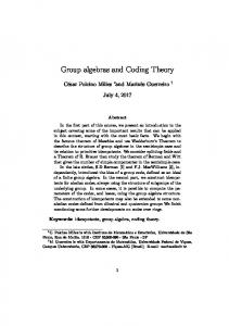
Figure 1.13: Upper and lower bound on δ (r). How large can d (and hence t) be made in the binary case? Let δ dn denote the normalized distance and consider for a fixed rate r, 0 < r < 1, δ (r) lim sup max # n

d(C) C C $n, 2nr %& . n

Problem 1.13 discusses the asymptotic Gilbert-Varshamov bound h2−1 (1 − r) δ (r),


map and ml decoding

7

where h2 (x) −x log2 x − (1 − x) log2 (1 − x) is the binary entropy function and where for y [0, 1], h2−1 (y) is the unique element x [0, 12 ] such that h2 (x) = y. There exists a related upper bound due to Elias which states that (1.14)

δ (r) 2h2−1 (1 − r)(1 − h2−1 (1 − r)).

Both bounds are illustrated in Figure 1.13. We can now answer the question posed at the end of the previous section. For a fixed channel BSC(є) pick a rate r such that δ (r) 2є+ω, where ω is some arbitrarily small but strictly positive quantity. We see from the Gilbert-Varshamov bound that such a strictly positive r and ω exist as long as є < 14. Further, in this case we can find a code of arbitrarily large blocklength n of rate at least r and with relative minimum distance at least δ = 2є + ω. By the Chebyshev inequality (see Lemma C.3 on page 464), for every desired strictly positive probability P there exists a positive constant c such that the number of errors which one encounters in a block of length ' n is at most nє+c n with probability P. Assume now we employ a bounded distance ' decoder. If we choose n sufficiently large so that nє + c n < δn2 = nє + nω2, then the bounded distance decoder succeeds with probability at least P. Since P can be chosen arbitrarily close to 1 we see that there exist codes which allow transmission at a positive rate with arbitrarily small probability of error. Constructing provably good codes, with almost any reasonable interpretation of “good” is difficult. A standard approach to show the existence of good codes is the probabilistic method: an ensemble C of codes is constructed using some random process and one proves that “good” codes occur with positive probability. Often the probability is close to 1. This approach, used already by Shannon in his 1948 landmark paper, simplifies the task enormously (at the cost of a less useful result). Definition 1.15 (Shannon’s Random Ensemble). Let the field F be fixed. Consider the following ensemble C(n, M) of codes of length n and cardinality M. There are nM degrees of freedom in choosing a code, one degree of freedom for each component of each codeword. The ensemble consists of all F nM possible codes of length n and cardinality M endowed with a uniform probability distribution. To sample from this ensemble proceed as follows. Pick the codewords x [1] , , x [M] [i] randomly by letting each component x j be an independently and uniformly chosen element of F. We will see that such a code is likely to be “good” for many purposes.

§1.5. MAP and ML Decoding Assume we transmit over a channel with input F and output space Y using a code C(n, M) = x [1] , , x [M] . Let the channel be specified by its transition probability


8

introduction

pY X (y x). The transmitter chooses the codeword X C(n, M) with probability p X (x). (In communications the idea is that the transmitter wants to transmit one of M messages and uses one codeword for each possible message.) This codeword is then transmitted over the channel. Let Y denote the observation at the output of the channel. To what codeword should Y be decoded? If we decode Y to xˆ (Y) C, then the probability that we have made an error is 1 − p X Y (xˆ (Y) y). Thus, to minimize the probability of error we should choose xˆ (Y) to maximize p X Y (xˆ (Y) y). The maximum a posteriori (MAP) decoding rule reads xˆMAP (y) argmaxx C p X Y (x y) by Bayes’s rule

p X (x) pY (y) = argmaxx C pY X (y x)p X (x).

= argmaxx C pY X (y x)

Ties can be broken in some arbitrary manner without affecting the error probability. As we indicated, this estimator minimizes the probability of (block) error PB P xˆ MAP (Y) X. If all codewords are equally likely, i.e., if p X is uniform, then xˆ MAP (y) = argmaxx C pY X (y x)p X (x) = argmaxx C pY X (y x) xˆML (y), where the right hand side represents the decoding rule of the maximum likelihood (ML) decoder. In words, for a uniform prior p X the MAP and the ML decoders are equivalent.

§1.6. Channel Coding Theorem We have already seen that transmission at a strictly positive rate and an arbitrarily small probability of error is possible. What is the largest rate at which we can achieve a vanishing probability of error? Let us now investigate this question for transmission over the BSC(є). We are interested in the scenario depicted in Figure 1.16. For a given binary code C(n, M) the transmitter chooses with uniform probability a codeword X C(n, M) and transmits this codeword over the channel BSC(є). The output of the channel is denoted by Y. At the receiver the decoder estimates the transmitted codeword given the observation Y using the MAP rule xˆMAP (y). How small can we make (C, є) P Xˆ MAP X for given paramethe incurred block error probability PMAP B MAP (C, є) over all choices of ters n and M? Let Pˆ B (n, M, є) be the minimum of PMAP B C C(n, M). Theorem 1.17 (Shannon’s Channel Coding Theorem). If 0 < r < 1 − h2 (є) then n MAP Pˆ B (n, 2rn , є) *, 0.


channel coding theorem X C(n, M) chosen uniformly

X

BSC(є)

Y

9 decoder

Figure 1.16: Transmission over the BSC(є). Proof. Pick a code C from C(n, 2rn ), the random ensemble introduced in Definition 1.15. Since the MAP decoder is hard to analyze weuse the following suboptimal decoder. For some fixed ∆, ∆ 0, define ρ = nє + 2nє(1 − є)∆. If x [i] is the only codeword such that d(y, x [i] ) ρ then decode y as x [i] – otherwise declare an error. For u, v 1n let f (u, v) # and define

0, if d(u, v) ρ, 1, if d(u, v) ρ,

g [i] (y) 1 − f (x [i] , y) + f (x [j] , y). j i

Note that g [i] (y) equals zero if x [i] is the only codeword such that d(y, x [i] ) [i] ρ and that it is at least one otherwise. Let PB denote the conditional block error [i] probability assuming that X = x [i] , i.e., PB = Pxˆ (Y) X.X = x [i] . [i]

PB (C, є) =

yg [i] (y)1

= y 1n

+

pY X [i] (y x [i] )

y 1n

pY X [i] (y x [i] )g [i] (y)

pY X [i] (y x [i] )[1 − f (x [i] , y)]

[i] [j] pY X [i] (y x ) f (x , y)

y 1n j i

= P /d(Y , x [i] )

ρ X [i] = x [i] 0 +

[i] [j] pY X [i] (y x ) f (x , y).

y 1n j i

Note that d(y, x [i] ) = w(y+x [i] ), where y+x [i] is the vector of channel errors (recall that over F2 addition and subtraction are the same). It follows that d(Y , x [i] ) is the sum of n independent Bernoulli random variables, call it Z. Then Z is a random variable with mean nє and variance nє(1 − є). Recall from above that ρ = nє + 2nє(1 − є)∆. Therefore, from Chebyshev’s inequality (see Lemma C.3 on page 464) we get P /Z − nє

nє(1 − є)∆ ∆ = . 2nє(1 − є)∆0 2nє(1 − є) 2


10

introduction

We have PB (C, є) =

1 M [i] ∆ 1 M [i] [j] PB (C, є) + p [i] (y x ) f (x , y). M i=1 2 M i=1 y 1n j i Y X

Let EC(n,M) [ċ] denote the expectation with respect to the ensemble C(n, M). We conclude that Pˆ B (n, M, є) EC(n,M) 1PB (C, є)2

∆ 1 M [i] [j] + E [i] [ j] 1pY X [i] (y X ) f (X , y)2 2 M i=1 y 1n j i X ,X

(a)

=

∆ 1 M [i] [j] + E [i] 1pY X [i] (y X )2 E X [ j] 1 f (X , y)2 2 M i=1 y 1n j i X ρ

n

=

∆ 1 M [i] k=0 k + E1pY X [i] (y X )2 n 2 M i=1 y 1n j i 2

=

n ∆ + (M − 1) k=0n k , 2 2

ρ

where in step (a) we used the fact that if we consider for i j the two associated codewords X [i] and X [j] as random variables then they are by construction (pairn nh 2 (mn) which is valid wise) independent. If we now use the estimate m k=0 k 2 for m n2 (see (1.60) and Problem 1.22) then as ρ n2 for sufficiently large n

2є(1−є) ∆ )) n∆ Pˆ B (n, M, є) + (M − 1)2−n(1−h 2 (є+ 2 2є(1−є) ∆ nr −n(1−h 2 (є+ )) n∆ +2 2 2 2є(1−є) ∆ )−r) n∆ = + 2−n(1−h 2 (є+ 2 ∆ for n large enough if r < 1 − h2 (є).

The above argument is valid for any ∆

0.

The above proof shows that there exist codes in C n, 2nr which permit reliable transmission over the BSC(є) up to a rate of 1 − h2 (є) bits per channel use. Actually, a much stronger statement is true, namely almost any code in the above ensemble can be used for transmission at vanishing probabilities of error. Although we do not prove this here, the converse is true as well. Any attempt to transmit at a rate higher than 1−h2 (є) must result in error probabilities bounded away from zero.


linear codes and their complexity

11

Indeed, one can show that the block error probability PB must tend to one for any sequence of codes of increasing blocklength and rate strictly above 1 − h2 (є). Therefore, 1−h2 (є) is a threshold value, separating what is achievable from what is not. It is called the Shannon capacity of the BSC(є) and we denote it by CBSC (є) = 1 − h2(є). Example 1.18 (Bounded Distance Decoder is Not Sufficient). Consider a code of rate r, r (0, 1). By the Elias bound (1.14) the normalized minimum distance δ(r) is upper bounded by δ(r) 2h2−1 (1 − r)(1 − h2−1 (1 − r)), so that h2−1 (1 − r)

1 $1 − 1 − 2δ(r)% , 2

for δ(r) (0, 12). From this we deduce the weaker bound h2−1 (1 − r) 12 δ(r)

2

1 2 δ(r)

+

which is easier to handle. If we transmit over the BSC(є) then the expected number of errors in a block of length n is nє. Further, for large n with high ' probability the actual number of errors is within O( n) of this expected number (see the previous proof on page 9). Therefore, if we employ a bounded distance decoder we need 12 δ(r) є. If we combine this with the previous bound we get

3−1 since then the right hand side h2−1 (1 − r) є + є2 . This is not possible if є 2 exceeds 12. It follows that such a bounded distance decoder can not be used for 3−1 1 3−1 reliable transmission over a BSC(є) if є ( 2 , 2 ). And for є (0, 2 ) we conclude that r < 1 − h2 (є + є2 ) < 1 − h2 (є) = CBSC (є), i.e., capacity can not be achieved as well.

§1.7. Linear Codes and Their Complexity By our remarks above, almost any code in C n, 2nr is suitable for reliable transmission at rates close to Shannon capacity at low error probability provided only that the length n is sufficiently large (we have limited the proof of the channel coding theorem to the BSC but this theorem applies in a much wider setting). So why not declare the coding problem solved and stop here? The answer is that Shannon’s theorem does not take into account the description, the encoding and the decoding complexity. First note that, without further restriction on the structure, already the description of a particular code quickly becomes impractical as n grows, since it requires n2nr bits. Hence, as a first step towards a reduction in complexity we restrict our attention to linear codes. §1.7.1. Linear Codes We say that a code C over a field F is linear if αx + α x C, ∀x, x C and ∀α, α F .


12

introduction

Equivalently, a code C over a field F is linear if αx − x C, ∀x, x C and ∀α F .

(1.19)

Choosing α = 0 in (1.19) shows that if x C then so is −x . Further, choosing α = 1 and x = x shows that the all-zero word is a codeword of any (non-empty) linear code. For a linear code C the minimum distance d(C) is equal to the minimum of the weight of all non-zero codewords, d(C) min w(x − x ) x, x C, x x = min w(x) x C " 0 . Since Fn is a vector space, condition (1.19) implies that a linear code is a subspace of Fn . As such, C has a dimension k, 0 k n, so that C contains F k codewords. In the sequel we denote by [n, k, d] the parameters of a linear code of length n, dimension k and minimum distance d. It is customary to call a k3n matrix G, whose rows form a linearly independent basis for C, a generator matrix for C. Conversely, given a matrix G Fkn we can associate with it the code C(G), (1.20)

C(G) x Fn x = uG, u Fk .

There are many generator matrices G which describe the same code (see Problem 1.5). Definition 1.21 (Proper Codes). We say that a linear code is proper if its generator matrix G has no zero columns.1 Zero columns convey zero information – no pun intended – and so we can safely restrict our attention to proper codes in the sequel. Definition 1.22 (Systematic Generator Matrix). A generator matrix G of a linear code C[n, k, d] is said to be in systematic form if G = (I k P), where I k is a k 3 k identity matrix and P is an arbitrary k 3 (n − k) matrix with entries in F. If G is in systematic form and u Fk is an information word, then the corresponding codeword x = uG has the form (u, uP), i.e., the first k components of x are equal to the information word u. To each linear code C we associate the dual code C , (1.23)

C w Fn xw T = 0, ∀x C = w Fn Gw T = 0T .

1

Note that properness is a code property. I.e., it does not depend on the generator matrix G which we choose to represent C.



13

Assume that w and w are elements of C and that x is an element of C. Since xw T = 0 = x(w )T implies x(αw − w )T = 0 for any α F, it follows that C is a linear code as well. Therefore it has a basis. It is customary to denote such a basis by H. This basis H is a generator matrix of the code C . It is also said to be a paritycheck matrix of the original code C. Let G be a generator matrix for a code C and let H be a corresponding parity-check matrix. By (1.23) the dual code is the set of solutions to the system of equations Gw T = 0T . Therefore, since G has k (linearly independent) rows we know, by linear algebra, that the dual code has dimension n − k, and therefore H has dimension (n − k) 3 n. We then have C w Fn w = vH, v Fn−k = w Fn Gw T = 0T . In the same manner we have C x Fn x = uG, u Fk = x Fn Hx T = 0T . That the second description is true can be seen as follows. Clearly, for every x C, Hx T = 0T . This shows that C 4 x Fn Hx T = 0T . But by assumption C = F k = .x Fn Hx T = 0T ., since H has rank n − k. As we will see, this latter description is particularly useful for our purpose. Given a generator matrix G, it is easy to find a corresponding parity-check matrix H and vice versa, see Problem 1.7. Example 1.24 (Hamming Codes). Fix the field F. Let H be a m 3( F m −1)( F − 1) matrix whose columns form a maximal set of pairwise linearly independent mtuples with components in F. We claim that H is the parity-check matrix of a linear code of length ( F m − 1)( F − 1), dimension ( F m − 1)( F − 1) − m and minimum distance 3. To see that the minimum distance is 3, note that any two columns of H are linearly independent, but that there are triplets of columns which are linearly dependent. Therefore, Hx T = 0T has no solution for x Fn with w(x) < 3 but solutions for w(x) = 3. Clearly, C has dimension at least ( F m − 1)( F − 1) − m since H has m rows. But since C has distance 3, the spheres of radius 1 centered at each codeword are disjoint and therefore C (1 + (( F m − 1)( F − 1)) ( F − 1)) = C F m F ( F

m

−1)( F −1)

.

From this follows that C F ( F −1)( F −1)−m , i.e., that its dimension is at most centered ( F m − 1)( F − 1) − m. Codes such that the spheres of radius t d−1 2 around the codewords cover the whole space are called perfect. As a particular example consider the case F = F2 and m = 3. Then m

(1.25)

5 1 1 0 1 1 0 0 8 H = 6 1 0 1 1 0 1 0 9, 7 0 1 1 1 0 0 1 :


14

introduction

and CHam (H) is the [7, 4, 3] binary Hamming code.

Example 1.26 (Reed-Solomon Codes). Given a finite field F, choose n and k such that n F and 1 k n. To construct a Reed-Solomon (RS) code with parameters n and k over the field F choose n distinct elements from F, call them x0 , , x n−1 . Let F[x] denote the ring of polynomials with coefficients in F, i.e., the set of polynomials in the indeterminate x with coefficients in F and the standard addition and multiplication of polynomials. Then C is defined as C ;A(x0 ), , A(x n−1 )> A(x) F[x] s.t. deg(A(x)) < k. In words, we consider the set of polynomials with coefficients in F and degree at most k − 1. Each such polynomial we evaluate at the n distinct points x i , i [n], and the result of these evaluations form the n components of a codeword. We claim that a RS code as defined above with parameters n and k over the field F has dimension k and minimum distance n − k + 1. We summarize the parameters of such a code in the compact form [n, k, n − k + 1]. To see this claim, first note that the code is linear since the evaluation map is a linear map. In more detail, if A(x) and B(x) are two elements of F[x] of degree at most k − 1 and if α, β F, then C(x) αA(x) + βA(x) is also an element of F[x] of degree at most k − 1. Further, for any x i F, αA(x i ) + βB(x i ) = C(x i ). This shows that any linear combination of codewords is again a codeword. To see that the code has dimension k first note that there are exactly Fk distinct elements A(x) of F[x] of degree at most k−1. It remains to verify that the evaluation of two distinct polynomials results in distinct codewords. Let A(x) and B(x) be two distinct polynomials of degree at most k − 1 and let C(x) A(x) − B(x), which is also a polynomial in F[x] of degree at most k − 1. If ;A(x0 ), , A(x n−1 )> = ;B(x0 ), , B(x n−1 )>, then ;C(x0 ), , C(x n−1 )> = 0. But by the fundamental theorem of algebra the polynomial C(x) can have at most k − 1 < n zeros since it has degree at most k − 1. It follows that any non-zero codeword has weight at least n − k + 1. Therefore, d(C) n− k +1. But as discussed in Problem 1.8, the minimum distance of any code of length n and dimension k is upper bounded by n − k + 1. This bound is called the Singleton bound. We therefore conclude that d(C) = n − k + 1. In the above definitions we have assumed that the rows of G and H are linearly independent. For the sequel it is useful to relax this definition. We call a k 3 n matrix G a generator matrix even if G has rank strictly less than k. We say that kn is the design rate of the code. The true rate is of course rank(G)n. An equivalent statement is true for a (n − k) 3 n parity-check matrix H.



15

Definition 1.27 (Shannon’s Generator and Parity-Check Ensembles). Fix the blocklength n and the design dimension k. To sample from Shannon’s generator ensemble, construct a k 3 n generator matrix by choosing each entry iid according to a Bernoulli random variable with parameter one-half. To sample from Shannon’s parity-check ensemble, proceed in the same fashion to obtain a sample (n − k) 3 n parity-check matrix. Although both ensembles behave quite similarly, they are not identical. This is most easily seen by noting that every code in the generator ensemble has rate at most kn and that some codes have a strictly smaller rate, whereas all codes in the parity-check ensemble have rate at least kn. A closer investigation of the weight distribution of both ensembles is the topic of Problems 1.15 and 1.16. We denote these two ensembles by G(n, k) and H(n, k), respectively. For the most part we are only concerned with the binary case and therefore, unless explicitly stated otherwise, we assume in the sequel that F = F2 . Are linear ensembles capable of achieving capacity? Consider, e.g., the generator ensemble G(n, k) and transmission over the BSC(є). That the answer is in the affirmative can be seen as follows: consider a slight twist on the ensemble G(n, k). Pick a random element C from G(n, k) and a random translation vector c. The code is the set of codewords C + c. We translate so as to eliminate the special role that the all-zero word plays (since it is contained in any linear code). In this new ensemble the codewords are pairwise statistically independent and have the right marginals (namely the uniform distribution) as discussed in Problem 1.14. An inspection of the proof of Theorem 1.17 shows that these are the only two properties which are used in the proof. But a translation of all codewords leaves the error probability invariant so that also the ensemble G(n, k) itself is capable of achieving capacity. More generally, for any binary-input output-symmetric (see Definition 4.8) memoryless (see Definition 4.3)channel linear codes can achieve capacity. §1.7.2. Description/Encoding Complexity of Linear Codes From the generator and parity-check representation of a linear code we see that its description complexity is at most minrn2 , (1 − r)n2 bits, where r is the rate of the code. Further, from (1.20) it is clear that the encoding task, i.e., the mapping of the information block onto the codeword can be accomplished in O(n2 ) operations. §1.7.3. MAP Decoding Complexity of Linear Codes Let us now focus on the decoding complexity. To keep things simple, we restrict ourselves to the case of transmission over the BSC(є). Assume we have a uniform prior on the set of codewords. The optimal decoding rule then reads xˆ ML (y) = argmaxxHx T =0T pY X (y x)


16

introduction = argmaxxHx T =0T єd(x,y) (1 − є)n−d(x,y)

since є

1 2

= argminxHx T =0T d(x, y) = argminxHx T =0T w(x + y)

ex+y

= argmin e+yHe T =Hy T w(e)

s T Hy T

= argmin e+yHe T =s T w(e),

The quantity s T Hy T is called the syndrome and it is known at the receiver. Consider the following related decision problem. Problem Π: Maximum Likelihood Decision Problem Instance: A binary (n − k)3 n matrix H, a vector s 0, 1n−k and an integer w 0. Question: Is there a vector e 0, 1n of weight at most w such that He T = s T ? Clearly, we can solve the above maximum likelihood decision problem once we solved the associated maximum likelihood decoding problem: for a given s find the maximum likelihood estimate xˆ ML and, therefore, the “error” vector e. By definition this is the lowest weight vector which “explains” the data and therefore the maximum likelihood decision problem has an affirmative answer for w w(e) and a negative answer otherwise. We conclude that the maximum likelihood decoding problem is at least as “difficult” as the above maximum likelihood decision problem. In the theory of complexity a problem Π is said to belong to the class P if it can be solved by a deterministic Turing machine in polynomial time in the length of the input. Instead of a Turing machine one may think of a program written in lets say C running on a standard computer, except that this computer has infinite memory. Simply speaking, these are problems for which efficient algorithms are known. E.g., solving a system of linear equations, finding the minimum spanning tree or sorting are well-known examples in this class. Unfortunately, many problems which occur in practice appear not to belong to this class. A broader class is the class NP which contains all problems which can be solved by a non-deterministic Turing machine in polynomial time. A non-deterministic algorithm is one which, when confronted with a choice between two alternatives, can create two copies of itself and simultaneously follow the consequences of both courses. For our discussion it suffices to know that all problems of the form “Does there exist a subset with a specific property?”, assuming that this property is easily checked for any given subset, belongs to the class NP. Of course, this may lead to an exponentially growing number of copies. The algorithm is said to solve the given problem if any one of these copies produces the correct answer. Clearly, we have P ⊂ NP and whether this inclusion is proper is


rate, probability, complexity, and length

17

an important open problem. Not necessarily all problems in NP are equally hard. Assume that a specific problem Π in NP has the property that any problem in NP can be reduced to Π in polynomial time. Then, ignoring polynomial factors, it is reasonable to say that Π is as hard as any problem in NP. We say that such a problem is NP-complete. We now are faced with the following discouraging result. Theorem 1.28. The Maximum-Likelihood Decision Problem for the BSC is NP-complete. Does this mean that we should throw in the towel and declare that the efficient transmission of information at low error probability is a hopeless task? Not at all. First, the above result only says that for some codes the ML decoding problem is as hard as any problem in the class NP and therefore that for those codes the ML decoding problem is unlikely to have an efficient solution. All the transmission problem requires is the existence of some codes which allow the transmission of information close to capacity at low probability of error and which are efficiently decodable. Furthermore, as we saw already in the proof of the channel coding theorem, there exist suboptimal decoders which are powerful enough for the task.

§1.8. Rate, Probability, Complexity, and Length The most important parameters for the transmission problem are: rate, probability of (block or bit) error, blocklength (delay) and complexity (encoding and decoding). The rate, probability of error and blocklength are well-defined concepts. The notion of complexity on the other hand is somewhat fuzzy. As we have just discussed, there is a fairly clean separation between polynomial and exponential complexity. However, we typically discuss algorithms that have linear (in the blocklength) complexity and we are concerned with the actual constants involved. These constants of course depend on the technology we use to implement the system. In a hardware realization we typically mean the number of gates necessary or the number of connections required. If the system is implemented as a program, then we are concerned about the number of operations and the amount of memory. It is therefore only of limited value to give a formal definition of complexity and we are content with a more engineering oriented notion. For a fixed channel, we want to transmit at large rates r with low probability of error P using simple encoding and decoding algorithms and short codes (small n). Clearly there are trade-offs. E.g., by their very nature longer codes allow more reliable transmission than shorter ones (or transmission at higher rates), and in a similar way more complex decoding algorithms (like, e.g. ML decoders) perform better than sub-optimal but lower-complexity algorithms. We want to determine all achievable tuples (r, P, χE , χ D , n)


18

introduction

and their associated coding schemes, where χE and χ D denote the encoding and decoding complexity, respectively. This is a tall order and we are currently far from such a complete characterization. The task becomes much simpler if we ignore one of the quantities and investigate the trade-offs between the remaining. Clearly, the problem trivializes if we set no bounds on either the rate or the probability of error. On the other hand the problem stays non-trivial if we allow unbounded complexity or unbounded delay (unbounded blocklengths n). A particularly useful transformation is to let δ 1 − rC, so that r = (1 − δ)C. We call δ the multiplicative gap2 to capacity and we are interested in the region of achievable tuples (δ, P, χE , χ D , n). §1.8.1. Unbounded Complexity If we ignore the issue of complexity, we enter the realm of classical information theory. We are interested in the behavior of the error probability as a function of the blocklength n and the gap δ. E(r) 0.15 0.10 0.05 0.00

0.1 0.2 0.3 0.4 r

Figure 1.30: Error exponent for block code for the BSC(є @ 0.11). Example 1.29 (Error Exponents for Block Codes). Consider transmission using a binary linear block code C[n, nr] (a code of length n and dimension nr) via a discrete binary memoryless channel with capacity C, C 0, using a MAP decoder. (n, r) be the resulting block error probability for the optimal choice of the Let PMAP B code (the minimum of the error probability over all choices of the code with a given (n, r) decreases exporate). It is a celebrated result of information theory that PMAP B nentially fast in the blocklength, i.e, (1.31)

(n, r) e−nE(r) . e−n(E(r)+o n (1)) PMAP B

E(r) is called the error exponent. We have E(r) 0 for all rates r in the range r [0, C), where C is the (Shannon) capacity of the channel. For the BSC we determined its capacity in Section 1.6. (see Section 4.1.8 for the derivation of the capacity for more general channels.) Finally, on (1) denotes a quantity which tends to zero as n 2

Not to be confused with the relative minimum distance.


rate, probability, complexity, and length

19

tends to infinity. Figure 1.30 depicts the error exponent E(r) for the BSC(є @ 0.11). This error exponent is known exactly for r [rc , C], where rc , 0 < rc < C, is called the critical rate. For rates r [0, rc ), only a lower bound on E(r) is known. At C the (left) derivative of E(r) vanishes but that the second (left) derivate is strictly positive, i.e., E(r) = (C−r)2 α+O((C−r)3 ), where α is strictly positive. Therefore, if r(δ) = (1−δ)C, δ [0, 1], then E(δ) = δ 2 C2 α+O(δ 3 ). More generally, for “typical” discrete binary memoryless channel the error exponent as a function of δ, δ [0, 1], has the form E(δ) = δ 2 C2 α + O(δ 3 ), where α is strictly positive. We summarize: the 2 2 error probability PMAP behaves roughly like e−nδ C α , i.e., it decreases exponentially B in n with an exponent which is proportional to δ 2 . Example 1.32 (Error Exponents for Convolutional Codes). Consider transmission using a binary convolutional code (see Section 5.1) of rate r and with memory m via a discrete binary memoryless channel with capacity C, C 0, using a MAP (m, r) be the resulting bit error probability for an optimal choice decoder. Let PMAP b (m, r) decreases exponenof the code. In analogy to the case of block codes, PMAP b tially fast in m, i.e, (1.33)

(m, r) e− r E(r) . e− r (E(r)+o m (1)) PMAP b m

m

Similar to the block code case, this error exponent is known exactly for r [Cc , C], where Cc , 0 < Cc < C, is called the critical rate. For rates r [0, Cc ) only a lower bound on E(r) is known. As the main difference to the block code case, for convolutional codes E(r) = (C − r)α + O((C − r)2 ), where α is strictly positive. Therefore, if r(δ) = (1 − δ)C, then E(δ) = δCα + O(δ 2 ). More generally, for any discrete binary memoryless channel the error exponent as a function of δ, δ [0, 1], is given by E(δ) = δCα + O(δ 2 ), where α is strictly positive. We summarize: again decreases exponentially in n but now the exponent is the error probability PMAP B proportional to δ. §1.8.2. Unbounded Delay For some applications fairly large blocklengths (delays) are perfectly acceptable. Therefore it is worth to investigate the behavior of coding schemes if we lift the restriction on blocklengths and only focus on rate, probability of error, and complexity. In the following we assume a somewhat naive computational model in which infinite precision arithmetic can be accomplished with unit cost. Example 1.34 (Complexity of Block Codes Revisited). Consider again transmission with a binary linear code C[n, nr] via a discrete binary memoryless channel with capacity C, C 0, using a MAP decoder. Generically, the complexity of a MAP


20

introduction

decoder, measured per information bit, is equal to nrc 2n min(r,1−r) , where c is a constant depending on the implementation. This can be seen as follows: there are 2nr codewords. One straightforward approach is to determine the a posteriori probability for each of them given the observation and to choose the argument which maximizes this measure. Normalized per information bit, this gives rise to a complexity of nrc 2nr . On the other hand, as discussed in Problem 1.17, the MAP decoder can also be based on the parity-check matrix of the code, and this gives rise to a complexity of nrc 2n(1−r) . An alternative generic MAP decoding scheme which also gives rise to a complexity nrc 2n(1−r) and which is based on the dual code is discussed in Problem 4.39. If in (1.31) we fix PB and solve for n as a function of δ we get n(δ) = O(

1 ). δ2

It follows that the decoding complexity χ D (δ) is exponential in 1δ 2 . The encoding complexity normalized per information bit is equal to χE (n, r) = cn, where c is again a small constant. We conclude that χE (δ) =

c

. δ 2 C2 α

Example 1.35 (Complexity of Convolutional Codes Revisited). Consider again transmission with a binary convolutional code via a discrete binary memoryless channel with capacity C, C 0, using a ML decoder. ML decoding of these codes can be accomplished efficiently by means of the so-called Viterbi algorithm and the decoding complexity per information bit is equal to χ D (r) = 1r 2m (see Section 5.1). By going through essentially the same steps as before, we see that roughly the decoding complexity grows exponentially in δ1 . This is a large improvement compared to block codes but still exponential in the inverse of the gap. There are many ways of combining given codes to arrive at a new code. A basic and fundamental such construction is the one of code concatenation, an idea originally introduced by Forney. In this construction one uses an inner code to convert the very noisy bits arriving from the channel into fairly reliable ones and then an outer code which “cleans up” any remaining errors in the block. Such code constructions can substantially decrease the decoding complexity viewed as a function of the blocklength n. But if we consider the decoding complexity as a function of the gap to capacity δ, it still behaves exponential in 1δ. Another obvious avenue for exploration is the field of sub-optimal decoding algorithms. Although up to this point we have tacitly assumed that we want to perform MAP decoding, this is certainly not necessary as we can see from the proof of the channel coding theorem which uses itself a sub-optimal decoder.


first tour of iterative coding

21

Example 1.36 (Iterative Coding). Iterative coding is the focus of this book. Unfortunately the exact complexity versus performance trade-off for iterative coding schemes is not known to date. In fact, it is not even known whether such schemes are capable of achieving the capacity for a wide range of channels. It is conjectured that c χ D (δ, p) = χE (δ, p) = , δ for some constant c which depends on the channel. To furnish a proof of the above conjecture is without doubt the biggest open challenge in the realm of iterative coding. According to this conjecture the complexity (per information bit) grows linearly in the inverse to the gap as compared to exponentially. This is the main motivation for studying iterative coding schemes.

§1.9. First Tour of Iterative Coding We have seen that iterative coding holds the promise of approaching the capacity with unprecedentedly low complexity. Before delving into the details (and possibly getting lost therein) let us give a short overview of the most important components and aspects. In all subsequent cases we opt for the simplest non-trivial scenario. There will be plenty of opportunity for generalizations later. The first important ingredient is to represent codes in a graphical way. Consider again the Hamming code CHam [7, 4, 3] given in terms of the parity-check matrix shown on page 13. By definition, x = (x1 , , x7 ), x F72 , is a codeword of CHam if and only if x1 + x2 + x4 + x5 = 0, x1 + x3 + x4 + x6 = 0, x2 + x3 + x4 + x7 = 0.

We associate with CHam [7, 4, 3] the following graphical representation. We rewrite the three parity-check constraints in the form (recall that we work over F2 so that −x = x) (1.37)

x1 + x2 + x4 = x5 ,

(1.38)

x1 + x3 + x4 = x6 ,

(1.39)

x2 + x3 + x4 = x7 .

Think of x1 , x2 , x3 , x4 as the four independent information bits and x5 , x6 , x7 as the derived parity bits. Let us represent the constraints via a Venn diagram as shown


22

introduction x5 x2

x1 x4

x7

x3

x6

Figure 1.40: The Venn diagram representation of C.

in Figure 1.40. Each circle corresponds to one parity-check constraint – the number of ones in each circle must be even. E.g., the topmost circle corresponds to the constraint expressed in (1.37). Consider first the encoding operation. Assume we are given (x1 , x2 , x3 , x4 ) = (0, 1, 0, 1). It is then easy to fill in the missing values for (x5 , x6 , x7 ) by applying one parity-check constraint at a time as shown in Figure 1.41: from (1.37) we deduce that x5 = 0, from (1.38) it follows that x6 = 1, and (1.39) shows that x7 = 0. The complete codeword is therefore (x1 , x2 , x3 , x4 , x5 , x6 , x7 ) = (0, 1, 0, 1, 0, 1, 0). Next, consider the decoding problem. Assume that transmission x 5 =0

x 5 =? x 2 =1 x 7 =?

x 4 =1 x 3 =0

x 1 =0 x 6 =?

x 2 =1 x 7 =0

x 4 =1 x 3 =0

x 1 =0 x 6 =1

Figure 1.41: The encoding corresponding to (x1 , x2 , x3 , x4 ) = (0, 1, 0, 1). The number of ones contained in each circle must be even. By applying one such constraint at a time the initially unknown components x5 , x6 , and x7 can be determined. The resulting codeword is (x1 , x2 , x3 , x4 , x5 , x6 , x7 ) = (0, 1, 0, 1, 0, 1, 0). takes place over the binary erasure channel (BEC) with parameter є (see page 67 for more details on this channel) and that the received message is (0, ?, ?, 1, 0, ?, 0). We want to reconstruct the transmitted word. Figure 1.42 shows how this can be done. The decoding proceeds in a fashion similar to the encoding – we check each constraint (circle) to see if we can reconstruct a missing value from the values we already know. In the first step we recover x2 = 1 using the constraint implied by the



23

top circle. Next we determine x3 = 0 by resolving the constraint given by the left circle. Finally, using the last constraint, we recover x6 = 1. Unfortunately this “local” decoder – discovering one missing value at a time – does not always succeed. To see this, consider the case when the received message is (?, ?, 0, ?, 0, 1, 0). A little thought (or an exhaustive check) show(s) that there is a unique codeword in CHam , namely (0, 1, 0, 1, 0, 1, 0), which is compatible with this message. But the local decoding algorithm fails. As one can see in Figure 1.43, none of the three parity-check equations by themselves can resolve any ambiguity. x 5 =0 x 2 =? x 7 =0

x 4 =1 x 3 =?

x 5 =0 x 1 =0 x 6 =?

x 2 =1 x 7 =0

x 5 =0 x 2 =1 x 7 =0

x 4 =1 x 3 =0

x 4 =1 x 3 =?

x 1 =0 x 6 =?

x 5 =0 x 1 =0 x 6 =?

x 2 =1 x 7 =0

x 4 =1 x 3 =0

x 1 =0 x 6 =1

Figure 1.42: The decoding corresponding to the received message (0, ?, ?, 1, 0, ?, 0). First we recover x2 = 1 using the constraint implied by the top circle. Next we determine x3 = 0 by resolving the constraint given by the left circle. Finally, using the last constraint, we recover x6 = 1. In practice we encounter codes that have hundreds, thousands or even millions of nodes. In this case the Venn diagram representation is no longer convenient and we instead use the so-called Tanner graph description (see Sections 2.2 and 3.3). The basic principle however stays the same. Encoding and decoding is accomplished locally: specifically, we send messages along the edges of the Tanner graph which represents the code and process these messages locally at each node. We summarize: we have seen that we can represent codes in a graphical manner and that we can use this graphical representation to perform both encoding and decoding. The two algorithms are very similar and they are local. This local processing


24

introduction x 5=0 x 2=? x 7=0

x 4=? x 3=0

x 1=? x 6=1

Figure 1.43: The decoding corresponding to the received message (?, ?, 0, ?, 0, 1, 0). The local decoding fails since none of the three parity-check equations by themselves can resolve any ambiguity.

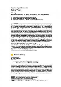
on a graphical model is the main paradigm of iterative decoding. We have also seen that sometimes the iterative decoder fails despite the fact that a unique decoding is possible. Figure 1.44 shows the performance of a so called (3, 6)-regular low-density paritycheck code when transmission takes place over the binary erasure channel under iterative decoding (see Chapter 3). The channel is characterized by the parameter є which denotes the erasure probability of each transmitted bit. This plot is representative of the typical behavior. For increasing lengths the individual curves become PBP B

єBP @ 0.4294

10-1 10-2

0.1

0.2

0.3

0.4

є

i Figure 1.44: ELDPCnx 3 , n x 6 [PBP B (G, є)] as a function of є for n = 2 , i [10]. 2

steeper and steeper and they converge to a limiting asymptotic curve. Of particular importance is the value єBP which marks the zero crossing of this asymptotic curve. For the example given we have єBP @ 0.4294. Its operational meaning is the following: for sufficiently large blocklengths we can achieve arbitrarily small probability of error if we transmit over this channel with channel parameter strictly less than єBP (if the fraction of erased bits is strictly less than єBP ); but if we choose the value of the



25

channel parameter above єBP then the error probability is bounded away from zero. The value єBP acts therefore like a capacity for this particular coding scheme: it separates what is achievable from what is not. The rate of the code is one-half and that єBP @ 0.4294 < 12 = єSha , where єSha denotes the Shannon threshold (the threshold which is achievable with optimal codes and under optimal decoding). This indicates that even in the limit of infinite block lengths we can not achieve capacity with this particular coding scheme. Is this failure to reach capacity due to the code or due to the suboptimal nature of the decoder? We will see that if our example code were decoded optimally the threshold would be єMAP @ 0.48815, which still falls somewhat short of the Shannon threshold one-half. We conclude that both code and decoding algorithm are to blame. Why don’t we just use elements from Shannon’s parity-check ensemble, which we know can achieve capacity? Unfortunately, iterative decoding does not work well on elements of this ensemble. Therefore, in constructing codes that are capable of approaching Shannon capacity under iterative decoding we have to worry about both, constructing good codes (which under optimal decoding could achieve capacity) but also about the performance of the suboptimal decoder compared to the optimal one. Figure 1.44 also gives insight into the finite-length behavior. If we consider each finite-length curve, we see that it can be fairly cleanly separated into two regions – the so called waterfall region in which the error probability falls off sharply and the error floor region in which the curves are much more shallow. We will see that the waterfall region is due to large decoding failures and that in this region the decay of the error probability is exponential in the blocklength. On the other hand, the error floor is due to small failures and in this region the decay is only polynomial. In Figure 1.44 we did not plot the performance of a code but the average performance of an ensemble. It is this ensemble approach which makes an analysis possible. What can we say about the performance of individual instances? For individual instances the contributions stemming from large failures are sharply concentrated around this ensemble average. But the contributions due to small weaknesses in the graph are no longer concentrated. In fact, in the limit of large blocklengths, the distribution of these small weaknesses converges to a well-defined limit. The code design involves therefore two stages. First, we need to find ensembles that exhibit a large threshold (good behavior in the waterfall regime). Within this ensemble we then need to find elements that have few small weaknesses and, therefore, low error floors.


26

introduction

§1.10. Notation, Conventions, and Some Useful Facts Large parts of this book should be accessible to a reader with a standard background in engineering mathematics but no prior background in coding. Some of the less standard techniques that are useful for our investigation are summarized in the appendices. A familiarity with some basic notions of information theory is helpful in places. In fact not much is needed. We sometimes refer to the entropy of a random variable X which we denote by H(X). Entropy is a measure of the “unpredictability” of a random variable. The smaller the entropy the easier it is to predict the outcome of a random experiment. We use small letters for variables and capital letters for random variables. E.g., we say that the random variable X takes on the value x. We write densities as p X (x), and sometimes, if space is an issue, we use the shorthand p(x). In the case that X is discrete with probability distribution p X (x), the entropy is defined as H(X) = − x p X (x) log p X (x). If X has a density then the equivalent quantity is called differential entropy and is defined in the natural way as h(X) = − Ax p X (x) log p X (x)dx. Entropy and differential entropy share the basic properties mentioned below and so we will not make any further notational distinctions and simply refer to entropy. At a few places we invoke the so-called chain rule: if X and Y are random variables then (1.45)

H(X, Y) = H(X) + H(Y X),

where H(Y X) x H(Y X = x)p X (x) and where H(Y X = x) is the entropy of the random variable with probability distribution pY X (y x), where x is fixed. This chain rule is a direct consequence of p X,Y (x, y) = p X (x)pY X (y x) (see Problem 1.23). The rule extends in the natural way to more than two random variables: e.g., H(X, Y , Z) = H(X) + H(Y X) + H(Z X, Y). For the relatively simple channels we are concerned with the Shannon capacity, i.e., the maximal rate at which we can reliably transmit, is given by (1.46)

C = max I(X; Y), p X (x)

where X denotes the input of the channel and Y the output and where the mutual information I(X; Y) is equal to H(X) − H(X Y) = H(Y) − H(Y X). The mutual information I(X; Y) is a measure of how much information Y contains about X (or vice versa). Problem 1.26 re-derives the capacity of the BSC(є) from this general formula. A fundamental fact is that mutual information is non-negative, i.e., I(X; Y) 0 (see Problem 1.24). Using the representation I(X; Y) = H(X) − H(X Y), we see that conditioning does not increase entropy, i.e., (1.47)

H(X) H(X Y).


notation, conventions, and some useful facts

27

We write (1.48)

X,Y ,Z

to indicate that the triple X, Y, and Z forms a Markov chain, i.e., to indicate that p X,Y ,Z (x, y, z) = p X (x)pY X (y x)p Z Y (z y). In this case we have p X,Z Y (x, z y) = p X Y (x y)p Z X,Y (z x, y) = p X Y (x y)p Z Y (z y). In words, if X , Y , Z then X and Z are independent given Y. Conversely, p X,Z Y (x, z y) = p X Y (x y)p Z Y (z y) implies that X , Y , Z. By symmetry of this condition we see that X , Y , Z implies Z , Y , X. We get a Markov chain in a natural way if, for a pair of random variables X and Y, we let Z = f (Y) for some function f (ċ). We make use of the data processing inequality which states that for any triple of random variables X, Y and Z such that X , Y , Z, (1.49)

H(X Y) H(X Z).

Equivalently, I(X; Y) I(X; Z). This is a natural statement: processing can never increase the mutual information. Given a channel pY X (y x) and a function f (ċ), we say that Z f (Y) is a sufficient statistic for X given Y if X , Z , Y, i.e., if X is independent of Y given Z (the relationship X , Y , Z is always true if Z = f (Y) as we have just discussed). A convenient necessary and sufficient condition that Z = f (Y) constitutes a sufficient statistic is that pY X (y x) can be written in the form a(x, z)b(y) for some suitable functions a(ċ, ċ) and b(ċ) (see Problem 1.20). For us the two most important consequences of knowing that Z = f (Y) is a sufficient statistic for X given Y are that (i) the optimum decision on X can be based on Z alone, and that (ii) H(X Y) = H(X Z). The first claim is a direct consequence of the fact that pY X (y x) can be written in the form a(x, z)b(y) and so the second term can be canceled in the MAP rule (see Section 1.5). The second claim follows from the data processing inequality since we know that in this case we have both X , Y , Z (which proves H(X Y) H(X Z)) but also X , Z , Y (which proves H(X Z) H(X Y)). It is helpful to know the Fano inequality: assume we want to estimate the random variable X taking values in the finite alphabet X knowing the (correlated) random variable Y. Let xˆ (y) denote any estimation rule and let Pxˆ (Y) X denote the resulting probability of error. The Fano inequality asserts that (see Problem 1.25) (1.50)

h(P) + P log(X − 1) H(X Y),

where h(x) −x log x − (1 − x) log(1 − x) is the binary entropy function. For the special case where X is a binary random variable the Fano inequality reads (1.51)

h(P) H(X Y).


28

introduction

Random variables X which have a Gaussian distribution appear frequently. In the Gaussian case we have p X (x) = 1 2 exp(−(x − µ)2 (2σ 2 )), where µ is the 2πσ

mean of X, µ = E[X], and σ 2 is the variance of X, σ 2 = E[(X − µ)2 ]. We denote this density by N (µ, σ 2 ). If x is a real parameter taking values in [0, 1], e.g., a probability, we write x¯ for 1 − x. If n N then the set 1, , n is often abbreviated as [n]. Occasionally we want to bound the number of positive roots of a real valued polynomial. Let p(x) di=0 p i x i be a real-valued polynomial of degree d. Consider the associated piecewise linear function whose graph interpolates the points (i, p i ), i 0, . . . , d. We say that p(x) has v sign changes if this associated function crosses the x-axis v times. Example 1.52. Consider the polynomial p(x) = 1 + x 4 − 3.4x 5 + x 11 . The associated piecewise linear graph passes the x-axis twice so that v = 2. Theorem 1.53 (Descarte’s Rules of Signs). Let p(x) be a real-valued polynomial with v sign changes and r positive real roots. Then r v and r − v is even. Example 1.54. Consider again the polynomial p(x) = 1 + x 4 − 3.4x 5 + x 11 . Since v = 2 there exists either no positive root or there are exactly two. In fact, since p(0) = 1 0, p(1) = −0.4 < 0, and p(2) = 1956.2 0 we know that there are exactly two. A numerical calculation shows that the two roots are at x @ 0.89144 and at x @ 1.11519. We frequently need to refer to some basic relations and estimates of factorials and binomials. We summarize them here for reference. (1.55) (1.56) (1.57) (1.58) (1.59) (1.60) (1.61)

n! = B e−s s n ds, '0 n! = 2πn(ne)n (1 + O(1n)), (ne)n n!, k2 n n k k!e− n n k k!, k 1 nh 2 (kn) n 2 , n+1 k m n nh (mn) , m n2, 2 2 k k=0 ' 2n = 4n nπ(1 − 1(8n) + O(n−2 )). n

In general, we make no special distinction between scalars and vectors. In a few places, where confusion might otherwise arise, we denote a vector as x. We assume


notation, conventions, and some useful facts

29

j

that vectors are row vectors. We sometimes write x i as a shorthand for the set of elements x i , x i+1 , , x j . Given a matrix A and a suitable index set I, we let AI denote the submatrix of A, restricted to the columns indexed by I. We use the abbreviations iid to mean independent and identically distributed. If we deal with a set of (random) variables X1 , , Xn it is often convenient to refer to all but one of them. In such a case we write X j as a shorthand for X1 , , X j−1 , X j+1 , , Xn . If f (x) is a convex-D function (we write “convex-D” for a concave function like f (x) = log(x) and “convex-E” for a convex function like x 2 ) and p X (x) is a density then Jensen’s inequality asserts that (1.62)

B f (x)p X (x)dx f $B x p X (x)dx%.

Given a polynomial p(x) (or a function which is analytic around zero) we write coefp(x), x k to denote the coefficient of x k in its Taylor series expansion. E.g., coef(1 + x)n , x k = nk. If n N we say that a function f (n) is O(g(n)) if there exists a constant c so that f (n) cg(n) for all sufficiently large n N. We say that f (n) is o(g(n)) if limn f (n)g(n) = 0. Finally, we write f (n) = Θ(g(n)) if there exist two strictly positive constants c and c so that c g(n) f (n) c g(n) for n sufficiently large. If the underlying parameter n is not clear from context we explicitly denote it by writing On (ċ), on (ċ), and Θ n (ċ). A generic field is denoted by F. The two most important instances for us are the reals, R, as well as the binary field F2 , consisting of 0, 1 with the operations and . If you are not familiar with finite fields, very little is lost if you replace any mention of a generic finite field F with F2 . Unless specifically said otherwise, all performance plots are for ensemble averages and not for specific instances. Expectations are denoted as E[ċ]. This makes the plots reproducible. Of course, typically better performance can be achieved by carefully selecting a specific instance from the ensemble. The end of a definition is marked by , one recognizes the end of an example by the sign , and the user can utter a sigh of relief if she encounters a F while reading a proof. Theorems, lemmas, equations, figures, tables, etc. are labeled by one sequence of consecutive numbers within a chapter. This facilitates locating a referenced item. Maybe slightly unusually, the main text does not contain pointers to the literature. The typical lemma and theorem is a synthesis of either a sequence of papers or has been discovered independently by several authors. Rather than interrupting the flow of ideas in the main text we have opted to collect a history of the developments of the main results at the end of each chapter.


30

introduction

By now, the list of papers in the area of iterative coding measures in the (tens of) thousands. We have therefore not even attempted to give an exhaustive account of references but to give a sufficient number of pointers to the existing literature so that you can locate the relevant material quickly. We apologize to all authors whose papers we have not included in our list. For convenience of the reader we have placed a list of references at the end of each chapter. Each bibliographic entry is followed by a list of numbers within square brackets which indicate the pages on which this particular reference is cited. The order of the exercises roughly follows the order of the topics discussed in the text. We have not ranked the exercises by difficulty. Those exercises that you can solve are easy, the other ones are hard.

Notes Information theory and coding were born in Shannon’s paper “A Mathematical Theory of Communication,” [50]. In was in this paper that Shannon formulated the communications problem as we have presented it in Section 1.2 and where he showed that the transmission task can be broken down into a source coding and a channel coding problem. Our exposition of Shannon’s channel coding theorem for the BSC closely follows van Lint [55]. At around the same time, and working at the same location, Hamming constructed the first class of error-correcting codes, [30]. Interestingly, Hamming’s motivation was not Shannon’s promised capacity but the practical concern of operating a “computing” machine consisting of many relays correctly, despite the fact that every couple of million relay operations an error would occur. A large fraction of the literature on coding for communications was thereafter concerned with finding dense packings of “Hamming”-spheres of radius half the minimum (Hamming) distance. To date there exists an extensive literature on bounds on weight distributions. We refer the reader to the Handbook of Coding Theory [45] which contains several survey articles. The lower bound on the minimum distance which we discuss in Problem 1.11 is due to Gilbert [28]. A similar bound was independently discovered by Varshamov [57]. Asymptotically these two bounds yield the same result, which is the statement discussed in Section 1.4 and in Problem 1.13. The upper bound on the minimum distance stated in Section 1.4 is due to Elias, who presented this result in class lectures in the early sixties. The bound was rediscovered by Bassalygo and first appeared in print in [5]. A substantially tighter upper bound was derived by McEliece, Rodemich, Rumsey, and Welch [42]. It is a tighter version of the linear programming bound based on Delsarte’s association schemes [13]. For a discussion of the weight distribution of random codes (linear and nonlinear) see Barg and Forney


notes

31

[3] and the references therein. The union bound on the performance of a code based on its weight distribution presented in Problem 1.19 is the simplest of a large class of such bounds. A considerably more sophisticated approach was discovered by Gallager in his thesis [24]. A good starting point are the article and the monograph by Sason and Shamai [49, 47] which discuss in depth the relationships between the numerous bounds proposed to date and which contains an exhaustive list of references. In 1971 Cook proved that any problem in NP can be reduced in deterministic polynomial time to the satisfiability problem [11]. Later, Karp showed that, conversely, the satisfiability problem can be reduced to many other problems in NP in deterministic polynomial time and the collection of all these problem is the class of NP-complete problems. The fact that the ML decision problem is NP-complete for binary linear codes was shown by Berlekamp, McEliece and van Tilborg [7] by reducing the problem to three-dimensional matching. The intractability of computing the minimum distance was later shown by Vardy [56]. The classic reference relating to complexity is the book by Garey and Johnson [27]. For survey articles concerning complexity issues in coding theory see Barg [2], Sudan [53], Dumer, Micciancio, and Sudan [15] as well as Spielman [52]. A proof that linear codes achieve capacity on binary-input output-symmetric memoryless channels can be found in Gallager [26]. BCH codes were discovered by Bose and Ray-Chaudhuri [10] and independently by Hocquenghem [33]. Reed-Solomon codes (see Example 1.26), which can be seen as a special case of BCH codes, were proposed around the same time by Reed and Solomon [46]. They have since been rediscovered countless times and are part of many standards and products. Fairly recently, there have been exciting new developments concerning the decoding of Reed-Solomon codes beyond the minimum distance. This development was initiated by Sudan who introduced his list decoding algorithm [54] for Reed-Solomon codes. This was then quickly followed by an improved list decoding algorithm due to Guruswami and Sudan [29]. Further, it was shown by Kötter and Vardy how to turn the list decoding algorithm into a soft-decision decoding algorithm [35]. Convolutional codes (Example 1.32) are due to Elias [16]. The algebraic theory of convolutional codes was developed by Forney in the series of papers [19, 20, 21]. Further excellent references on the theory of convolutional codes are the books by Piret [43], Johannesson and Zigangirov [34], as well as Viterbi and Omura [59], and the survey article by McEliece, which is contained in the collection [45]. Sequential decoding was invented by Wozencraft [62] with important contributions due to Fano [17]. The Viterbi algorithm was originally introduced by Viterbi [58] as a proof technique and it was later pointed out by Forney that it was not only of theoretical interest but also immensely practical. The classical reference is [22].


32

introduction

Forney developed the theory of concatenated codes (see page 20) in his thesis [18]. A simple derivation of the random coding exponent was given by Gallager in [25], extending Shannon’s random coding technique [50]. Further bounds were developed by Shannon, Gallager, and Berlekamp [51]. The equivalent statements for convolutional codes were developed by Yudkin [63], Viterbi [58], and Forney [23]. The currently best known bounds on the error exponent of block codes are due to Barg and McGregor [4]. The principle of iterative decoding was introduced by Gallager in his remarkable thesis for the class of low-density parity-check codes [24] and then revived in a spectacular way by the introduction of turbo codes by Berrou, Glavieux, and Thitimajshima [8]. For a history of the development of iterative coding see the historical notes at the end of Chapters 3 and 4. The representation of Hamming codes via Venn diagrams is due to McEliece [41]. The Descarte’s rule of signs can be found in [14] and [32, Chapter 6]. The idea of performing maximum likelihood decoding of a block code via a trellis, as discussed in Problem 1.17, is due to Bahl, Cocke, Jelinek, and Raviv [1] but the trellis is usually called the Wolf trellis, [61]. The MacWilliams identities, discussed in Problem 1.18, which give a beautiful connection between the weight distribution of a code and its dual, were published by her in [38]. There is a large list of excellent books on classical coding theory. To mention just a few of the most popular ones in alphabetic order: Berlekamp [6], Blahut [9], Lin and Costello [36], MacWilliams and Sloane [39], McEliece [40], Pless [44], and van Lint [55]. A list of survey articles was collected by Pless and Huffman in [45]. For books that focus exclusively on convolutional codes see Johannesson and Zigangirov [34], Piret [43] and Viterbi and Omura [59]. More recently, some books on iterative coding also have become available: Heegard and Wicker [31], Schlegel and Perez [48], and Vucetic and Yuan [60]. Readers interested in information theory need look no further than to Gallager [26] or Cover and Thomas [12]. A further recommended source which spans a wide range of topics is the book by MacKay [37].

Problems 1.1 (Inner Product). Let F be a field and consider the vector space Fn , n N. For u, v Fn define the inner product of u and v by ;u, v> ni=1 u i v i , where all operations are performed in F. Show that this inner product has the following properties 1. ;t + u, v> = ;t, v> + ;u, v>, 2. ;αu, v> = α;u, v>,

t, u, v Fn

α F, u, v Fn


problems

33

3. ;u, v> = ;v, u>, u, v Fn Unfortunately, ;ċ, ċ> is not necessarily an inner product in the mathematical sense: show that for F = F2 , ;u, u> = 0 does not imply u = 0 by exhibiting a counter example. Therefore, F2n , equipped with ;ċ, ċ>, is not an inner-product space. As a consequence, if G is a generator matrix over F2 and H is a corresponding parity-check matrix, then G J K H does not necessarily span the whole space F2n . I.e., the row-space spanned by H is not the orthogonal complement of the row-space spanned by G. Consider, e.g., the generator matrix 1 1 0 0 G=J K 0 0 1 1 and the associated code C(G). Determine C . A code C such that C = C is called self-dual. 1.2 (Extending, Puncturing and Shortening). In this exercise we are concerned with certain simple procedures which allow us to construct new codes from given ones. Assume we have a code C(n, M, d) (not necessarily linear). If d is odd then we can extend the code by appending to each codeword x = (x1 , x n ) the extra symbol x n+1 − ni=1 x i . The inverse operation, namely to delete a symbol, is called puncturing. Finally, consider any subset of codewords which have the same last symbol. Keep only this subset and delete this common symbol. This procedure is called shortening. How do these procedures change the parameters of the code? Under which of these operations do linear codes stay linear? 1.3 (u + v Construction). Assume we are given two binary codes C1 (n, M1 , d1 ) and C2 (n, M2 , d2 ). Define a new code C by C (u, u + v)u C1 , v C2 . Show that C is binary and has parameters C(2n, M1 M2 , d = min(2d1 , d2 )). 1.4 (Proper Codes). Let C be a proper (see Definition 1.21 on page 12) linear code of length n over the field F. Prove that for every position i, 1 i n, and every field element α, α F, the number of codewords that have an α at position i is equal to C F . What happens if the code is not proper? 1.5 (One C, many G). Show that a binary linear code C of length n and dimension k k has 22 Lki=1 2i − 1 distinct k 3 n generator matrices.


34

introduction

1.6 (Conversion of G into Systematic Form). Let G be a k 3 n generator matrix of rank k. Show that G can be brought into systematic form by elementary row/column operations (i.e., permutations of rows/columns, multiplication of a row by a non-zero element of F and addition of one row to another.) Prove that these operations do not change the minimum distance of the code. 1.7 (Conversion G M H). Show that if G is a generator matrix in systematic form, G = (I k P), then H = −P T In−k is a corresponding parity-check matrix. The paritycheck matrix of the [7, 4, 3] binary Hamming code given in (1.25) has the form −P T In−k . Use this fact to write down a corresponding generator matrix G. 1.8 (Singleton Bound). Show that for any code C(n, M, d) over a field F, d n − log F (M) + 1. This is called the Singleton bound. Codes which achieve this bound are called maximum-distance separable (MDS). Hint: Arrange the M codewords of length n in form of a M 3n matrix and delete all but the first Olog F (M)P columns. Argue that the minimum distance between the resulting rows is at most one. 1.9 (Maximum Distance Separable Codes). As discussed in Problem 1.8, a code C which fulfills the Singleton bound is called maximum distance separable (MDS). Examples of such codes are repetition codes with parameters [n, 1, n] and ReedSolomon codes with parameters [n, k, n − k + 1]. Let C be a binary linear code with parameters [n, k] and generator matrix G. Assume that its dual, C , is a MDS code (it has hence parameters [n, n − k, k + 1]). Show that G has the following property. Any subset of [n] of cardinality k is an information set. More precisely, for any such subset and any choice of elements of F at these k positions there is exactly one codeword which agrees with this choice. 1.10 (Hamming Bound). Consider a code C(n, M, d) over a field F. Prove that d−1

M i=02 ni( F − 1)i F n . centered around each codeword. Hint: Consider spheres of radius t d−1 2 Note: A code C which fulfills the Hamming bound with equality is said to be perfect. It is easy to check that binary repetition codes of odd length are perfect codes. Further we saw that all Hamming codes are perfect. Without proof we state that the only other perfect multiple-error correcting codes are the [23, 12, 7] binary Golay code and the [11, 6, 5] ternary Golay code. 1.11 (Gilbert-Varshamov Bound). Show that for any d n, n N, and any field F n F there exist codes C(n, M, d) over F with M d−1 n( F −1)i . i=0

i

Hint: Consider spheres of radius d − 1 centered around each codeword.


problems

35

1.12 (Greedy Code Search Algorithm). The Gilbert-Varshamov bound discussed in Problem 1.11 gives rise to the following greedy code search algorithm. Start by picking a point in Fn where the choice is made with uniform probability. The initial code C consists of this chosen codeword. At any following step in the construction algorithm delete from Fn all codewords currently in C as well as all points contained in spheres of radius (d − 1) around these codewords, where d is the design distance. If the resulting set is non-empty pick another point and add it to C, otherwise the algorithm terminates. Show that this algorithm results in a code C(n, M, d) over F n i with minimum distance at least d and cardinality at least F n d−1 i=0 i ( F − 1) . Note: Such a greedy algorithm does in general not result in a linear code. Surprisingly, the bound is still true, and a slightly modified greedy algorithm still works, if we restrict C to be linear. Define V (F, n, t) ti=0 ni( F − 1)i . Let C0 be the trivial [n, 0, n] code consisting of the zero word only. In general assume that we constructed already the linear [n, k, d] code C k . Such a code contains M = q k codewords. If q k V(F, n, d) q n then we stop and output C. Otherwise proceed as follows. Delete from Fn all codewords of C k as well as all points contained in the spheres of radius (d − 1) around these codewords. Since q k V (F, n, d − 1) < q n , the resulting set is not empty. Pick any element from this set and call it g k+1 . Let C k+1 be the linear code resulting from joining g k+1 to a set of generators g1 , , g k for C k . We claim that C k+1 has minimum distance at least d. Every element c in C k+1 has a representation of the form c = ag k+1 + c where a F and c C k . If a = 0 then w(c ) = w(c) d by assumption that C k is a [n, k, d] code. If on the other hand a 0 then w(c ) = w(ag k+1 + c) = w(g k+1 + a−1 c) = d(g k+1 , −a−1 c) d by our choice of g k+1 and since by linearity −a−1 c C k . 1.13 (Asymptotic Gilbert-Varshamov Bound). Fix F = F2 . Consider codes of increasing blocklength n with 2nr codewords, where r, r (0, 1), is the rate. Let d(C) denote the minimum distance of a code C and define the normalized distance δ = dn. Starting with the Gilbert-Varshamov bound discussed in Problem 1.11, show that δ (r) as define on page 6 fulfills δ (r) h2−1 (1 − r). 1.14 (Pairwise Independence for Generator Ensemble). Let F = F2 and consider the following slight generalization of Shannon’s generator ensemble G(n, k), ˜ k). To sample from G(n, ˜ k) choose a random element C from G(n, k) call it G(n, and a random translation vector c from F2n . The random sample C˜ is C˜ C + c, ˜ k) codewords have a unii.e., a translated version of the code C. Prove that in G(n, form distribution and that pairs of codewords are independent. More precisely, let u[i] i , where i ranges from 0 to 2k − 1, denote the set of binary k-tuples, ordered in some fixed but arbitrary way. For G G(n, k) and c F2n , let x [i] (G, c) c + u[i] G be the i-th codeword. Prove that for j i, PX [j] X [i] = x is uniform, i.e., for any v F2n , PX [j] = v X [i] = x = 21n .


36

introduction

1.15 (Mean and Second Moment for G(n, k)). Consider Shannon’s generator ensemble G(n, k), 0 < k n, as described in Definition 1.27. Recall that its design rate is equal to r = kn. For C G(n, k), let A(C, w) denote the codewords in C of Hamming weight w. Show that 2nr − 1 ¯ A(w = 0), 2n n 2nr − 1 ¯ w 1, EC [A(C, w)] = n A(w), 2 w (2nr − 1)(2nr − 2) n 2 ¯ + , w 1, EC [A2 (C, w)] = A(w) w 22n nr 2 2 −1 n 2 ¯ ¯ EC [(A(C, w) − A(w)) ] = A(w) − 2n , w 1. 2 w EC [A(C, w = 0)] = 1 +

What is the expected number of distinct codewords in an element chosen uniformly at random from G(n, k)? 1.16 (Mean and Second Moment for H(n, k)). Consider Shannon’s parity-check ensemble H(n, k), 0 < k n, as described in Definition 1.27. Recall that its design rate is equal to r = kn. For C H(n, k), let A(C, w) denote the codewords in C of Hamming weight w. Show that A(C, w = 0)] = 1, n ¯ w 1, EC [A(C, w)] = 2−(n−k) A(w), w n n ¯ + − 1 2−2n(1−r) , w 1. EC [A2 (C, w)] = A(w) w w n 2 ¯ ¯ ] = A(w) − 2−2n(1−r) , w 1. EC [(A(C, w) − A(w)) w What is the expected number of distinct codewords in an element chosen uniformly at random from H(n, k)? 1.17 (Wolf Trellis – Bahl, Cocke, Jelinek, and Raviv [1], Wolf [61]). There is an important graphical representation of codes, called trellis. A trellis T = (V , E) of rank n is a finite directed graph with vertex set V and edge set E. Each vertex is assigned a “depth” in the range 0, , n, and each edge connects a vertex at depth i to one at depth i + 1, for some i = 0, 1, , n − 1. The Wolf trellis for a binary linear code C with (n − k) 3 n parity-check matrix H = (h1T , , hnT ), where h Tj is the jth column of H, is defined as follows. At depth i, i = 0, , n, the vertex set consists of 2n−k vertices which we identify with the set of binary (n − k)-tuples. A vertex v at


problems

37

depth i is connected to a vertex u at depth (i + 1) with label λ 0, 1 if there exists a codeword c = (c1 , , cn ) C with c i+1 = λ such that i

i+1

j=1

j=1

v = c j h j and u = c j h j , where by convention 0j=1 c j h j = (0, , 0). Draw the Wolf trellis for the [7, 4, 3] Hamming code with parity-check matrix given in (1.25). There is a one-to-one correspondence between the labeled paths in the Wolf trellis and the codewords of C. Also, many codewords “share” edges and so the total number of edges is, in general, much smaller than the number of codewords times the length of the code. Hence, the Wolf trellis is a compact representation of a code. Many important algorithms can be performed on the trellis of a code (e.g., decoding, determination of minimum distance etc.) We revisit this topic in Section 5.1 when discussing convolutional codes. 1.18 (MacWilliams Identities – MacWilliams [38]). For linear codes there is a simple relationship between the weight distribution of a code and the weight distribution of its dual code. Let C be a binary linear [n, k] code. Let A i , i = 0, , n, be the number of codewords in C of weight i. Note that A0 = 1 and that C = ni=0 A i . We call the collection A i 0in the weight distribution of the code C. The MacWilliams identity states that 1 n Aj = A i Pj (i), 0 j n, C i=0 . where Pj (i) = nl=0 (−1)l li n−i j−l n−i = E=w C(E) for every 0 w n. Here, E denotes 1. Prove that ni=0 A i n−w a subset of 1, , n and E = w denotes a subset of 1, , n of size w. Finally, for a given E, C(E) denotes the subcode of C with zeros outside E. More precisely, C(E) is the collection of those elements of C which have nonzero elements only within the coordinates indexed by E. Note that the zero codeword is always in C(E) so that C(E) is not empty.

2. Let HE denote the submatrix formed by the columns of H that are indexed by E. Prove that C(E) is a binary linear code with dimension dim(C(E)) = w − rank(HE ). 3. Prove that w − rank(HE ) = k − rank(G E¯ ) where E¯ is the complement of E within 1, , n. It can be noticed that this property is also the central element used in Theorem 3.77 (see Lemma 3.75).


38

introduction 4. Let Ai 0in denote the weight distribution of the dual code C . Prove that n−u

(1.63)

i=0

(1.64)

Ai

n−i = C (E) u E=n−u = 2n−u−rank(G E ) E=n−u

(1.65)

= 2n−k−u 2u−rank(H E¯ ) E=n−u u

(1.66)

= 2n−k−u A i i=0

n−i . n−u

j n−i n 1 5. Use i (−1) j−i n− n−i n−w = δ j,w to prove A j = C i=0 A i P j (i), 0 j . Hint: You might have to consider the n, where Pj (i) = nl=0 (−1)l il n−i j−l

generating function ni=0 Pj (i)x i = (1 + x)n−i (1 − x)i and to expand it using 2x n−i ) . the form (1 − x)n (1 + 1−x 6. Use your result to calculate the weight distribution of the dual of the [7, 4, 3] Hamming code. 1.19 (Upper Bound On Error Probability Via Weight Distribution). Consider a linear binary code C of length n and dimension k. Let Aw denote the number of words of weight w and let n

A(D) Aw Dw . w=0

A(D) is called the weight enumerator of the code. Consider the parity-check ensemble H(n, k). Let x be a fixed binary word of length n. Argue that for a randomly chosen element C H(n, k) 1, Px C = −(n−k) , 2

x = 0, otherwise.

Hint: What is the probability that x fulfills one parity-check equation, i.e., that j H i, j x j = 0 for some fixed i? Since H is random Aw is a random variable as well and we denote it by Aw (H). Use the previous result and argue that every code in this ensemble contains the allzero word, in particular A¯0 E[A0 (H)] = 1,


problems

39

and that the expected number of codewords of weight w, w

0, is given by

n A¯w E[Aw (H)] = 2−(n−k) . w Define the average weight enumerator as n

¯ A(D) A¯w Dw . w=0

¯ Using the above result on A¯w and your mastery of formal power sums, write A(D) in a compact form. For a fixed code C, we will now derive a simple upper bound on its block error probability under ML decoding when transmitting over an additive white Gaussian noise channel with noise variance σ 2 . More precisely, assume that the input takes values in 1 and that to each component of the transmitted codeword an iid. Gaussian random variable with variance σ 2 is added. Let Y denote the received word and let xˆML (y) denote the ML decoding rule. Finally, let PB denote the resulting probability of block error. Justify each step in the following sequence PB = PxˆML (Y) 0 X = 0 = PxˆML (Y) C " 0 X = 0 = P max p(Y x) p(Y 0) X = 0 x C0

Pp(Y x) p(Y 0) X = 0

x C0

5 w(x) 8 = Px − Y Y X = 0 = Q σ : x C0 x C0 7 ' n w 1 n w K Aw e− 2σ 2 = Aw Q J σ 2 w=1 w=1 1 1 = QA(e− 2σ 2 ) − A0 R . 2 Collect all the previous results to conclude that the average block error probability for our ensemble can be bounded by 2

2

1 + e− 2σ 2 − 1 1

E[PB (H)]

n

. 2n−k+1 1.20 (Sufficient Statistic). ) Consider transmission of X chosen with probability p X (x) from some code C and let Y denote the received observation. Further, let Z = f (Y), where f (ċ) is a given function. Prove that Z constitutes a sufficient statistic for X given Y if and only if pY X (y x) can be brought into the form a(x, z)b(y) for some suitable functions a(ċ, ċ) and b(ċ).


40

introduction

1.21 (Bound on Binomials). Let 0 k m and k, m N. Justify the following steps. 1 mk

=

k−1 k! k! 2 k! = k e− i=1 ln(1−im) k ek m . m(m − 1) (m − k + 1) m m

1.22 (Bound on Sum of Binomials). Prove the upper bound stated in (1.60). Hint: Consider the binomial identity nk=0 nkx k = (1+x)n with x = m(n−m). 1.23 (Chain Rule). Give a proof of the chain rule H(X, Y) = H(X) + H(Y X). Hint: Write p X,Y (x, y) as p X (x)pY X (y x). 1.24 (Non-Negativity of Mutual Information). Prove that I(X; Y) 0. p (x)p Y (y) and apply the Jensen’s Hint: Write I(X; Y) as − x,y p X,Y (x, y) log Xp X ,Y (x,y) inequality (1.62). 1.25 (Fano Inequality). Prove the Fano inequality (1.50). Hint: Define the random variable E, E 0, 1, which takes on the value 1 if xˆ (Y) X. Expand H(E, X Y) both as H(X Y)+ H(E X, Y) as well as H(E Y)+ H(X E, Y), equate the two terms, and bound H(E X, Y), H(E Y), as well as H(X E, Y). 1.26 (The Capacity of the BSC Rederived). Start with (1.46) to show that the capacity of the BSC(є) is equal to CBSC (є) = 1 − h2 (є).

References [1]

L. Bahl, J. Cocke, F. Jelinek, and J. Raviv, Optimal decoding of linear codes for minimizing symbol error rate, IEEE Trans. Inform. Theory, 20 (1974), pp. 284–287. [32, 36, 40, 61, 63]

[2] A. Barg, Complexity issues in coding theory, in Handbook of Coding Theory, V. S. Pless and W. C. Huffman, eds., Elsevier Science, Amsterdam, 1998, pp. 649–754. [31, 40] [3]

A. Barg and G. D. Forney, Jr., Random codes: Minimum distances and error exponents, IEEE Trans. Inform. Theory, 48 (2002), pp. 2568–2573. [31, 40]

[4] A. Barg and A. McGregor, Distance distribution of binary codes and the error probability of decoding, IEEE Trans. Inform. Theory, 51 (2005), pp. 4237–4246. [32, 40] [5]

L. A. Bassalygo, New upper bounds for error correcting codes, Problemy Peredachi Informatsii, 1 (1965), pp. 41–44. [30, 40]

[6] E. R. Berlekamp, Algebraic Coding Theory, Aegean Park Press, 1984. [32, 40] [7] E. R. Berlekamp, R. J. McEliece, and H. C. A. van Tilborg, On the inherent intractability of certain coding problems, IEEE Trans. Inform. Theory, 24 (1978), pp. 384– 386. [31, 40]


references

41

[8] C. Berrou, A. Glavieux, and P. Thitimajshima, Near Shannon limit error-correcting coding and decoding, in Proceedings of ICC’93, Geneve, Switzerland, May 1993, pp. 1064–1070. [32, 41, 265, 284, 333, 341] [9] R. E. Blahut, Algebraic Codes for Data Transmission, Cambridge University Press, 2003. [32, 41] [10] R. C. Bose and D. K. Ray-Chaudhuri, On a class of error correcting binary group codes, Info. and Control, 3 (1960), pp. 68–79. [31, 41] [11] S. A. Cook, The complexity of theorem proving procedures, in 3rd STOC, 1971, pp. 151– 158. [31, 41] [12] T. M. Cover and J. A. Thomas, Elements of Information Theory, Wiley, New York, 1991. [32, 41] [13] P. Delsarte, An algebraic approach to the association schemes of coding theory. Philips Rsearch Reports Supplements no. 10, 1973. [30, 41] [14] R. Descartes, Geometrie 1636, in A Source Book in Mathematics, Harvard Univ. Press, Cambridge, 1969. [32, 41] [15] I. Dumer, D. Micciancio, and M. Sudan, Hardness of approximating the minimum distance of a linear code, IEEE Trans. Inform. Theory, 49 (2003), pp. 22–37. [31, 41] [16] P. Elias, Coding for noisy channels, in IRE International Convention Record, Mar. 1955, pp. 37–46. [31, 41] [17] R. M. Fano, A heuristic discussion of probabilistic decoding, IEEE Trans. Inform. Theory, 9 (1963), pp. 64–74. [31, 41] [18] G. D. Forney, Jr., Concatenated Codes, PhD thesis, MIT, 1966. [32, 41] [19]

, Convolutional codes I: Algebraic structure, IEEE Trans. Inform. Theory, 16 (1970), pp. 720–738. [31, 41, 332, 342]

[20]

, Correction to ‘convolutional codes I: Algebraic structure’, IEEE Trans. Inform. Theory, 17 (1971), p. 360. [31, 41, 332, 342]

[21]

, Structural analysis of convolutional codes via dual codes, IEEE Trans. Inform. Theory, 19 (1973), pp. 512–518. [31, 41]

[22]

, The Viterbi algorithm, IEEE Proceedings, 61 (1973), pp. 268–278. [31, 41]

[23]

, Convolutional codes II: Maximum-likelihood decoding, Inform. Contr., 25 (1974), pp. 222–266. [32, 41, 332, 342]

[24] R. G. Gallager, Low-density parity-check codes, IRE Transactions on Information Theory, 8 (1962), pp. 21–28. [31, 32, 41, 61, 64, 155, 165, 267, 285, 417, 421, 431, 432] [25]

, A simple derivation of the coding theorem and some applications, IEEE Trans. Inform. Theory, 11 (1965), pp. 3–18. [32, 41]


42 [26]

introduction , Information theory and reliable communication, Wiley, 1968. [31, 32, 42]

[27] M. R. Garey and D. S. Johnson, Computers and Intractability: A Guide to the Theory of NP-Completeness, W. H. Freeman, 1979. [31, 42] [28] E. N. Gilbert, A comparison of signaling alphabets, Bell System Tech. J., 31 (1952), pp. 504–522. [30, 42] [29] V. Guruswami and M. Sudan, Improved decoding of Reed-Solomon and algebraicgeometry codes, in Proceedings 39th Symp. Foundations Comput Sc., 1998. [31, 42] [30] R. W. Hamming, Error detecting and error correcting codes, Bell System Tech. J., 26 (1950), pp. 147–160. [30, 42] [31] C. Heegard and S. B. Wicker, Turbo Coding, Kluwer Academic Publ., 1999. [32, 42, 61, 64] [32] P. Henrici, Applied and Computational Complex Analysis, Vol. 1, John Wiley & Sons, New York, 1974. [32, 42] [33] A. Hocquenghem, Codes correcteurs d’erreurs, Chiffres, 2 (1959), pp. 147–156. [31, 42] [34] R. Johannesson and K. S. Zigangirov, Fundamentals of Convolutional Coding, IEEE Press, 1999. [31, 32, 42, 332, 343] [35] R. Kötter and A. Vardy, Algebraic soft-decision decoding of Reed-Solomon codes, IEEE Trans. Inform. Theory, 49 (2003), pp. 2809–2825. [31, 42] [36] S. Lin and D. J. Costello, Jr., Error Control Coding, Prentice-Hall, 2nd ed., 2004. [32, 42] [37] D. J. C. MacKay, Information Theory, Inference, and Learning Algorithms, Cambridge University Press, 2003. [32, 42] [38] F. J. MacWilliams, A theorem on the distribution of weights in a systematic code, Bell System Tech. J., 42 (1963), pp. 79–94. [32, 37, 42] [39] F. J. MacWilliams and N. J. Sloane, The Theory of Error-Correcting Codes, NorthHolland, 1977. [32, 42] [40] R. J. McEliece, The theory of information and coding : a mathematical framework for communication, Addison-Wesley, 1977. [32, 42] [41]

, The 2004 Shannon lecture, in Proc. of the IEEE Int. Symposium on Inform. Theory, Chicago, USA, June 27 – July 2 2004, IEEE. [32, 42]

[42] R. J. McEliece, E. R. Rodemich, H. Rumsey, Jr., and L. R. Welch, New upper bounds on the rate of a code via the Delsarte-MacWilliams inequalities, IEEE Trans. Inform. Theory, 23 (1977), pp. 157–166. [30, 42] [43] P. M. Piret, Convolutional Codes: An Algebraic Approach, MIT Press, 1988. [31, 32, 42, 332, 344]


references

43

[44] V. S. Pless, Introduction to the Theory of Error-Correcting Codes, John Wiley and Sons, 1989. [32, 43] [45] V. S. Pless and W. C. Huffman, eds., Handbook of Coding Theory, Elsevier Science, Amsterdam, 1998. [30–32, 43] [46] I. S. Reed and G. Solomon, Polynomial codes over certain finite fields, J. SIAM, 8 (1960), pp. 300–304. [31, 43] [47] I. Sason and S. Shamai, Performance Analysis of Linear Codes under MaximumLikelihood Decoding: A Tutorial, vol. 3 of Foundations and Trends in Communications and Information Theory, NOW, Delft, the Netherlands, July 2006. [31, 43] [48] C. Schlegel and L. C. Perez, Trellis and Turbo Coding, Wiley-IEEE Press, 2004. [32, 43] [49] S. Shamai and I. Sason, Variations on the Gallager bounds, connections, and applications, IEEE Trans. Inform. Theory, 48 (2002), pp. 3029–3051. [31, 43] [50] C. E. Shannon, A mathematical theory of communication, Bell System Tech. J., 27 (1948), pp. 379–423, 623–656. [30, 32, 43] [51] C. E. Shannon, R. G. Gallager, and E. R. Berlekamp, Lower bounds to error probability for coding on discrete memoryless channels - II, Inform. Contr., 10 (1967), pp. 522– 552. [32, 43] [52] D. A. Spielman, The complexity of error-correcting codes, Lectures Notes in Computer Science, 1279 (1997), pp. 67–84. [31, 43] [53] M. Sudan, Algorithmic issues in coding theory, in 17-th Conference on Foundations of Software Technology and Theoretical Computer Science, Kharagpur, India, 1997. [31, 43] [54]

, Decoding Reed-Solomon codes beyond the error-correction diameter, in Proc. 35th Annual Allerton Conference on Communication, Control and Computing, Monticello, IL, 1997. [31, 43]

[55] J. H. van Lint, Introduction to coding theory, Springer Verlag, second ed., 1992. [30, 32, 43] [56] A. Vardy, The intractability of computing the minimum distance of a code, IEEE Trans. Inform. Theory, 43 (1997), pp. 1757–1766. [31, 43] [57] R. R. Varshamov, Estimate of the number of signals in error correcting codes, Doklady Akad. Nauk SSSR, 117 (1957), pp. 739–741. [30, 43] [58] A. J. Viterbi, Error bounds of convolutional codes and an asymptotically optimum decoding algorithm, IEEE Trans. Inform. Theory, 13 (1967), pp. 260–269. [31, 32, 43, 61, 65]


44

introduction

[59] A. J. Viterbi and J. K. Omura, Principles of Digital Communication and Coding, McGraw-Hill, 1979. [31, 32, 44] [60] B. Vucetic and J. Yuan, Turbo codes: principles and applications, Kluwer Academic Publ., 2000. [32, 44] [61] J. K. Wolf, Efficient maximum likelihood decoding of linear block codes using a trellis, IEEE Trans. Inform. Theory, 24 (1978), pp. 76–80. [32, 36, 44] [62] J. M. Wozencraft, Sequential decoding for reliable communication, Research Lab. of Electronis Tech. Rept. 325, MIT, Cambridge, MA, 1957. [31, 44] [63] H. L. Yudkin, Channel state testing in information decoding, PhD thesis, MIT, Cambridge, MA, 1964. [32, 44]


Chapter 2

FAC T O R G R A P H S We start with a general task: how can we efficiently compute marginals of multivariate functions. A large class of problems can be phrased in this way. The decoding problem, which is the focus of this book, is one important such instance.

§2.1. Distributive Law Let F be a field (think of F = R) and let a, b, c F. The distributive law states that ab + ac = a(b + c).

(2.1)

This simple law, properly applied, can lead to significant reductions in computational complexity: consider e.g. the evaluation of i, j a i b j as (i a i )( j b j ). The factor graph approach represents the appropriate framework to systematically take advantage of instances where the distributive law can be applied. We start with an example. Consider a function f with factorization (2.2)

f (x1 , x2 , x3 , x4 , x5 , x6 ) = f1 (x1 , x2 , x3 ) f2 (x1 , x4 , x6 ) f3 (x4 ) f4 (x4 , x5 ).

We are interested in the marginal of f with respect to x1 . By some abuse of notation, we denote this marginal by f (x1 ), f (x1 )

x 2 ,x 3 ,x 4 ,x 5 ,x 6

f (x1 , x2 , x3 , x4 , x5 , x6 ) = f (x1 , x2 , x3 , x4 , x5 , x6 ). x 1

In the previous line we introduced the notation ... to denote a summation over all variables contained in the expression except the ones listed. This convention will save us from a flood of subscripts. Assume that all variables take values in a finite alphabet, call it X . Determining f (x1 ) for all values of x1 by brute force requires Θ X 6 operations, where we assume a somewhat naive computational model in which all operations (addition, multiplication, function evaluations, ...) have constant cost. But we can do better: taking advantage of the factorization, we can rewrite f (x1 ) as f (x1 ) = Q f1 (x1 , x2 , x3 )RQ f2 (x1 , x4 , x6 ) f3 (x4 ) f4 (x4 , x5 )R. x 2 ,x 3

x 4 ,x 6

x5

Fix x1 . The evaluation of the first factor can be accomplished with Θ X 2 operations. The second factor depends only on x4 , x5 and x6 . It can be evaluated efficiently in the following manner. For each value of x4 , determine x5 f4 (x4 , x5 ) and store 45 Preliminary version – January 24, 2007

46

factor graphs

the result. This has computational complexity Θ X 2 and requires Θ (X ) storage. Now multiply by f2 (x1 , x4 , x6 ) f3 (x4 ) and sum over x4 and x6 . Therefore, the evaluation of the second factor requires Θ X 2 operations as well. Since there are X values for x1 , the overall task has complexity Θ X 3 . This compares favorably to Θ X 6 , the complexity of the brute force approach.

§2.2. Graphical Representation of Factorizations Consider a function and its factorization. (As an example we will use the function and factorization given in (2.2).) Associate with this factorization a factor graph as follows. For each variable draw a variable node (circle) and for each factor draw a factor node (square). Connect a variable node to a factor node by an edge if and only if the corresponding variable appears in this factor. The resulting graph for our running example is shown on the left of Figure 2.3. The factor graph is bipartite. This means that the set of vertices is partitioned into two groups (the set of nodes corresponding to variables and the set of nodes corresponding to factors) and that an edge always connects a variable node to a factor node. For our particular example the factor graph is a (bipartite) tree. This means that there are no cycles in the graph, i.e., there is one and only one path between each pair of nodes. As we will show x1 f2

f1 x2

x3

x4 f3

x6 f4

x7 x6 x5 x4 x3 x2 x1

½x 4 +x 5 +x 7 =0 ½x 3 +x 4 +x 6 =0 ½x 1 +x 2 +x 4 =0

x5

Figure 2.3: Left: Factor graph of f given in (2.2). Right: Factor graph for the code membership function defined in Example 2.4. in the next section, in this important special case there is a simple message-passing algorithm for computing marginals efficiently. Everything that follows remains true in the slightly more general scenario where the factor graph forms a forest, i.e., the factor graph is disconnected and it is composed of a collection of trees. In order to keep things simple our language will reflect the case of a single tree and we ignore this straightforward generalization.


recursive determination of marginals

47

Example 2.4 (Special Case: Tanner Graph). Consider the binary linear code C(H) defined by the parity-check matrix x1 1 H= 5 60 70

x2 1 0 0

x3 0 1 0

x4 1 1 1

x5 0 0 1

x6 0 1 0

x7 08 . 09 1:

Let F2 denote the binary field with elements 0, 1. The function f (x1 , , x7 ), taking inputs in F72 , 1, if Hx T = 0T , f (x1 , , x7 ) 0, otherwise, where x = (x1 , , x7 ), tests membership in C(H). We can factor f as f (x1 , . . . , x7 ) = ½x1 +x2 +x4 =0 ½x3 +x4 +x6 =0 ½x4 +x5 +x7 =0 . The symbol ½ċ denotes an indicator function which is 1 if the condition inside the braces is fulfilled and 0 otherwise. The corresponding factor graph is shown on the right in Figure 2.3. The factor graph for the function f , deciding code membership in the code C(H), is called the Tanner graph of H. We will have much more to say about it in Section 3.3.

§2.3. Recursive Determination of Marginals Consider the factorization of a generic function g and assume that the associated factor graph is a tree (by definition it is always bipartite). Assume we are interested in the marginalization of g with respect to the variable z, i.e., we are interested in g(z) z g(z, . . . ). Since by assumption the factor graph of g is a bipartite tree, g has a generic factorization of the form K

g(z, . . . ) = S [g k (z, . . . )] k=1

for some integer K with the following crucial property: z appears in each of the factors g k , but all other variables appear in only one factor. For our running example this is the factorization f (x1 , . . . ) = [ f1 (x1 , x2 , x3 )] [ f2 (x1 , x4 , x6 ) f3 (x4 ) f4 (x4 , x5 )] , so that K = 2. The generic factorization and the particular instance for our running example f are shown in Figure 2.5. Taking into account that the individual factors


48

factor graphs g

x1

z

f

f1

[g1 ] [g k ] [g K ]

f2 x2 x3

x4

[ f1 ]

f3

x6 f4 x5

[ f2 f3 f4]

Figure 2.5: Generic factorization and the particular instance.

g k (z, . . . ) only share the variable z, an application of the distributive law leads to K

(2.6)

K

g(z, . . . ) = S [g k (z, . . . )] = SQ g k (z, . . . )R . z

z k=1

k=1 z

TUU U U U U U U U U U U U U U U U U U U U U U UV U U U U U U U U U U U U U U U U U U U U U U U W

TUU U U U U U U U U U U U U U U U U U U U U U VU U U U U U U U U U U U U U U U U U U U U U U W

marginal of product

product of marginals

In words, the desired marginal z g(z, . . . ) is the product of the individual marginals z g k (z, . . . ). In terms of our running example we have f (x1 ) = Q f1 (x1 , x2 , x3 )RQ f2 (x1 , x4 , x6 ) f3 (x4 ) f4 (x4 , x5 )R. x 1

x 1

This single application of the distributive law leads, in general, to a non-negligible reduction in complexity. But we can go further and apply the same idea recursively to each of the terms g k (z, . . . ). Note that each g k is itself a product of factors. In Figure 2.5 these are the factors of g which are grouped together in one of the ellipsoids. Since the factor graph is a bipartite tree, g k must in turn have a generic factorization of the form J

g k (z, . . . ) = h(z, z1 , . . . , z J ) S 1h j (z j , . . . )2, TUU U U U U U U U U U U U U U U U U VU U U U U U U U U U U U U U U U U U W j=1 TUU U U U U U U U U U U U UV U U U U U U U U U U U U U W kernel

factors

where z appears only in the “kernel” h(z, z1 , . . . , z J ) and each of the variables z j appears at most twice, possibly in the kernel and possibly in one of the factors h j(z j , . . . ). All other variables are again unique to a single factor. For our running example we


recursive determination of marginals

49

have for [ f2 f3 f4 ] f2 (x1 , x4 , x6 ) f3 (x4 ) f4 (x4 , x5 ) = f2 (x1 , x4 , x6 ) [ f3 (x4 ) f4 (x4 , x5 )] [1] . TUU U U U U U U U U U U U U UV U U U U U U U U U U U U U U W TUU U U U U U U U U U U U U U U U U U U U U U U V U U U U U U U U U U U U U U U U U U U U U U U UW Z x6

x4

kernel

The generic factorization and the particular instance for our running example f are shown in Figure 2.7. Another application of the distributive law leads to x1

z kernel z1

kernel

h

zj

zJ

f2

x4

[h 1 ] [h j ] [h J ]

x6

f3

f4

[1]

x5 [ f3 f4 ] [ f2 f3 f4]

[g k ]

Figure 2.7: Generic factorization of g k and the particular instance.

J

g k (z, . . . ) = h(z, z1 , . . . , z J ) S 1h j (z j , . . . )2 z

z

j=1 J

(2.8)

= h(z, z1 , . . . , z J ) SQ h j (z j , . . . )R . z

j=1 z j

TUU U U U U U U U U U U U U U U U U U U U U U U VUU U U U U U U U U U U U U U U U U U U U U U U U W product of marginals

In words, the desired marginal z g k (z, . . . ) can be computed by multiplying the kernel h(z, z1 , . . . , z J ) with the individual marginals z j h j (z j , . . . ) and summing out all remaining variables other than z. We are back to where we started. Each factor h j (z j , . . . ) has the same generic form as the original function g(z, . . . ), so that we can continue to break down the marginalization task into smaller pieces. This recursive process continues until we have reached the leaves of the tree. At the leaf nodes the task is simple. A function leaf node has the generic form g k (z), so that z g k (z) = g k (z): this means that the initial message sent by a function leaf node is the function itself. To find out the


50

factor graphs

correct initialization at a variable leaf node consider the simple example of computing f (x1 ) = x1 f (x1 , x2 ). Here, x2 is the variable leaf node. By the messagepassing rule (2.8) the marginal f (x1 ) is equal to x1 f (x1 , x2 )ċ µ(x2 ), where µ(x2 ) is the initial message that we send from the leaf variable node x2 towards the kernel f (x1 , x2 ). We see that in order to get the correct result this initial message should be the constant message 1.

§2.4. Efficient Marginalization Via Message Passing In the previous section we have seen that, in the case where the factor graph is a tree, the marginalization problem can be broken down into smaller and smaller tasks according to the structure of the tree. This gives rise to the following efficient message-passing algorithm. The algorithm proceeds by sending messages along the edges of the tree. Messages are functions on X , or, equivalently, vectors of length X . The messages signify marginals of parts of the function and these parts are combined to form the marginal of the whole function. Message-passing originates at the leaf nodes. Messages are passed up the tree and as soon as a node has received messages from all its children, the incoming messages are processed and the result is passed up to the parent node. Example 2.9 (Message-Passing Algorithm for the Running Example). Consider this procedure in detail for the case of our running example as shown in Figure 2.10. The top left-most figure shows the factor graph. Message-passing starts at the leaf nodes as shown in the middle figure on the top. The variable leaf nodes x2 , x3 , x5 and x6 send the constant function 1 as discussed at the end of the previous section. The factor leaf node f3 sends the function f3 up to its parent node. In the next time step the factor node f1 has received messages from both its children and can therefore proceed. According to (2.8), the message it sends up to its parent node x1 is the product of the incoming messages times the “kernel” f1 , after summing out all variable nodes except x1 , i.e., the message is x1 f1 (x1 , x2 , x3 ). In the same manner factor node f4 forwards to its parent node x4 the message x4 f4 (x4 , x5 ). This is shown in the right-most figure in the top row. Now variable node x4 has received messages from all its children. It forwards to its parent node f2 the product of its incoming messages, in agreement with (2.6), which says that the marginal of a product is the product of the marginals. This message, which is a function of x4 , is f3 (x4 ) x4 f (x4 , x5 ) = x4 f3 (x4 ) f4 (x4 , x5 ). Next, function node f2 can forward its message, and, finally, the marginalization is achieved by multiplying all incoming messages at the root node x1 . Before stating the message-passing rules formally, there is one important observation which we must stress. So far we have considered the marginalization of a


efficient marginalization via message passing x1

x1 f2

f1 x2

x3

x4

x6 f3

f4

1 x2

f1 1 x3 x4 f3

x5

x1

f2

x6 f3 x5

x 1 f 1 f2 f1 1 1 1 x2 x3 x4 x6 x 4 f 4 f3 f3 f4 x 4 f 3 f 4 1 x5

x1

x 1 f 1 f1 1 1 x2 x3 x4 f3 x 4 f 3 f 4

1

f4 1

x1 x 1 f 1 f1 1 1 x2 x3 x4 f3

51

f2

1 x6 x 4 f 4 f3 f4 1 x5

x 1 f 1 f 2 f 3 f 4 x1 x 1 f 2 f 3 f 4 x 1 f 1 x 1 f 2 f 3 f 4 f2 f2 f1 1 1 1 1 x2 x3 x4 x6 x6 x 4 f 4 x 4 f 4 f3 f3 f4 f3 f4 x 4 f 3 f 4 1 1 x5 x5

Figure 2.10: Marginalization of function f via message passing. Message passing starts at the leaf nodes. A node which has received messages from all its children processes the messages and forwards the result to its parent node. Bold edges indicate edges along which messages have already been sent.

function f with respect to a single variable x1. We have seen that this marginalization can be performed efficiently if the factor graph of f is a tree, where the complexity of the computation essentially depends on the largest degree of the factor graph and the size of the underlying alphabet. Assume now we are interested in computing all marginals. We can draw for each variable a tree rooted in this variable and execute the message-passing algorithm on each rooted tree. But it is easy to see that the algorithm does not depend on the root of the tree and that in fact all the computations can be performed simultaneously on a single tree. Simply start at all leaf nodes and for every edge compute the outgoing message along this edge as soon as you have received the incoming messages along all other edges which connect to the given node. Continue in this fashion until a message has been sent along both directions of every edge. Computing all marginals is therefore only slightly more complex than computing a single marginal. We now summarize the set of message-passing rules. Messages, which we denote by µ, are functions on X . Message passing starts at leaf nodes. Consider a node and one of its adjacent edges, call it e. As soon as the incoming messages to the node along all other adjacent edges have been received these messages are processed and the result is sent out along e. This process continues until messages along all edges in the tree have been processed. In the final


52

factor graphs

step the marginals are computed by combining all messages which enter a particular variable node. The initial conditions and processing rules are summarized in Figure 2.11. Since the messages represent probabilities or beliefs the algorithm is also known as the belief propagation (BP) algorithm. From now on we will mostly refer to it under this name. x f µ(x) = L Kk=1 µ k (x) f

µ1 f1

µ(x) = 1 x

µ(x) = x f (x, x 1 , , x J ) L Jj=1 µ j (x j ) x

variable/function node processing

x µk µK fk

f

initialization at leaf nodes

µ(x) = f (x)

f µj

µ1 x1

fK f K+1

marginalization µ1 f1

xj

µJ

xJ

µ K+1 x LK+1 k=1 µ k (x) µk µK fK

fk

Figure 2.11: Message-passing rules. The top row shows the initialization of the messages at the leaf nodes. The middle row corresponds to the processing rules at the variable and function nodes, respectively. The bottom row explains the final marginalization step.

§2.5. Decoding via Message Passing §2.5.1. Bitwise MAP Decoding Assume we transmit over a binary-input (X i 1) memoryless (pY X (y x) = Lni=1 pYi X i (y i x i )) channel using a linear code C(H) defined by its parity-check matrix H and assume that codewords are chosen uniformly at random. The rule for the bitwise MAP decoder reads: xîMAP (y) = argmaxx i 1 p X i Y (x i y) (law of total probability)

= argmaxx i 1 p X Y (x y) x i


decoding via message passing (Bayes)

= argmaxx i 1 pY X (y x)p X (x)

(2.12)

= argmaxx i 1 JS pY j X j (y j x j )K½x C ,

53

x i

x i

j

where in the last step we have used the fact that the channel is memoryless and that codewords have uniform prior. In the above formulation we consider y as a constant (since it is to the decoding algorithm as an input). Therefore, we write x i to indicate a summation over all components of x except x i . Assume that the code membership function ½x C has a factorized form. From (2.12) it is then clear that the bitwise decoding problem is equivalent to calculating the marginal of a factorized function and choosing the value which maximizes this marginal. Example 2.13 (Bitwise MAP Decoding). Consider the parity-check matrix given in Example 2.4. In this case argmaxx i 1 p X i Y (x i y) can be factorized as 7

argmaxx i 1 JS pYi X j (y j x j )K½x1 +x2 +x4 =0 ½x3 +x4 +x6 =0 ½x4 +x5 +x7 =0 . x i

j=1

The corresponding factor graph is shown in Figure. 2.14. This graph includes the p(y7 x 7 ) p(y6 x 6 ) p(y5 x 5 ) p(y4 x 4 ) p(y3 x 3 ) p(y2 x 2 ) p(y1 x 1 )

½x 4 +x 5 +x 7 =0 ½x 3 +x 4 +x 6 =0 ½x 1 +x 2 +x 4 =0

Figure 2.14: The factor graph for the MAP decoding of our running example. Tanner graph of H, but in addition also contains the factor nodes which represent the effect of the channel. For this particular case the resulting graph is a tree. We can therefore apply the message-passing algorithm to this example in order to perform bit MAP decoding. §2.5.2. Simplification of Message-Passing Rules for Bitwise MAP Decoding In the binary case a message µ(x) can be thought of as a real-valued vector of length two, (µ(1), µ(−1)) (here we think of the bit values as 1). The initial such message emitted by variable leaf node i is (pYi X i (y i 1), pYi X i (y i − 1)) (see Figure 2.14). Recall that at a variable node of degree (K + 1) the message-passing rule


54

factor graphs

calls for a pointwise multiplication, K

K

µ(1) = S µ k (1),

µ(−1) = S µ k (−1).

k=1

k=1

Introduce the ratio r k µ k (1)µ k (−1). The initial such ratios are the likelihood ratios associated with the channel observations. We have r=

K µ(1) LK µ k (1) = Kk=1 = S rk , µ(−1) Lk=1 µ k (−1) k=1

i.e., the ratio of the outgoing message at a variable node is the product of the incoming ratios. If we define the log-likelihood ratios l i = ln(r i ), then the processing rule reads l = Kk=1 l i . Consider now the ratio of an outgoing message at a check node which has degree (J + 1). For a check node the associated “kernel” is f (x, x1 , . . . , x J ) = ½ J

j=1

x j =x .

Since in the current context we assume that the x i take values in 1 (and not F2 ) we wrote L Jj=1 x j = x (instead of Jj=1 x j = x). We therefore have J x f (1, x1 , . . . , x J ) L j=1 µ j (x j ) µ(1) = r= µ(−1) x f (−1, x1 , . . . , x J ) L Jj=1 µ j (x j )

=

(2.15)

=

J x j =1 L j=1

µ j (x j )

J L j=1 j=1 x j =−1

µ j (x j )

x1 ,...,x J J

j=1

x1 ,...x J J

x1 ,...,x J J

j=1

x1 ,...,x J J

j=1

=

j=1

x1 ,...,x J J

j=1

(1+x j )2 J x j =1 L j=1 r j J

x1 ,...,x J J

(1+x j )2

x j =−1 L j=1 r j

=

µ j (x j ) J x j =1 L j=1 µ j (−1)

µ j (x j ) J x j =−1 L j=1 µ j (−1)

J

J

J

J

L j=1 (r j + 1) + L j=1 (r j − 1) L j=1 (r j + 1) − L j=1 (r j − 1)

.

The last step warrants some remarks. If we expand out L Jj=1 (r j + 1), then we get the sum of all products of the individual terms r j , j = 1, , J. E.g., L3j=1 (r j + 1) = 1 + r1 + r2 + r3 + r1 r2 + r1 r3 + r2 r3 + r1 r2 r3 . Similarly, LJj=1 (r j − 1) is the sum of all products of the individual terms r j , where all products consisting of d terms such that J − d is odd have a negative sign. E.g., we have L3j=1 (r j − 1) = −1 + r1 + r2 + r3 − r1 r2 − r1 r3 − r2 r3 + r1 r2 r3 . From this follows that J

J

j=1

j=1

S(r j + 1) + S(r j − 1) = 2

x 1 ,...,x J Jj=1


J

(1+x j )2

S rj

x j =1 j=1

.

decoding via message passing

55

Applying the analogous reasoning to the denominator, the equality follows. If we divide both numerator and denominator by LJj=1 (r j + 1), we see that (2.15) is equivalent to the statement r =

1+ j 1− j

r j −1 r j +1 r j −1

, which in turn implies

r j +1

r−1 r+1 = tanh(l2). Combining theses r j −1 J J L j=1 r j +1 = L j=1 tanh(l j 2), so that

r = el we see that tanh(l2) =

r−1 r+1

=

r−1 r+1

= Lj

r j −1 r j +1 .

From

two statements we have

J

l = 2 tanh−1 JS tanh(l j 2)K.

(2.16)

j=1

We summarize: in the case of transmission over a binary channel the messages can be compressed to a single real quantity. In particular, if we choose this quantity to be the log-likelihood ratio (log of the ratio of the two likelihoods) then the processing rules take on a particularly simple form: at variables nodes messages add, and at check nodes the processing rule is stated in (2.16). §2.5.3. Forney-Style Factor Graphs Factor graphs (FG) represent one particular language to formulate the relationship between a function and its local components. One popular alternative is the representation in terms of Forney-style factor graphs (FSFG). x1 x2 x3 x4

x2 x3 x4

x1

Figure 2.17: Left: A standard FG in which each variable node has degree at most two. Right: The equivalent FSFG. The variables in the FSFG are associated with the edges in the FG. Consider the FG shown in the left hand side of Figure 2.17. Note that each variable node has degree one or two. We can therefore convert the bipartite graph into a regular (in the sense of not bipartite) graph by representing variable nodes as (half)edges. The result is shown on the right hand side of Figure 2.17. This is the FSFG representation. In general, a variable node might have degree larger than two. In this case it is easy to replicate such a variable node a sufficient number of times by an equality factor as shown in Figure 2.18. The left side shows a variable node of degree K + 1. The right side shows the representation as a FSFG. The K additional variables x1 , , x K are enforced to be equal to the original variable x by an “equality factor”, i.e., x = x1 = = x K . Figure 2.19 compares the standard FG for the MAP


56

factor graphs

x xK

=

x k x K−1

x1

Figure 2.18: Representation of a variable node of degree K as a FG (left) and the equivalent representation as a FSFG (right).

decoding problem of our running example with the corresponding FSFG. p(y7 x 7 ) p(y6 x 6 ) p(y5 x 5 ) p(y4 x 4 ) p(y3 x 3 ) p(y2 x 2 ) p(y1 x 1 )

½x 4 +x 5 +x 7 =0 ½x 3 +x 4 +x 6 =0 ½x 1 +x 2 +x 4 =0

p(y7 x 7 ) p(y6 x 6 ) p(y5 x 5 ) p(y4 x 4 ) p(y3 x 3 ) p(y2 x 2 ) p(y1 x 1 )

½x 4 +x 5 +x 7 =0 =

½x 3 +x 4 +x 6 =0 ½x 1 +x 2 +x 4 =0

Figure 2.19: The standard FG and the corresponding FSFG for the MAP decoding problem of our running example. The relationship between the standard FG and the FSFG is straightforward and little effort is required to move from one representation to the other. The messagepassing rules carry over verbatim. In fact, in the setting of FSFGs we only need the factor node processing rule: for a generic node of degree (J + 1), the outgoing message along edge x is J

(2.20)

µ(x) = f (x, x1 , , x J ) S µ j (x j ). x

j=1

Recall that variables in the FSFG are represented by edges. Some thought shows that in order to compute the final marginalization with respect to a certain variable, we need to multiply the two messages that flow along the corresponding edge. FSFGs have fewer nodes and are therefore typically simpler. As a drawback, we sometimes end up with “half-edges” as in Figure 2.17. §2.5.4. Generalization to Commutative Semirings We started with a discussion of the distributive law assuming that the underlying algebraic structure was a field F and used it to derive efficient marginalization algorithms. A closer look at our derivation shows that actually all that was needed was the fact that we were working in a commutative semiring. In a commutative semiring K the two operations, which we call “+” and “ċ” satisfy the following axioms: (i) the


decoding via message passing K “(+, 0)” “(ċ, 1)” F (+, 0) (ċ, 1) F[x, y, ] (+, 0) (ċ, 1) (+, 0) (ċ, 1) R0 (ċ, 1) R0 E\ (min, \) (max, 0) (ċ, 1) R0 R E\ (min, \) (+, 0) R E−\ (max, −\) (+, 0) ( , 1) 0, 1 (, 0)

57

description

sum-product min-product max-product min-sum max-sum Boolean

Table 2.21: A list of commutative semirings which are relevant for iterative coding. The entry F[x, y, ] denotes the set of polynomials in the variables x, y, . . ., with coefficients in the field F, and the usual polynomial arithmetic. operations “+” and “ċ” are commutative (x + y = y + x; x ċ y = y ċ x) and associative (x + (y + z) = (x + y) + z; x ċ (y ċ z) = (x ċ y) ċ z) with identity elements denoted by “0” and “1”, respectively; (ii) the distributive law (x + y) ċ z = (x ċ z) + (y ċ z) holds for any triple x, y, z K. In comparison to a field F we do not require the existence of an inverse with respect to either operation. Table 2.21 lists several commutative semirings which are useful in the context of coding. The task of verifying that each of these examples indeed fulfills the stated axioms is relegated to Problem 2.1. The most important example in the context of iterative coding is the so-called sum-product semiring, in which the two operations are standard addition and multiplication (this is the example which we have used so far). As we will see shortly, this is the relevant semiring if we want to minimize the bit error probability. The second most important example is the max-sum semiring. Again we operate over the reals but now addition is replaced by maximization and multiplication is replaced by addition. All previous statements and algorithms stay valid if we perform this simple substitution of operations. We will soon see that the max-sum semiring is the proper setting for performing block decoding. To be concrete, consider the distributive law for the max-sum semiring. If in (2.1) we replace addition with maximization and multiplication with addition then we get maxx + y, x + z = x + maxy, z, and, more generally, maxx i + y j = maxx i + maxy j . i, j

i

j


58

factor graphs

What is the marginalization of a function f (x1 , , x n ) of n real variables in the context of the max-sum semiring? By replacing the operations we see that it is maximization, i.e., (2.22)

f (x1 ) max f (x1 , , x n ) = max f (x1 , , x n ). x 1

x 2 ,,x n

As before, if the factor graph of the function f (x1 , , x n ) is a tree, this maximization can be accomplished efficiently by a message-passing algorithm operating over the max-sum semiring. The message-passing rules are formally identical. More precisely: the original variable node processing rule µ(z) = LKk=1 µ k (z) is transformed into the rule µ(z) = Kk=1 µ k (z), and the function node processing rule, which previously was µ(z) = z f (z, z1 , , z J ) L Jj=1 µ j (z j ), now reads µ(z) = maxz f (z, z1 , , z J )+ J j=1 µ j (z j ) . The final marginalization step, which used to consist of computing the K+1 product LK+1 k=1 µ k (z), now requires to evaluate the sum k=1 µ k (z).

§2.5.5. Blockwise MAP Decoding Assume we are transmitting over a binary memoryless channel using a linear code C(H) defined by its parity-check matrix H and assume that codewords are chosen uniformly at random from C(H). The processing rule for the optimum block decoder is (Bayes) (memoryless)

xˆ MAP (y) = argmaxx p X Y (x y) = argmaxx pY X (y x)p X (x) = argmaxx JS pY j X j (y j x j )K½x C . j

To emphasize the similarity to the optimum bit decoder, consider the i-th bit of xˆ MAP (y), write it as (xˆ MAP (y))i . We have xˆMAP (y) i = argmaxx i 1 maxx i JS pY j X j (y j x j )K½x C j

= argmaxx i 1 maxx i log pY j X j (y j x j ) + log½x C . j

If we compare this with (2.12) we see that the two criteria only differ by a substitution of the two basic operations – addition goes into maximization and multiplication goes into addition (the initial messages are of course also different – we use likelihoods for bitwise decoding and log-likelihoods for blockwise decoding). Therefore, blockwise decoding can be accomplished if we employ the max-sum algebra instead of the sum-product algebra.


limitations of cycle-free codes

59

It is common to write the blockwise decoder in the equivalent form n

xˆMAP (y) i = argminx i 1 minx i − log pY j X j (y j x j ) − log½x C . j=1

If the channel output is discrete, so that we deal with probability mass functions, then this form is more convenient since the involved metric − log pY j X j (y j x j ) is positive. Formally this means that we use the min-sum algebra instead of the maxsum algebra. In the sequel we adhere to this custom and use the min-sum algebra for optimum block decoding.

§2.6. Limitations of Cycle-Free Codes The previous sections have shown a way of performing MAP decoding efficiently, assuming that the corresponding Tanner graph is a tree. Unfortunately, the class of codes which admit a tree-like (binary) Tanner graph are not powerful enough to perform well. Lemma 2.23 (Bad News about Cycle-Free Codes). Let C be a binary linear code of rate r which admits a binary Tanner graph that is a forest. Then C contains at least 2r−1 2 n codewords of weight 2. Proof. Without loss of generality we can assume that the Tanner graph is connected. Otherwise the code C = C[n, k] is of the form C = C1 3 C2 , where C1 = C1 [n1 , k1 ], C2 = C2 [n2 , k2 ], n = n1 + n2 , n1 , n2 1, and k = k1 + k2 , i.e., each codeword is the concatenation of a codeword from C1 with a codeword from C2 . Applying the bound to each component (to keep things simple we assume there are only two such components), 2 nk 1 − 1 2 nk 2 − 1 2r2 − 1 2r1 − 1 n1 + n2 = 1 n1 + 2 n2 2 2 2 2 2k1 − n1 2k2 − n2 + n2 = 2 2 2k − n 2r − 1 = n. = 2 2 Let us therefore assume that the Tanner graph of the code consists of a single tree. The graph has n variable nodes and (1 − r)n check nodes since by the tree property all check nodes (i.e., the respective equations) are linearly independent. The total number of nodes in the tree is therefore (2−r)n. Again by the tree property, there are (2 − r)n − 1 < (2 − r)n edges in this graph. Since each such edge connects to exactly one variable node, the average variable node degree is upper bounded by 2 − r. It


60

factor graphs

follows that there must be at least nr variable nodes which are leaf nodes, since each internal variable node has degree at least 2. Since there are in total (1 − r)n check nodes and since every leaf variable node is connected to exactly one check node, it follows that at least rn − (1 − r)n = (2r − 1)n leaf variable nodes are connected to check nodes which are adjacent to multiple leaf variable nodes. Each such variable node can be paired-up with one of the other such leaf nodes to give rise to a weighttwo codeword.

We see that cycle-free codes (of rate above one-half) necessarily contain many low-weight codewords and, hence, have a large probability of error. This is bad news indeed. As discussed in more detail in Problems 4.48 and 4.49, also codes of rate below one-half necessarily contain low-weight codewords, and the problem persists even if we allow a small number of cycles.

§2.7. Message-Passing on Codes with Cycles We started with an efficient algorithm to compute the marginals of functions whose factor graph is a tree. Next we saw that the decoding task can be phrased as such a marginalization problem, both for minimizing bit or block error probability. But we now know that codes with a cycle-free (binary) Tanner graph are not powerful enough for transmission at low error rates. Tanner graphs of good codes necessarily have many cycles. So how shall we proceed? First, one can resort to more powerful graphical models. We discuss in Chapter 5 (terminated) convolutional codes. although terminated convolutional codes are linear block codes (with a particular structure) and have therefore a standard binary Tanner graph representation, we will see that convolutional codes possess a cycle-free representation (and therefore the BP algorithm can be used to perform MAP decoding) if we allow state nodes. By increasing the size of the allowed state space one can approach capacity. However, these state nodes come at the price of increased decoding complexity and as discussed in the introduction, the complexitygap trade-off is not very favorable. Another possibility is to consider non-binary codes. Unfortunately, complexity is again increased considerably by allowing nonbinary alphabets. Finally, one can define the message-passing algorithm even in the case where cycles are present. Except for some degenerate cases, message passing in the presence of cycles is strictly suboptimal, see Problem 3.11. But as we will see in Chapters 3 and 4, excellent performance can be achieved. For codes with cycles message-passing no longer performs maximum-likelihood decoding. We will therefore spend a considerable effort on learning tools that allow us to determine the performance of such a combination.


notes

61

Notes Tanner proposed in [35] to represent codes as bipartite graphs and to visualize iterative decoding as a message-passing algorithm on such a graph. The framework of factor graphs discussed in this chapter is the result of a collaborative effort by Wiberg [37], Wiberg, Loeliger, and Kötter, [38, 37], as well as Kschischang, Frey, and Loeliger [23]. It is not the only graphical model suitable for iterative decoding. Indeed, we have discussed the notion of Forney-style factor graphs in Section 2.5.3. These were introduced by Forney [14], who called them normal graphs. As shown in [14], normal graphs allow for an elegant local dualization of the graph. Extensions of this idea were discussed by Mao and Kschischang [30]. A further equivalent graphical language was put forth around the same time by Aji and McEliece [1]. The messagepassing algorithm which we derived via the factor-graph approach is known under many different names (iterative decoding, belief-propagation, message-passing, probabilistic decoding, ...). It was gradually realized that, what might appear as different algorithms (invented in many different communities), are in fact special cases of the same basic principle. Let us trace here just a few of those instances. Probably the first such instance is the transfer-matrix method of statistical mechanics. It is explored in detail in [9] in conjunction with the so-called Bethe Ansatz [10, 11] and it goes back at least to the 1930s. In the setting of communications, it was Gallager [16] who introduced LDPC codes and the related message-passing algorithm in 1960. Viterbi introduced his so-called Viterbi algorithm for the decoding of convolutional codes [36]. In the mid-sixties, Baum and Welch developed an algorithm to estimate the parameters of hidden Markov models. This algorithm is known as the Baum-Welch algorithm. For a list of publications we refer the reader to the papers by Baum and Petrie [6], Baum and Sell [8], and Baum, Petrie, Soules, and Weiss [7]. One can apply the Baum-Welch algorithm to perform bit MAP decoding of a convolutional code. This was first done by Bahl, Cocke, Jelinek, and Raviv [2] and the algorithm is now known as the BCJR algorithm. In 1977, Dempster, Laird, and Rubin investigated the expectation-maximization (EM) algorithm [12] which in turn includes the BaumWelch algorithm as a special case, see [32]. In 1983 Kim and Pearl introduced the belief propagation algorithm [21, 34] to solve statistical inference problems. That the turbo decoding algorithm is in fact an instance of belief propagation was first mentioned by MacKay and Neal in [29] and also Frey and Kschischang [15]. An in-depth discussion of all these connections can be found in the article of McEliece, MacKay, and Cheng [31], the article of Kschischang and Frey [22] as well as the book of Heegard and Wicker [20]. Our exposition of the factor graph approach follows closely the one in [23]. The


62

factor graphs

generalization of the approach to semi-rings is due to Aji and McEliece [1]. As we have seen, this generalization makes it possible to view a large class of algorithms simply as special instances of the same principle. A set of applications for the factor graph framework is discussed in the paper by Worthen and Stark [39]. If you are looking for tutorial articles concerning factor graphs we recommend the paper by Loeliger [25]. It was shown by Etzion, Trachtenberg, and Vardy [13] that binary codes which possess a cycle-free Tanner graph (without state nodes) necessarily have small minimum distance. We discussed only the simple case of codes with rate r at least one half. In this case we saw that the minimum distance is at most 2. If r < 12 , then the above authors showed that the minimum distance is at most 2r. Battail, Decouvelaere, and Godlewski were early pioneers in the area of combining “soft information” stemming from various partial descriptions of a code into one final estimate [4]. However, they did not discuss the notion of feedback, i.e., iterative decoding. Battail, Decouvelaere, and Godlewski termed their coding method replica coding, see also [5, 3]. Hagenauer, Offer, and Papke [18] introduced the “loglikelihood algebra”, which contains the message-passing rule at variable and check nodes. The factor-graph approach has also inspired an implementation of messagepassing decoding by analog computation. This has been pioneered by two research groups, Hagenauer, Winklhofer, Offer, Méasson, Mörz, Gabara, and Yan [19, 17, 33], and Loeliger, Lustenberger, Helfenstein, and Tarköy [26, 27, 28].

Problems 2.1 (Factor Graphs for Semi-Rings). Consider the examples listed in Table 2.21. Show in each case that it forms indeed a commutative semirings. 2.2 (Message-Passing Algorithm for the BEC). Starting from the general messagepassing rules summarized in Figure 2.11, derive the decoding algorithm for the binary erasure channel (BEC) (see Section 3.1 for a discussion of this channel model). What is the message alphabet and what are the computation rules? Simplify the rules as far as possible. 2.3 (Min-Sum Algorithm for BEC). Apply the min-sum algebra to the decoding of LDPC ensembles over the BEC. What are the initial messages and what are the processing rules? Show that the messages which are a priori two-tuples can be compressed into a single number. Finally, show that the resulting message-passing rules are identical to the ones using the sum-product semiring. In words, over the BEC (locally optimal) iterative bit and blockwise decoding are identical.


references X

xy 00 0

63

y = q(x)

10 01 11 1 2 3 z = m(x, y)

Y

Figure 2.24: Left: Mapping z = m(x, y). Right: Quantizer y = q(x). 2.4 (Message Passing for Mappers – Loeliger [24]). Assume that the two binary symbols x and y are mapped by a function m into one 4-AM symbol, call it z, as shown on the left of Figure 2.24. In more detail, m X 3 Y , Z. Such a mapper is e.g. useful as part of a multilevel transmission scheme. Draw the corresponding FSFG. Starting from the general message-passing rule stated in (2.20) and assuming that the incoming messages are µx,m (x), µ y,m (y) and µz,m (z), respectively, what are the outgoing messages µm,x (x), µm,y (y) and µm,z (z)? 2.5 (Message Passing for Quantizers – Loeliger [24]). Consider a quantizer as shown on the right in Figure 2.24. More precisely, let X be a finite input alphabet and Y be a finite output alphabet at let q be the quantization function, q X , Y. Draw the corresponding FSFG. Starting from the general message-passing rule stated in (2.20) and assuming that the incoming messages are µx,q (x) and µ y,q (y), respectively, what are the outgoing messages µq,x (x) and µq,y (y)?

References [1]

S. M. Aji and R. J. McEliece, The generalized distributive law, IEEE Trans. Inform. Theory, 46 (2000), pp. 325–343. [61–63]

[2] L. Bahl, J. Cocke, F. Jelinek, and J. Raviv, Optimal decoding of linear codes for minimizing symbol error rate, IEEE Trans. Inform. Theory, 20 (1974), pp. 284–287. [32, 36, 40, 61, 63] [3]

G. Battail, Building long codes by combination of simple ones, thanks to weightedoutput decoding, in Proc. URSI ISSSE, Sept. 1989, pp. 634–637. [62, 63]

[4] G. Battail, M. Decouvelaere, and P. Godlewski, Replication decoding, IEEE Trans. Inform. Theory, 25 (1979), pp. 332–345. [62, 63, 279, 284] [5]

G. Battail and M. S. El-Sherbini, Coding for radio channels, Ann. Télécommun., 37 (1982), pp. 75–96. [62, 63]

[6] L. E. Baum and T. Petrie, Statistical inference for probabilistic functions of finite state Markov chains, Ann. Math. Stat., 37 (1966), pp. 1554–1536. [61, 63] [7] L. E. Baum, T. Petrie, G. Soules, and N. Weiss, A maximization technique occurring in the statistical analysis of probabilistic functions of Markov chains, Ann. Math. Stat., 41 (1970), pp. 164–171. [61, 63]


64

factor graphs

[8] L. E. Baum and G. R. Sell, Growth transformations for functions on manifolds, Pac. J. Math., 27 (1968), pp. 211–227. [61, 64] [9] R. J. Baxter, Exactly Solved Models in Statistical Mechanics, Academic Press, London, 1982. [61, 64] [10] H. A. Bethe, On the theory of metals, I. eigenvalues and eigenfunctions of a linear chain of atoms, Zeits. f. Physik, 71 (1931), pp. 205–226. [61, 64] [11]

, Statistical theory of superlattices, Proc. Roy. Soc., A150 (1935), pp. 552–75. [61, 64]

[12] A. P. Dempster, N. M. Laird, and D. B. Rubin, Maximum likelihood from incomplete data via the em algorithm, Journal of the Royal Statistical Society B, 39 (1977), pp. 1–38. [61, 64] [13] T. Etzion, A. Trachtenberg, and A. Vardy, Which codes have cycle-free Tanner graphs?, IEEE Trans. Inform. Theory, 45 (1999), pp. 2173 – 2181. [62, 64] [14] G. D. Forney, Jr., Codes on graphs: Normal realizations, IEEE Trans. Inform. Theory, 47 (2001), pp. 520–548. [61, 64] [15] B. J. Frey and F. R. Kschischang, Probability propagation and iterative decoding, in Allerton Conf. on Communication, Control and Computing, Sept. 1996. [61, 64] [16] R. G. Gallager, Low-density parity-check codes, IRE Transactions on Information Theory, 8 (1962), pp. 21–28. [31, 32, 41, 61, 64, 155, 165, 267, 285, 417, 421, 431, 432] [17] J. Hagenauer, E. Offer, C. Méasson, and M. Mörz, Decoding and equalization with analog non-linear networks, European Trans. on Telecommunications (ETT), (1999), pp. 107–128. [62, 64] [18] J. Hagenauer, E. Offer, and L. Papke, Iterative decoding of binary block and convolutional codes, IEEE Trans. Inform. Theory, 42 (1996), pp. 429–445. [62, 64] [19] J. Hagenauer and M. Winklhofer, The analog decoder, in Proc. of the IEEE Int. Symposium on Inform. Theory, Cambridge, MA, USA, August 16–21 1998, p. 145. [62, 64] [20] C. Heegard and S. B. Wicker, Turbo Coding, Kluwer Academic Publ., 1999. [32, 42, 61, 64] [21] J. H. Kim and J. Pearl, A computational model for causal and diagnostic reasoning in inference systems, in IJCAI, 1983, pp. 190–193. [61, 64] [22] F. R. Kschischang and B. J. Frey, Iterative decoding of compound codes by probability propagation in graphical models, IEEE Journal on Selected Areas in Communications, (1998), pp. 219–230. [61, 64] [23] F. R. Kschischang, B. J. Frey, and H.-A. Loeliger, Factor graphs and the sum-product algorithm, IEEE Trans. Inform. Theory, 47 (2001), pp. 498–519. [61, 64]


references

65

[24] H.-A. Loeliger, Some remarks on factor graphs, in Proc. of the 3rd Int. Symp. on Turbo Codes and Related Topics, Brest, France, Sept. 2003, pp. 111–115. [63, 65] [25]

, An introduction to factor graphs, Signal Processing Magazine, 21 (2004), pp. 28– 41. [62, 65]

[26] H.-A. Loeliger, F. Lustenberger, M. Helfenstein, and F. Tarköy, Probability propagation and decoding in analog VLSI, in Proc. of the IEEE Int. Symposium on Inform. Theory, Cambridge, MA, USA, August 16–21 1998, p. 146. [62, 65] [27] [28]

, Decoding in analog VLSI, IEEE Commun. Mag., (1999), pp. 99–101. [62, 65] , Probability propagation and decoding in analog VLSI, IEEE Trans. Inform. Theory, 47 (2001), pp. 837–843. [62, 65]

[29] D. J. C. MacKay and R. M. Neal, Good codes based on very sparse matrices, in Cryptography and Coding. 5th IMA Conference, C. Boyd, ed., no. 1025 in Lecture Notes in Computer Science, Springer, Berlin, 1995, pp. 100–111. [61, 65, 417, 422] [30] Y. Mao and F. R. Kschischang, On factor graphs and the Fourier transform, IEEE Trans. Inform. Theory, 51 (2005), pp. 1635–1649. [61, 65] [31] R. J. McEliece, D. J. C. MacKay, and J.-F. Cheng, Turbo decoding as an instance of pearl’s ‘belief propagation’ algorithm, IEEE J. Select. Areas Commun., 16 (1998), pp. 140– 152. [61, 65] [32] G. J. McLachlan and T. Krishnan, The EM Algorithm and Extensions, John Wiley & Sons, New York, 1997. [61, 65] [33] M. Mörz, T. Gabara, R. Yan, and J. Hagenauer, An analog 0.25 µm BiCMOS tailbiting MAP decoder, in Proc. of the IEEE Int. Solid-State Circuits Conference, San Francisco, CA, USA, Feb. 2000, pp. 356–357. [62, 65] [34] J. Pearl, Probabilistic reasoning in intelligent systems: networks of plausible inference, Morgan Kaufmann Publishers, San Mateo, 1988. [61, 65] [35] R. M. Tanner, A recursive approach to low complexity codes, IEEE Trans. Inform. Theory, 27 (1981), pp. 533–547. [61, 65, 157, 168, 265, 288] [36] A. J. Viterbi, Error bounds of convolutional codes and an asymptotically optimum decoding algorithm, IEEE Trans. Inform. Theory, 13 (1967), pp. 260–269. [31, 32, 43, 61, 65] [37] N. Wiberg, Codes and Decoding on General Graphs, PhD thesis, Linköping University, S-581 83, Linköping, Sweden, 1996. [61, 65, 269, 289, 333, 346] [38] N. Wiberg, H.-A. Loeliger, and R. Kötter, Codes and iterative decoding on general graphs, European Transactions on Telecommuncations, 6 (1995), pp. 513–526. [61, 65] [39] A. P. Worthen and W. E. Stark, Unified design of iterative receivers using factor graphs, IEEE Trans. Inform. Theory, 47 (2001), pp. 843–850. [62, 65]



Chapter 3

BINARY ERASURE CHANNEL The binary erasure channel (BEC) is perhaps the simplest non-trivial channel model imaginable. It was introduced by Elias as a toy example in 1954. The emergence of the internet promoted the erasure channel into the class of “real world” channels. Indeed, erasure channels can be used to model data networks, where packets either arrive correctly or are lost due to buffer overflows or excessive delays. (It is somewhat unrealistic, however, to assume that packet losses are independent.) A priori, one might well doubt that studying the BEC will significantly advance our understanding of the general case. Quite surprisingly, however, most properties and statements that we encounter in our investigation of the BEC hold in much greater generality. Thus, the effort invested in fully understanding the BEC case will reap substantial dividends later on. This is a long chapter. Fortunately you do not need to read it all in order to know what message-passing coding for the BEC is about. The core of the material is contained in Sections 3.1-3.14 as well as 3.24. The remaining material concerns either more specialized or less accessible topics. They can be read in almost any order.

§3.1. Channel Model Erasure channels model situations where information may be lost but is never corrupted. The BEC captures erasure in the simplest form: single bits are transmitted and either received correctly or known to be lost. The decoding problem is to find the values of the bits given the locations of the erasures and the non-erased part of the codeword. Figure 3.1 depicts the BEC(є). Time, indexed by t, is discrete and the 0

1−є

0

xt

є є

Yt

1

1−є

1

?

Figure 3.1: Binary erasure channel. transmitter and receiver are synchronized (they both know t.) The channel input at time t, denoted by x t , is binary: x t 0, 1. The corresponding output Yt takes on values in the alphabet 0, 1, ?, where ? indicates an erasure. Each transmitted bit is either erased with probability є, or received correctly: Yt x t , ? and PYt =? = є. Erasure occurs for each t independently. For this reason we say that the channel is 67 Preliminary version – January 24, 2007

68

binary erasure channel

memoryless. The capacity of the BEC(є) is CBEC (є) = 1 − є bits per channel use. It is easy to see that CBEC (є) 1 − є if n bits are transmitted then, on average, (1 − є)n bits are received (and they are received correctly). By the law of large numbers, for large n the actual number of (correctly) received bits is, with high probability, close to this average. Thus, even if the transmitter and the receiver knew in advance which bits will be erased, information can be transmitted reliably at a rate of at most 1 − є bits per channel use. Perhaps surprising, reliable transmission at a rate arbitrarily close to 1 − є is possible. This is confirmed in Example 3.6. 0

1−є

xt

є є

?

1

1−є

1

0

1−

δ−є 1−є

δ−є 1−є δ−є 1−є

1−

0 Yt ?

δ−є 1−є

1

Figure 3.2: For є δ, the BEC(δ) is degraded with respect to the BEC(є). 1 . This family is ordered in the following Consider the channel family BEC(є)є=0 sense: given two BECs, lets say with parameter є and δ, є < δ, we can represent the BEC(δ) as the concatenation of the BEC(є) with a memoryless ternary-input channel as shown in Figure 3.2. Hence, the output of the BEC(δ) can be interpreted as a degraded version, i.e., a further perturbed version, of the output of the BEC(є). We 1 is ordered say, because this interpretation is possible, that the family BEC(є)є=0 by degradation. This notion of degradation plays an important role in the analysis of message-passing coding systems.

§3.2. Transmission via Linear Codes Consider a binary linear code C[n, k] defined in terms of a parity-check matrix H. Assume that the transmitter chooses the codeword X uniformly at random from C and that transmission takes place over the BEC(є). Let Y be the received word with elements in the extended alphabet 0, 1, ?, where ? indicates an erasure. Let E, E 4 [n] 1, , n, denote the index set of erasures and let E¯ [n] " E. More precisely, i E if and only if Yi =?, i.e., if the channel erased the i-th bit. Recall from page 29 that HE denotes the submatrix of H indexed by the elements of E and that xE denotes the corresponding subvector. §3.2.1. Maximum A Posteriori Block Decoding Consider a MAP block decoder, i.e., the decoding rule is (3.3)

xˆ MAP (y) argmaxx C p X Y (x y).


transmission via linear codes

69

Write the defining equation Hx T = 0T in the form HE xET + HE¯ xET¯ = 0T , which, since we are working over F2 , is equivalent to HE xET = HE¯ xET¯ .

(3.4)

Note that s T HE¯ xET¯ , the right hand side of (3.4), is known to the receiver since xE¯ = yE¯ . Consider the equation HE xET = s T . Since, by assumption, the transmitted word is a valid codeword, we know that this equation has at least one solution. In formulae, rank(HE ) E. If rank(HE ) = E, then MAP block decoding can be accomplished by solving HE xET = s T . On the other hand, there are multiple solutions (i.e., the MAP decoder is not able to recover the codeword uniquely) if and only if rank(HE ) < E. More formally, let X MAP (y) x C HE xET = HE¯ yET¯ ; xE¯ = yE¯ , i.e., X MAP (y) is the set of all codewords compatible with the received word y. Since the prior is uniform, (3.3) becomes xˆ MAP (y) = argmaxx C pY X (y x). Now, for any codeword x, if xE¯ yE¯ , then pY X (y x) = 0 and if xE¯ = yE¯ , then pY X (y x) = (1 − є)n−E єE . Thus, all elements of X MAP (y) are equally likely and the transmitted vector x is either uniquely determined by y or there are multiple solutions. Therefore we say, xˆ

MAP

x X MAP (y), (y) = ?,

if X MAP (y) = 1, otherwise.

We remark that a ? (erasure) is not the same as an error. The correct solution x is an element of X MAP (y). §3.2.2. Maximum A Posteriori Bit Decoding Consider now the MAP bit decoder that uses the decoding rule (3.5)

xîMAP (y) argmaxα 0,1 p X i Y (α y).

If i E , when can x i be recovered? Intuitively, we expect that x i can be recovered if and only if all elements of X MAP (y) have the same value for the i-th bit. This is in fact correct. More specifically, we claim that x i can not be recovered if and only if Hi is an element of the space spanned by the columns of HEi . This is equivalent to the statement that Hw T = 0T has a solution with w i = 1 and wE¯ = 0. Now, if there is


70


such a solution then for every element x of X MAP (y) we also have x +w X MAP (y). It follows that exactly half the elements x X MAP (y) have x i = 0 and half have x i = 1. Conversely, if we can find two elements x and x of X MAP (y) with x i x i , then w = x + x solves Hw T = 0T and has w i = 1 and wE¯ = 0. Proceeding formally, we get xîMAP (y) = argmaxα 0,1 p X i Y (α y) = argmaxα 0,1 = argmaxα 0,1 α, = ?,

x Cx i =α

x 0,1n x i =α

p X Y (x y) = argmaxα 0,1

p X Y (x y)

x Cx i =α

pY X (y x)

if ∀x X MAP (y), x i = α, otherwise.

We conclude that optimal (block or bit) decoding for the BEC(є) can be accomplished in complexity at most O(n3 ) by solving a linear system of equations (e.g., by Gaussian elimination). Further, we have a characterization of decoding failures of a MAP decoder for both the block and the bit erasure case in terms of rank conditions. Example 3.6 (Performance of H(n, k)). In Problem 3.21 you are asked to show that the average block erasure probability of Shannon’s parity-check ensemble H(n, k) (see Definition 1.27) satisfies n−k n n n EH(n,k) [PB (H, є)] є e (¯є)n−e 2e−n+k + є e (¯є)n−e e=0 e e=n−k+1 e n−k n n 2є e n є e = 2k−n (¯є )n + (¯є)n , є¯ є¯ e=0 e e=n−k+1 e

where the bound is loose by a factor of at most two. Consider the asymptotic case as 1 < 1 − δ < 1. The elements n , \. Assume that r = kn = (1 − δ)CBEC (є), where 1+є of both sums are unimodal sequences, see Appendix D, i.e., they are first increasing up to their maximum value, at which point they start decreasing again. Consider e 1 the terms ne 2єє¯ n−k e=0 of the first sum. Because of our assumption 1+є < 1 − δ, the upper summation index n(1 − r) is to the left of the maximum, which occurs at 2є n. The first sum can therefore be upper bounded by the last term times the e @ 1+є e number of summands. Similarly, the maximum term of ne єє¯ ne=n−k+1 occurs at e @ єn, which, since 1−δ < 1, is to the left of the lower summation index e = n−k+1. This second sum can therefore be upper bounded by the first term times the number of summands. This leads to the bound (3.7)

є¯

(H, є)] (n + 1)2−nD 2 (є(1+δ є ) є) , EH(n,rn) [PMAP B


tanner graphs where we defined D2 (α β) −α log2 (1.60)

β α

− α¯ log2

71 β¯ α¯

and used the bound mn

n nh 2 (mn) , m n2. The quantity D2 (ċ, ċ) is known as the Kullbackm k=0 k 2 Leibler distance (between two Bernoulli distributions with parameters α and β, respectively). Let α, β (0, 1). Using Jensen’s inequality (1.62), we conclude that

D2 (α β) = −α log2

β¯ β β β¯ − α¯ log2 − log2 Jα + α¯ K = 0, α α α¯ α¯

with strict inequality if α β. Therefore, for δ (0, 1] the right hand side of (3.7) tends to zero exponentially fast in the blocklength n. We conclude that reliable transmission at any rate r = (1 − δ)CBEC (є), δ 0, is possible. In words, reliable trans mission up to CBEC (є) is possible, as promised.

§3.3. Tanner Graphs Let C be binary linear code and let H be a parity-check matrix of C, i.e., C = C(H). Recall that, by our convention, we do not require that the rows of H are linearly independent. Assume that H has dimensions m 3 n. In Example 2.4 on page 46 we introduced the Tanner graph associated with a code C. This is the graph which visualizes the factorization of the code membership function. Since this graph plays a central role let us repeat its definition. The Tanner graph associated with H is a bipartite graph. It has n variable nodes, corresponding to the components of the codeword, and m check nodes, corresponding to the set of parity-check constraints (rows of H). Check node j is connected to variable node i if H ji = 1, i.e., if variable i participates in the j-th parity-check constraint. Since there are many parity-check matrices representing the same code, there are many Tanner graphs corresponding to a given C. Although all of these Tanner graphs describe the same code, they are not equivalent from the point of view of the message-passing decoder (see Problem 3.15.)


72


Example 3.8 ((3, 6)-Regular Code). Consider the parity-check matrix 1 2 3 4 5 6 7 8 9 10 11 12 13 14 15 16 17 18 19 20 1 2 3 4

(3.9)

5 6 7 8 9 10

50 60 6 60 6 6 60 6 61 6 60 6 6 60 6 61 6 61 6 70

0 0 1 0 1 0 0 0 1 0

0 0 1 0 0 0 0 1 1 0

0 0 0 0 0 0 1 0 1 1

1 0 0 0 1 0 1 0 0 0

0 0 0 1 0 0 1 0 0 1

0 1 1 0 0 1 0 0 0 0

0 1 0 1 0 0 1 0 0 0

1 0 0 0 0 0 0 1 0 1

1 0 0 1 0 0 0 0 1 0

1 1 0 0 0 1 0 0 0 0

0 1 0 0 0 1 0 0 0 1

0 0 0 0 1 0 1 1 0 0

0 1 0 0 0 1 0 1 0 0

0 0 0 0 0 1 1 1 0 0

1 1 1 0 0 0 0 0 0 0

0 0 0 1 1 0 0 0 1 0

0 0 1 1 0 0 0 0 0 1

0 0 0 1 1 0 0 0 0 1

18 09 9 19 9 9 09 9 09 9 H. 9 19 9 09 9 09 9 09 9 0:

The bipartite graph representing C(H) is shown on the left of Figure 3.10. Each check 20 19 18 17 16 15 14 13 12 11 10 9 8 7 6 5 4 3 2 1

10 9 8 7 6 5 4 3

7

3

6 5 4 3

2

2 1

1

2 1

Figure 3.10: Left: Tanner graph of H given in (3.9). Right: Tanner graph of [7, 4, 3] Hamming code corresponding to the parity-check matrix on page 13. This graph is discussed in Example 3.11. node represents one linear constraint (one row of H). For the particular example we start with twenty degrees of freedom (twenty variable nodes). The ten constraints reduce the number of degrees of freedom by at most ten (and exactly by ten if all these constraints are linearly independent as in this specific example). Therefore at least ten degrees of freedom remain. It follows that the shown code has rate (at least) one-half.


low-density parity-check codes

73

§3.4. Low-Density Parity-Check Codes We are ready to introduce the class of codes which we consider. In a nutshell, lowdensity parity-check (LDPC) codes are linear codes which have at least one sparse Tanner graph. The reason for looking at such codes is that, as we will see shortly, they exhibit good performance under message-passing decoding. Consider again the Tanner graph on the left of Figure 3.10. Each variable node has degree 3 and every check node has degree 6. We call such a code a (3, 6)-regular LDPC code. More generally, an (l, r)-regular LDPC code is a binary linear code such that every variable node has degree l and every check node has degree r. Why low-density? The number of edges in the Tanner graph of a (l, r)-regular LDPC code is ln, where n is the length of the code. As n increases, the number edges in the Tanner graph grows linearly in n. This is in contrast to codes in the parity-check ensemble H(n, nr) where the number of edges in their Tanner graph grows like the square of the code length n. The performance of LDPC codes can be significantly improved by allowing nodes of different degrees and other structural improvements. We define an irregular LDPC code as an LDPC code for which the degrees of nodes are chosen according to some distribution. Example 3.11 (Tanner Graph of [7, 4, 3] Hamming Code). The right hand side of Figure 3.10 shows the Tanner graph of the [7, 4, 3] Hamming code corresponding to the parity-check matrix on page 13. The three check nodes have degree 4. There are three variable nodes of degree 1, three variable nodes of degree 3, and one variable node of degree 3. Assume that the LDPC code has length n and that the number of variable nodes of degree i is Λ i , so that i Λ i = n. In the same fashion, denote the number of check nodes of degree i by Pi , so that i Pi = n¯r , where r is the design rate (ratio of the number of constraints and the length) of the code and r¯ is a shorthand for 1 − r. Further, since the edge counts must match up, i iΛ i = i iPi . It is convenient to introduce the following compact notation, lmax

(3.12)

Λ(x) Λ i x i ,

rmax

P(x) Pi x i ,

i=1

i=1

i.e., Λ(x) and P(x) are polynomials with non-negative expansions around zero whose integral coefficients are equal to the number of nodes of various degrees. From these definitions we see immediately the following relationships (3.13)

Λ(1) = n,

P(1) = n¯r ,

r(Λ, P) = 1 −

P(1) , Λ(1)


Λ (1) = P (1).

74


We call Λ and P the variable and check degree distributions from a node perspective. Sometimes it is more convenient to use the normalized degree distributions L(x)

Λ(x) , Λ(1)

R(x)

P(x) . P(1)

instead. Example 3.14 (Degree Distribution of [7, 4, 3] Hamming Code). We have Λ(x) = 3x + 3x 2 + x 3 , 3 3 L(x) = x + x 2 + x 3 , 7 7

P(x) = 3x 4 , R(x) = x 4 .

Definition 3.15 (The Standard Ensemble LDPC (Λ, P)). Given a degree distribution pair (Λ, P), define an ensemble of bipartite graphs LDPC (Λ, P) in the following way. Each graph in LDPC (Λ, P) has Λ(1) variable nodes and P(1) check nodes: Λ i variable nodes and Pi check nodes have degree i. A node of degree i has i sockets from which the i edges emanate, so that in total there are Λ(1) = P (1) sockets on each side. Label the sockets on each side with the set [Λ (1)] 1, , Λ (1) in some arbitrary but fixed way. Let σ be a permutation on [Λ (1)]. Associate to σ a bipartite graph by connecting the i-th socket on the variable side to the σ(i)-th socket on the check side. Letting σ run over the set of permutations on [Λ (1)] generates a set of bipartite graphs. Finally, we define a probability distribution over the set of graphs by placing the uniform probability distribution on the set of permutations. This is the ensemble of bipartite graphs LDPC (Λ, P). It remains to associate a code with every element of LDPC (Λ, P). We will do so by associating a parity-check matrix to each graph. Because of possible multiple edges and since the encoding is done over the field F2 , we define the parity-check matrix H as that 0, 1-matrix which has a non-zero entry at row i and column j if and only if the i-th check node is connected to the j-th variable node an odd number of times. Since for every graph there is an associated code we use these two terms interchangeably and we refer, e.g., to codes as elements of LDPC (Λ, P). This is a somewhat subtle point: graphs are labeled and have a uniform probability distribution; the induced codes are unlabeled and the probability distribution on the set of codes is not necessarily the uniform one. Therefore, if in the sequel we say that we pick a code uniformly at random we really mean that we pick a graph at random from the ensemble of graphs and consider the induced code. This convention should not cause any confusion and simplifies our notation considerably.



75

As discussed in Problem 3.7, ensembles with a positive fraction of degree-one variable nodes have non-zero bit error probability for all non-zero channel parameters even in the limit of infinite blocklengths. The reason for this error floor is that by our definition of the ensemble (where variable nodes are matched randomly to check nodes) there is a positive probability that two degree-one variable nodes connect to the same check node and such a code contains codewords of weight two. Therefore, we typically only consider ensembles without degree-one nodes. But, as we will discuss in Chapter 7, it is possible to introduce degree-one variable nodes if their edges are placed with care. For the asymptotic analysis it is more convenient to take on an edge perspective. Define (3.16) λ(x) = λ i x i−1 i

Λ (x) L (x) P (x) R (x) i−1 = , ρ(x) = = . ρ x i Λ (1) L (1) P (1) R (1) i

Note that λ and ρ are polynomials with non-negative expansions around zero. Some thought shows that λ i (ρ i ) is equal to the fraction of edges that connect to variable (check) nodes of degree i, see Problem 3.3. In other words, λ i (ρ i ) is the probability that an edge chosen uniformly at random from the graph is connected to a variable (check) node of degree i. We call λ and ρ the variable and check degree distributions from an edge perspective. The inverse relationships read x

(3.17)

Λ(x) A λ(z)dz , = L(x) = 01 n A0 λ(z)dz

x

P(x) A ρ(z)dz . = R(x) = 01 n¯r A0 ρ(z)dz

As discussed in Problem 3.4 and 3.5, the average variable and check node degrees, call them lavg and ravg , can be expressed as (3.18)

lavg = L (1) =

1 1 A0

λ(x)dx

,

ravg = R (1) =

1 1 A0

ρ(x)dx

,

respectively, and the design rate is given by (3.19)

1 lavg L (1) A0 ρ(x)dx . =1− 1 =1− r(λ, ρ) = 1 − ravg R (1) A0 λ(x)dx

The design rate is the rate of the code assuming that all constraints are linearly independent. Example 3.20 (Conversion of Degree Distributions: Hamming Code). For the [7, 4, 3] Hamming code we have 1 1 1 λ(x) = x + x 2 + x 3 , 4 2 4


ρ(x) = x 3 .

76


Example 3.21 (Conversion of Degree Distributions: Second Example). Consider the pair (Λ, P) Λ(x) 613x 2 + 202x 3 + 57x 4 + 84x 7 + 44x 8 ,

P(x) 500x 6 ,

with Λ(1) = 1000,

P(1) = 500,

Λ (1) = P (1) = 3000.

This pair represents an ensemble of codes of length 1000 and of (design) rate onehalf. Converting into edge perspective we get λ(x) =

1226 606 2 228 3 588 6 352 7 x+ x + x + x + x , 3000 3000 3000 3000 3000

ρ(x) = x 5 .

Since (Λ, P), (n, L, R) and (n, λ, ρ) contain equivalent information, we frequently and freely switch between these various perspectives. We write (Λ, P) ` (n, L, R) ` (n, λ, ρ) if we want to express that degree distributions in different formats are equivalent. We therefore often refer to the standard ensemble as LDPC(n, λ, ρ). For the asymptotic analysis it is convenient to fix (λ, ρ) and to investigate the performance of the ensemble LDPC (n, λ, ρ) as the blocklength n tends to infinity. For some n the corresponding (Λ, P) is not integral. We assume in such a scenario that the individual node distributions are rounded to the closest integer. In any case, sublinear (in n) deviations of degree distributions have no effect on the asymptotic performance or rate of the ensemble. In the sequel we therefore ignore this issue. The design rate as defined in (3.19) is in general only a lower bound on the actual rate because the parity-check matrix can have linearly dependent rows. The following lemma asserts that, under some technical conditions, the actual rate of a random element of an ensemble is equal to the design rate with high probability as the blocklength increases. Lemma 3.22 (Rate versus Design Rate). Consider the ensemble LDPC (n, λ, ρ) ` LDPC (n, L, R). Let r(λ, ρ) denote the design rate of the ensemble and let r(G) denote the actual rate of a code G, G LDPC (n, λ, ρ). Consider the function Ψ(y), Ψ(y) = − L (1) log2 a

(1 + yz) 1 + yi b + L i log2 a b (1 + y)(1 + z) 2(1 + y)i i

1−z j L (1) b, R log a1 + j 2 R (1) j 1+z

(3.23)

+

(3.24)

z = J i

λ i y i−1 λi K J K. i i 1+ y i 1+y



77

If for y 0, Ψ(y) 0 with equality only at y = 1 then Pr(G)n = r(λ, ρ)n − ν = 1 − on (1), where ν = 1 if all variable nodes have even degree, and ν = 0 otherwise. Discussion: The extra constant ν is easily explained. If all variable nodes have even degree then each variable appears in an even number of constraints and so the sum of all constraints is zero. This means that there is at least one linearly dependent equation in this case. The lemma asserts that (assuming the technical condition is fulfilled) all other equations are linearly independent with high probability. 0.00 −0.25 −0.50

0

0.5

1.0 1.5

Figure 3.26: The function Ψ(y). Example 3.25 (Degree Distribution (λ(x) = 3x+3x10+4x , ρ(x) = x 6 )). The function Ψ(y) is shown in Figure 3.26. According to this plot, Ψ(y) 0 with equality only at y = 1. By Lemma 3.22, the probability that the rate of a random element of this ensemble is equal to its design rate converges to one as the blocklength tends to infinity. Discussion: The proof of Lemma 3.22 is quite technical and so we relegate it to Section 3.24. As we will discuss in more detail, the function Ψ(y) represents the log of the number of codewords of a given weight divided by the length of the code, with a parametrization so that y = 1 corresponds to the codewords of relative weight one-half. The lemma asserts that if the “dominant” codewords in the code are those of relative weight one-half then, for sufficiently large blocklengths, the actual rate is equal to the design rate with high probability. 2

13

For regular ensembles the actual rate always converges to the design rate. Corollary 3.27 (Design Rate Equals Rate for Regular Ensembles). Consider the regular ensemble LDPC nx l , n lr x r with 2 l < r. Let r(l, r) = 1 − lr denote the design rate of the ensemble and let r(G) denote the actual rate of a code G, G LDPC nx l , n lr x r . Then Pr(G)n = r(l, r)n − ν = 1 − on (1),


78


where ν = 1 if l is even, and ν = 0 otherwise. Proof. In the regular case the expression of Ψ(y) simplifies to l 1 Ψ(y) = log$ (1 + y l )1−l ((1 + y l−1 )r + (1 − y l−1 )r ) r %. 2

Define x y l−1 . Then the condition Ψ(y) 0, with strict inequality except for y = 1, is equivalent to f (x, r) g(x, l), with strict inequality except for x = 1, l 1 1 l−1 where f (x, r) ((1 + x)r + (1 − x)r ) r and g(x, l) 2 l (1 + x l−1 ) l . We start by showing that for r 2 and x 0, f (x, r) g(x, r). To see this, consider the r x r−1 j . For r = equivalent statement 2 i 2ir x 2i = f (x, r)r g(x, r)r = 2 j r−1 j 2 a direct check shows that the two sides are equal and the same is true for x = 0. Consider therefore the case r 3 and x 0. First cancel the factor 2 from both sides. Next note that both series start with the term 1 and if r is even then the last term on both sides is x r . For each remaining term 2ir x 2i , 2 2i < r, on the left there are (2i−1)r

r−1 x r−1 + r−1 x r−1 . Now note that exactly two terms on the right of the form 2i−1 2i r−1 α + r−1 = 2ir . for x 0, x is a convex-E function in α for α 0 and that 2i−1 2i Therefore by Jensen’s inequality (1.62), r−1 2i−1

2ir

x

(2i−1)r r−1

+

r−1 2i 2ir

r−1

x r−1 $x (2i−1 2ir

2ir

(2i−1)r r 2ir ) 2i +r−1 r−1 2i r−1

% = x 2i .

Now where we know that f (x, r) g(x, r) for r 2 and x 0, the proof will be complete if we can show that g(x, l) is a decreasing function in l and that it is lr

strictly decreasing except for x = 1: we write f (x, r) g(x, r) g(x, l), where the last inequality is strict for x 1. It is the task of Problem 3.1 to show that g(x, l) is indeed decreasing in l. An example where the technical condition is not fulfilled is discussed in Problem 3.37.

§3.5. Message-Passing Decoder In Chapter 2 we introduced a message-passing algorithm to accomplish the decoding task. Let us specialize this algorithm for the BEC. The Tanner graph of an LDPC code (and so also the factor graph corresponding to bit-wise MAP decoding) is in general not a tree. We nevertheless use the standard message-passing rules summarized in Figure 2.11. If the factor graph is a tree there is a natural schedule given by starting at the leaf nodes and sending a message once all incoming messages required for the computation have arrived. But in order to


message-passing decoder

79

completely define the algorithm for a code with cycles we need to specify a schedule. In general, different schedules can lead to different performance. We proceed in rounds: a round starts by processing incoming messages at check nodes and then sending the resulting outgoing messages to variable nodes along all edges. These messages are subsequently processed at the variable nodes and the outgoing messages are sent back along all edges to the check nodes. This constitutes one round of message-passing. In general, decoding consists of several such rounds. In iteration zero, there is no meaningful information that we can send from the check nodes to the variable nodes. Therefore, in this initial round, the variable nodes simply send the messages received from the channel to their neighboring check nodes. These initial messages (µ j (0), µ j (1)) = (pY j X j (y j 0), pY j X j (y j 1)) are either (1 −є, 0), (є, є), or (0, 1 −є). This corresponds to the three possibilities, namely that the received values are 0, ? (erasure), or 1, respectively.1 Recall that the normalization of the messages plays no role (we saw in Section 2.5.2 that all that we needed to know was the ratio) so that equivalently we can work with the set of messages (1, 0), (1, 1), and (0, 1). In the sequel we will call these also the ”0” (zero), the “?” (erasure), and the “1” (one), message. Therefore, e.g., 0, (1, 0), and “zero”, all refer to the same message. We now get to the processing rules. We claim that for the BEC the general message-passing rules summarized in Figure 2.11 simplify to the following: at a variable node the outgoing message is an erasure if all incoming messages are erasures. Otherwise, since the channel never introduces errors, all non-erasure messages must agree and either be 0 or 1. In this case the outgoing message is equal to this common value. At a check node the outgoing message is an erasure if any of the incoming messages is an erasure. Otherwise, if all of the incoming messages are either 0 or 1 then the outgoing message is the of the incoming messages. Consider the first claim: if all messages entering a variable node are from the set (1, 0), (1, 1), then the outgoing message (which is equal to the componentwise product of the incoming messages according to the general message-passing rules) is also from this set. Further, it is equal to (1, 1) (i.e., an erasure) only if all incoming messages are of the form (1, 1) (i.e., erasures). The equivalent statement is true if all incoming messages are from the set (0, 1), (1, 1). Next consider the claim concerning the message-passing rule at a check node: it suffices to consider a check node of degree three with two incoming messages since check node of higher degree can be modeled as the cascade of several check nodes, each of which has two inputs and one output (e.g., x1 + x2 + x3 = (x1 + x2 ) + x3 . Let (µ1 (0), µ1 (1)) and (µ2 (0), µ2 (1)) denote the incoming messages. By the standard 1

We assume in this chapter that the bits take on the values 0 and 1.


80


message-passing rules the outgoing message is (µ(0), µ(1)) = (

x 1 ,x 2

½x1 +x2 =0 µ1 (x1 )µ2 (x2 ), ½x1 +x2 =1 µ1 (x1 )µ2 (x2 )) x 1 ,x 2

= (µ1 (0)µ2 (0) + µ1 (1)µ2 (1), µ1 (0)µ2 (1) + µ1 (1)µ2 (0)). If (µ2 (0), µ2 (1)) = (1, 1) then, up to normalization, (µ(0), µ(1)) = (1, 1). This shows that if any of the inputs is an erasure then the output is an erasure. Further, if both messages are known, i.e., if both are from the set 0, 1, then an explicit check shows that the message-passing rules correspond to the operation. Figure 3.28 shows the application of the message-passing decoder to the [7, 4, 3] Hamming code assuming that the received word is (0, ?, ?, 1, 0, ?, 0). In iteration 0 the variable-to-check messages correspond to the received values. Consider the check-to-variable message sent in iteration 1 from check node 1 to variable node 2. (this is shown on the left of Figure 3.28 in the second from the top figure) This message is 1 (the ) according to the message-passing rule. This is quite intuitive: this message reflects the fact that through the parity-check constraint x1 + x2 + x4 + x5 = 0 we can find x2 given x1 , x4 , and x5 . Although this might not be completely obvious at this point, this message-passing algorithm is entirely equivalent to the greedy algorithm based on the Venn diagram description which we discussed in Section 1.9. In other words: for the BEC message-passing is equivalent to greedily checking whether any of the parity-constraints allows us to find an yet unknown value from already known ones. After three iterations the transmitted word is found to be (0, 1, 0, 1, 0, 1, 0).

§3.6. Two Basic Simplifications In the previous sections we have introduced ensembles of codes and a low-complexity message-passing decoder. We start our investigation of how well this combination performs. §3.6.1. Restriction to the All-Zero Codeword The first big simplification stems from the realization that the performance is independent of the transmitted codeword and is only a function of the erasure pattern: at any iteration the set of known variable nodes is only a function of the set of known messages but independent of their values. The equivalent statement is true for the set of known check nodes. Fact 3.29 (Conditional Independence of Erasure Probability). Let G be the Tanner graph representing a binary linear code C. Assume that C is used to transmit over the BEC(є) and assume that the decoder performs message-passing decoding on G. Let PBP (G, є, ℓ, x) denote the conditional (bit or block) probability of


two basic simplifications

check-to-variable

81

variable-to-check

7 6 5 4 3 2 1 7 6 5 4 3 2 1

3

7 6 5 4 3 2 1 7 6 5 4 3 2 1

3

2 1 3 2 1

2 1 3 2 1

xy 00 ?? 00 11 ?? ?? 00 00 ?? 00 11 ?? 1? 00 00 ?? 00 11 0? 1? 00 00 1? 00 11 0? 1? 00

Figure 3.28: Message-passing decoding of the [7, 4, 3] Hamming code with the received word (0, ?, ?, 1, 0, ?, 0). A 0 message is indicated as thin line, a 1 message is indicated as thick line, and a ? message is drawn as dashed line. The four rows correspond to iterations 0 to 3. After the first iteration we recover x2 = 1, after the second x3 = 0, and after the third we know that x6 = 1. The recovered codeword is (0, 1, 0, 1, 0, 1, 0).


82


erasure after the ℓ-th decoding iteration, assuming that x was sent, x C. Then 1 PBP (G, є, ℓ, x) = C x C PBP (G, є, ℓ, x ) PBP (G, є, ℓ), i.e., PBP (G, є, ℓ, x) is independent of the transmitted codeword. As a consequence, we are free to choose a particular codeword and to analyze the performance of the system assuming that this codeword was sent. It is natural to assume that the all-zero word, which is contained in every linear code, was sent. We refer to this assumption as the “all-zero codeword” assumption. A word about notation: iterative decoding is a generic term referring to decoding algorithms which proceed in iterations. A sub-class of iterative algorithms are message-passing algorithms (like the algorithm which we introduced in the previous section). Message-passing algorithms are iterative algorithms which obey the message-passing paradigm: this means that an outgoing message along an edge e only depends on the incoming messages along all edges other than e itself. The messagepassing algorithm which we introduced in Chapter 2 and which we adopted in this chapter is a special case in which the messages represent probabilities or “beliefs.” The algorithm is therefore also known as belief propagation (BP) algorithm. For the BEC essentially any meaningful message-passing algorithm is equivalent to the BP algorithm. But for the general case message-passing algorithms other than the BP algorithm play an important role. For the remainder of this chapter we use the shorthand BP to refer to the decoder. §3.6.2. Concentration Rather than analyzing individual codes it suffices to assess the ensemble average performance. This is true, since, as the next theorem asserts, the individual elements of an ensemble behave with high probability close to the ensemble average. Theorem 3.30 (Concentration Around Ensemble Average). Let G, chosen uniformly at random from LDPC (n, λ, ρ), be used for transmission over the BEC(є). Assume that the decoder performs ℓ rounds of message-passing decoding and let 0, PBP b (G, є, ℓ) denote the resulting bit erasure probability. Then, for any given δ there exists an α 0, α = α(λ, ρ, є, δ, ℓ), such that BP P PBP b (G, є, ℓ) − EG LDPC(n,λ,ρ) 1Pb (G , є, ℓ)2

δ e −αn .

In words, the theorem asserts that all except an exponentially (in the blocklength) small fraction of codes behave within an arbitrarily small δ from the ensemble average. Assuming sufficiently large blocklengths, the ensemble average is a good indicator for the individual behavior. We therefore focus our effort on the design and construction of ensembles whose average performance approaches the Shannon theoretic limit.


two basic simplifications

83

Example 3.31 (Concentration for LDPC Λ(x) = 512x 3 , P(x) = 256x 6 ). Figure 3.32 shows the erasure probability curves under BP decoding for ten randomly chosen elements. We see that for this example the plotted curves are within a verPBP b 10-1 10-2 10-3 10-4 0.3

0.35

0.4

0.45

є

Figure 3.32: The bit erasure probability of ten random samples from LDPC 512x 3 , 256x 6 ` LDPC (5, 1, 2) x 2 x 5 . tical distance of roughly δ @ 10−3 : all samples follow the “main” curve up to some point. At this point, which depends on the sample, the curve of the individual sample flattens out. We will see in Section 3.23 that the main curve is due to large-sized decoding failures (i.e, errors whose support size is a linear fraction of the blocklength) and we will give an analytic characterization of this curve. On the other hand, as we will discuss in Section 3.24, the error floor is due to certain “weaknesses” in the graph which typically can be expurgated. We derive the exact limiting distribution of the error floor in Lemma 3.167. We do not prove Theorem 3.30 here. Rather this is done in a much broader context in Appendix C, where a variety of probabilistic tools and theorems are discussed which are useful in the context of message-passing coding. The main idea behind Theorem 3.30 is easy to explain: a message-passing decoder is a local algorithm. This means that local changes in the graph only affect local decisions. Consider a code G and some small modification, e.g., switch the endpoints of two randomly chosen edges. Because of the local nature of the message-passing algorithm this switch has (in the limit of large blocklengths) only a negligible effect on the resulting performance. Since, finally, LDPC codes have only a linear number of edges, any two codes can be converted into each other by a linear number of such elementary steps, each of which has only a small effect on its performance. In the above theorem we have not given any explicit constants. Such constants can be furnished, and indeed they are given in Appendix C. Unfortunately though, even the best constants which have been proved to date can not explain the actual empirically observed tight concentration. Theorem 3.30 should therefore be thought


84


more as a moral support for the approach taken, rather than a relevant engineering tool by which to judge the performance.

§3.7. Computation Graph and Tree Ensemble In the previous section we have reduced the analysis already in two essential ways. First, we can assume that the all-zero word was transmitted, and second, we only need to find the ensemble-average performance. Assuming these simplifications, how can we determine the performance of LDPC codes under BP decoding? §3.7.1. Computation Graph Message passing takes place on the local neighborhood of a node/edge. As a first step we characterize this neighborhood. Example 3.33 (Computation Graph – Node and Edge Perspective). Consider again the parity-check matrix H given in (3.9). Its Tanner graph is shown in Figure 3.10. Let us focus on the decoding process for bit x1 assuming that two rounds of message passing are performed. By convention, since no real processing is done in iteration zero, we do not count iteration zero. Recall from the description of the decoder that the decision for bit x1 is based on the messages received from its adjoined check nodes c5 , c8 , and c9 . These in turn process the information received from their other neighbors to form their opinion. E.g., the outgoing message of c5 is a function of the messages arriving from x2 , x5 , x13 , x17 and x19 . If we unroll this dependency structure for bit x1 we arrive at the computation graph depicted in Figure 3.34. The figure depicts the computation graph for two iterations. By some abuse of notation we say that the computation graph has height 2. It is rooted in the variable node x1 , it is bipartite, i.e., each edge connects a variable node to a check node, and all leafs are variable nodes. This computation graph is depicted as a tree, but in fact it is not: several of the variable and check nodes appear repeatedly. E.g., x3 appears as a child of both c8 and c9 . Therefore, more properly, this computation graph should be drawn as a rooted graph in which each distinct node appears only once. The above graph is a computation graph from a node perspective since we start from a variable node. We can also start from an edge and unravel the dependencies of the message sent along this edge. We call the result the computation graph from an edge perspective. In Figure 3.34 the resulting computation graph of height 2 for edge e is shown as well. It is the subtree consisting of variable node x1 and the two subtrees rooted in check nodes c5 and c9 . Definition 3.35 (Computation Graph Ensemble – Node and Edge Perspective). Consider the ensemble LDPC (n, λ, ρ). The associated ensemble of computation graphs of height ℓ from a node perspective, denote it by C˚ℓ (n, λ, ρ), is defined


computation graph and tree ensemble

x 15

x2

x3

x4

x 14

c9 x1

e

x 13

c8

x 10

x9 c5

x 17 x2

85

x5

x 13

x3 x 17

x 19

Figure 3.34: The computation graph of height 2 (two iterations) for bit x1 and the code C(H) for H given in (3.9). The computation graph of height 2 (two iterations) for edge e is the subtree consisting of edge e, variable node x1 and the two subtrees rooted in check nodes c5 and c9 . as follows. To sample from this ensemble, pick a graph G from LDPC (n, λ, ρ) uniformly at random and draw the computation graph of height ℓ of a randomly chosen variable node of G. Each such computation graph, call it T, is an unlabeled rooted graph in which each distinct node is drawn exactly once. The ensemble C˚ℓ (n, λ, ρ) consist of the set of such computation graphs together with the probabilities PT C˚ℓ (n, λ, ρ) which are induced by the above sampling procedure. In the same way, to sample from the ensemble of computation graphs from an edge perspective, denote it by Ccℓ (n, λ, ρ), pick randomly an edge e and draw the computation graph of e of height ℓ in G. Since C˚ℓ (n, λ, ρ) and Ccℓ (n, λ, ρ) share many properties it is convenient to be able to refer to both of them together. In this case we will simply write Cℓ (n, λ, ρ). Example 3.36 (C˚1 (n, λ(x) = x, ρ(x) = x 2 )). In this simple example every variable node has two outgoing edges and every check node has three attached edges. Figure 3.37 shows the six elements of this ensemble together with their associated probabilities PT C˚1 (n, x, x 2 ) as a function of n. All these probabilities behave like O(1n), except for the tree in the top row which asymptotically has probability one. Also shown is the conditional probability of error PBP b (T, є). This is the proba-


86


bility of error which we incur if we decode the root node of the graph T assuming that transmission takes place over the BEC(є) and assuming that we perform BP decoding for one iteration. T

PT C˚1 (n, x, x 2 )

PBP b (T, є)

(2n−6)(2n−8) (2n−1)(2n−5)

є(1 − (1 − є)2 )2

2(2n−6) (2n−1)(2n−5)

є2 (1 − (1 − є)2 )

1 (2n−1)(2n−5)

є3

4(2n−6) (2n−1)(2n−5)

є2 + є3 (1 − є)

2 (2n−1)(2n−5)

є(1 − (1 − є)2 )

2 2n−1

є2

Figure 3.37: The elements of C˚1 (n, λ(x) = x, ρ(x) = x 2 ) together with their probabilities PT C˚1 (n, x, x 2 ) and the conditional probability of error PBP b (T, є). Thick lines indicate double edges. The operational meaning of the ensembles C˚ℓ (n, λ, ρ) and Ccℓ (n, λ, ρ) is clear: C˚ℓ (n, λ, ρ) represents the ensemble of computation graphs which the BP decoder encounters when making a decision on a randomly chosen bit from a random sample of LDPC (n, λ, ρ), assuming the decoder performs ℓ iterations and Ccℓ (n, λ, ρ) represents the ensemble of computation graphs which the BP decoder encounters when determining the variable-to-check message sent out along a randomly chosen edge in the ℓ-th iteration. For T C˚ℓ (n, λ, ρ), let PBP b (T, є) denote the conditional probability of error incurred by the BP decoder, assuming that the computation graph is T. With this notation we have (3.38)

BP ˚ ELDPC(n,λ,ρ) [PBP b (G, є, ℓ)] = PT Cℓ (n, λ, ρ) P b (T, є).

T

In principle the right hand side of (3.38) can be computed exactly as shown in Figure 3.37. For a fixed ℓ, there are only a finite number of elements T in C˚ℓ (n, λ, ρ). The probability PT C˚ℓ (n, λ, ρ) is a combinatorial quantity, independent of the



87

channel, and it can be determined by counting. To determine PBP b (T, є) proceed as follows: recall that we can assume that the all-zero word was transmitted. Therefore, assume that all variable nodes of T are initially labeled with zero. Each such label is now erased with probability є, where the choice is independent for each node. For each resulting constellation of erasures the root node can either be determined (by the BP decoder) or not. We get PBP b (T, є) if we sum over all possible erasure constellations with their respective probabilities. If we perform this calculation for the example shown in Figure 3.37, the exact expression is not too revealing but if we expand the result in powers of 1n we get 2 2 ELDPC(n,x,x 2 ) [PBP b (G, є, ℓ = 1)] =є(1 − (1 − є) ) +

(3.39)

є2 (3 − 12є + 13є2 − 4є3 )n + O(1n2 ).

We see that for increasing blocklengths the expected bit erasure probability after one iteration converges to the constant value є(1 − (1 − є)2 )2 . This is equal to the conditional erasure probability PBP b (T, є) of the tree-like computation graph shown in the top of Figure 3.37. This result is not surprising: from Figure 3.37 we see that this computation graph has essentially (up to factors of order O(1n)) probability one and that the convergence speed to this asymptotic value is therefore of order 1n. Although this approach poses no conceptual problems, it quickly becomes computationally infeasible since the number of computation graphs grows exponentially in the number of iterations. Faced with these difficulties, we start with a simpler task – the determination of the limiting (in the blocklength) performance – we will come back to the finite-length analysis in Section 3.22. We will see that in this limit the repetitions in the computation graphs vanish and that the limiting performance can be characterized in terms of a recursion. In order to give a clean setting for this recursion, and also to introduce concepts which are important for the general case, we start by giving a formal definition of the limiting objects. §3.7.2. Tree Ensemble For a fixed number of iterations and increasing blocklengths, it is intuitive that fewer and fewer cycles occur in the corresponding computation graphs. In fact, in the limit of infinitely long blocklengths the computation graph becomes a tree with probability one and each subtree of a computation graph tends to an independent sample whose distribution is determined only by the degree distribution pair (λ, ρ). Definition 3.40 (Tree Ensembles – Node and Edge Perspective). The tree ensembles T˚ℓ (λ, ρ) and Tcℓ (λ, ρ) are the asymptotic versions of the computation graph ensembles C˚ℓ (λ, ρ) and Ccℓ (λ, ρ). We start by describing Tcℓ (λ, ρ). Each element of


88


Tcℓ (λ, ρ) is a bipartite tree rooted in a variable node. The ensemble Tc0 (λ, ρ) contains a single element – the trivial tree consisting only of the root variable node, and it will serve as our anchor. Let L(i) denote a bipartite tree rooted in a variable node which has i (check node) children and, in the same manner, let R(i) denote a bipartite tree rooted in a check node which has i (variable node) children as shown in Figure 3.41. To sample from Tcℓ (λ, ρ), ℓ 1, first sample an element from Tcℓ−1 (λ, ρ). Next substitute each of its leaf variable nodes with a random element from L(i)i1 , where L(i) is chosen with probability λ i+1 . Finally, substitute each of its leaf check nodes with a random element from R(i)i1 , where R(i) is chosen with probability ρ i+1 . The above definition implies the following recursive decomposition. In order to sample from Tcℓ (λ, ρ), sample from Tci (λ, ρ), 0 i ℓ, and replace each of its (variable) leaf nodes by independent samples from Tcℓ−i (λ, ρ). This recursive structure is the key to the analysis of BP decoding. The description L(5)

R(7)

Figure 3.41: Examples of basic trees, left L(5) and right R(7). of T˚ℓ (λ, ρ) differs from the one of Tcℓ (λ, ρ) only in the probabilistic choice of the root node. Again, T˚0 (λ, ρ) contains a single element – the trivial tree consisting only of the root variable node. To sample from T˚1 (λ, ρ), first choose an element of L(i)i1 , where element L(i) has probability L i (this is the difference to the previous definition). Next, substitute each of its leaf check nodes with a random element from R(i)i1 , where R(i) is chosen with probability ρ i+1 . For all further steps we proceed as in the case of the ensemble Tc . It follows that we have again the following recursive decomposition. In order to sample from T˚ℓ (λ, ρ), sample from T˚i (λ, ρ), 1 i ℓ, and replace each of its (variable) leaf nodes by independent samples from Tcℓ−i (λ, ρ). As for the computation graph ensembles, we apply the same convention and write Tℓ (λ, ρ) if the statement refers equally to the node or the edge tree ensemble. Example 3.42 (Tℓ (λ(x) = x l−1 , ρ(x) = x r−1 ) Ensemble). The tree ensembles is particularly simple for the regular case. Then each Tcℓ (λ(x) = x l−1 , ρ(x) = x r−1 ) consists of a single element, a bipartite graph of height ℓ, rooted in a variable node, where each variable node has l − 1 check-node children and each check-node has r − 1 variable node children. The same is true for T˚ℓ (λ(x) = x l−1 , ρ(x) = x r−1 ), except that the root variable node has l check-node children.



89

Example 3.43 (T˚ℓ (λ(x) = 12 x + 12 x 2 , ρ(x) = 15 x 3 + 45 x 4 ) Ensemble). As discussed before, T˚0 (λ, ρ) consists of a single element – a root variable node. The twelve elements of T˚1 (λ, ρ) are shown in Figure 3.44, together with their probabilities. (Note that λ(x) = 12x + 12x 2 implies that L(x) = 35x 2 + 25x 3 .) 3 125

12 125

2 625

8 625

8 625

32 625

12 125

48 125

8 625

32 625

32 625

128 625

Figure 3.44: The twelve elements of T˚1 (λ, ρ) together with their probabilities.

As in the case of the computation graph ensembles, we can associate with each element of T˚ℓ (λ, ρ) a conditional probability of error: we imagine that each variable node is initially labeled with zero, that each label is then erased with probability є by the channel, where erasures are independent, and that the BP decoder tries to determine the root node. In terms of these conditional probabilities of error we can write the probability of error of the tree ensemble as (є) = PT T˚ℓ (n, λ, ρ) P BP PBP b (T, є). T˚ (λ,ρ) ℓ

T

Definition 3.45 (Tree Code). Let C(Tℓ ) denote the set of valid codewords on Tℓ , i.e., the set 1 assignments on the variables contained in Tℓ which fulfill the constraints on the tree. Further, let C + (Tℓ ) (C − (Tℓ )) denote the valid codewords on Tℓ such that the root variable node is +1 (−1). Clearly, C + (Tℓ ) and C − (Tℓ ) are disjoint and their union equals C(Tℓ ). Finally, we need the subset of C − (Tℓ ) consisting − − (Tℓ ): a codeword in Cmin (Tℓ ) only of the minimal codewords, denote this set by Cmin has a −1 at the root node and then for each of its connected check nodes exactly one of its child variable nodes is also −1. This continues until we have reached the boundary. Figure 3.46 shows a tree with a non-minimal (left) and a minimal (right) assignment. Discussion: Consider a code C and the computation graph T (for an edge or a node) for a fixed number of iterations. This computation graph may or may not be a tree. Project the global codewords of C onto the set of variables contained in T. It can happen that this set of projections is a strict subset of C(T). This happens if and only if any of the positions indexed by T are not proper and so are permanently fixed to 0 by global constraints which do not appear in the set of local constraints


90


Figure 3.46: Left: An element of C − (T2 ) for a given tree T2 . Right: A minimal such − (T2 ). Every check node has either no connected element, i.e., an element of Cmin variables of value −1 or exactly two such neighbors. Black and gray circles indicate variables with associated value −1, respectively, +1. that define T. The BP decoder is oblivious to such global constraints and operates only on the local constraints. A MAP decoder which sees only the locally received word but is aware of the global constraints can therefore sometimes do better than the BP decoder working on the same computation graph even if this computation graph is a tree. But, as the next lemma shows, for large blocklengths, the difference is negligible. Also, a MAP decoder which is only aware of the local structure has an identical performance to a BP decoder assuming that T is a tree. Lemma 3.47 (Regular Ensembles are Proper). Consider the (l, r)-regular ensembles of length n. Let G be chosen uniformly at random from this ensemble. Then the probability that the i-th position of G is not proper tends to zero as n tends to infinity.

§3.8. Tree Channel and Convergence to Tree Channel §3.8.1. Tree Channel Definition 3.48 ((Tℓ , є)-Tree Channel). Given the BEC channel characterized by its erasure probability є and a tree ensemble Tℓ = Tℓ (λ, ρ), we define the associated (Tℓ , є)-tree channel. The channel takes binary input X 1 with uniform probability. The output of the channel is constructed as follows. Given X, first pick T from Tℓ uniformly at random. Next, pick a codeword from C X (T) uniformly at random. Transmit this codeword over the BEC(є). Call the output Y. The receiver sees (T, Y) and estimates X. Let PBP T ℓ (є) denote the resulting bit error probability, assuming that (T, Y) is processed by a BP decoder. Discussion: We know already that the error probability depends on the tree but not on the codeword that is sent. The distribution of the codeword is therefore irrelevant for the subsequent discussion. For sake of definiteness we have chosen this distribution to be the uniform one.


density evolution

91

§3.8.2. Convergence to Tree Channel Theorem 3.49 (Convergence to Tree Channel). For a given degree distribution pair (λ, ρ) consider the sequence of associated ensembles LDPC (n, λ, ρ) for increasing blocklength n under ℓ rounds of BP decoding. Then BP lim ELDPC(n,λ,ρ) [PBP b (G, є, ℓ)] = PT˚ (λ,ρ) (є).

n

ℓ

Proof. From characterization (3.38) we have BP ˚ lim ELDPC(n,λ,ρ) [PBP b (G, є, ℓ)] = lim PT Cℓ (n, λ, ρ) P b (T, є).

n

n T

Consider BP BP PT C˚ℓ (n, λ, ρ) P b (T, є) − PT T˚ℓ (n, λ, ρ) P b (T, є).

T

T

Since the conditional probability of error is identical, the above difference can be written as BP PT C˚ℓ (n, λ, ρ) − PT T˚ℓ (n, λ, ρ) Pb (T, є).

T

The proof now follows by observing that for each T, lim PT C˚ℓ (n, λ, ρ) = PT T˚ℓ (n, λ, ρ),

n

and that this convergence is uniform since there are only a finite number of possible graphs of a fixed height.

§3.9. Density Evolution Theorem 3.49 asserts that in the limit of large blocklengths the average performance of an ensemble LDPC (n, λ, ρ) converges to the performance of the corresponding tree channel. Theorem 3.50 (Performance of Tree Channel). Consider a degree distribution pair (λ, ρ) with associated normalized variable degree distribution from a node perspective L(x). Let є be the channel parameter, є [0, 1]. Define x−1 = 1 and for ℓ 0 let x ℓ єλ (1 − ρ (1 − x ℓ−1 )) .

(3.51) Then for ℓ 0 PTBP (є) = x ℓ , ℓ

PTBP ˚ (є) = єL(1 − ρ(1 − x ℓ−1 )). ℓ


92


Proof. Consider first PTBP (є). By definition, the initial variable-to-check message is ℓ equal to the received message which is an erasure message with probability є. It fol(є) = є, as claimed. We use induction. Assume that PBP (є) = x ℓ . Conlows that PBP T0 Tℓ BP sider PT (є). We start with the check-to-variable messages in the (ℓ + 1)-th iteraℓ+1 tion. Recall that by definition of the algorithm a check-to-variable message emitted by a check node of degree i along a particular edge is the erasure message if any of the (i −1) incoming messages is an erasure. By assumption, each such message is an erasure with probability x ℓ and all messages are independent, so that the probability that the outgoing message is an erasure is equal to 1 − (1 − x ℓ )i−1 . Since the edge has probability ρ i to be connected to a check node of degree i it follows that the expected erasure probability of a check-to-variable message in the (ℓ +1)-th iteration is equal to i ρ i (1 − (1 − x ℓ )i−1 ) = 1 − ρ(1 − x ℓ ). Now consider the erasure probability of the variable-to-check messages in the (ℓ + 1)-th iteration. Consider an edge e which is connected to a variable node of degree i. The outgoing variable-to-check message along this edge in the (ℓ + 1)-th iteration is an erasure if the received value of the associated variable node is an erasure and all (i − 1) incoming messages are erasure. This happens with probability є(1 − ρ(1 − x ℓ ))i−1 . Averaging again over the edge (є) = єλ(1 − ρ(1 − x ℓ )) = x ℓ+1 , as claimed. degree distribution λ, we get that PBP T ℓ+1 BP The proof for P (є) is very similar. Recall that Tcℓ and T˚ℓ are identical except T˚ℓ

for the choice of the root node which is chosen according to the normalized node degree distribution L(x) instead of the edge degree distribution λ(x). Example 3.52 (Density Evolution for (λ(x) = x 2 , ρ(x) = x 5 )). For the degree distribution pair (λ(x) = x 2 , ρ(x) = x 5 ) we have x0 = є and for ℓ 1, x ℓ = є(1 − (1− x ℓ−1 )5 )2 . For, e.g., є = 0.4 the sequence of values of x ℓ is 0.4, 0.34, 0.306, 0.2818, 0.2617, 0.2438, . . .. Theorem 3.50 gives a precise characterization of the asymptotic performance in terms of the recursions stated in (3.51). Those recursions are termed density evolution equations since they describe how the erasure probability evolves as a function of the iteration number.2

§3.10. Monotonicity Monotonicity either with respect to the channel parameter or with respect to the number of iterations ℓ plays a fundamental role in the analysis of density evolution. The first lemma is a direct consequence of the non-negativity of the polynomials λ(x) and ρ(x) and so we skip the proof. 2

For the BEC this “density” simplifies to a probability (of erasure) but for the general case discussed in Chapter 4, density evolution really describes an evolution of densities.


monotonicity

93

Lemma 3.53 (Monotonicity of f (ċ, ċ)). For a given degree distribution pair (λ, ρ) define f (є, x) єλ(1 − ρ(1 − x)). Then f (є, x) is increasing in both its arguments for x, є [0, 1]. Lemma 3.54 (Monotonicity with Respect to Channel). Let (λ, ρ) be a degree ℓ

ℓ

BP distribution pair and є [0, 1]. If PBP T ℓ (є) *, 0 then PT ℓ (є ) *, 0 for all є є.

Proof. We prove the claim for PTBP (є). The corresponding claim for PTBP ˚ℓ (є) can be ℓ treated in a nearly identical manner and we skip the details. Recall from Theorem 3.50 that PBP (є) = x ℓ (є), where x0 (є) = є, x ℓ (є) = f (є, x ℓ−1 (є)), and f (є, x) Tℓ єλ(1 − ρ(1 − x)). Assume that for some ℓ 0, x ℓ (є ) x ℓ (є). Then x ℓ+1 (є ) = f (є , x ℓ (є ))

Lemma 3.53

f (є , x ℓ (є))

Lemma 3.53

f (є, x ℓ (є)) = x ℓ+1 (є).

But if є є, then x0 (є ) = є є = x0 (є) and we conclude by induction that ℓ

ℓ

x ℓ (є ) x ℓ (є). So if x ℓ (є) *, 0, then x ℓ (є ) *, 0. Lemma 3.55 (Monotonicity with Respect to Iteration). Define f (є, x) єλ(1− ρ(1 − x)). Let є 0 and x0 [0, 1]. For ℓ = 1, 2, ... define x ℓ (x0 ) = f (є, x ℓ−1 (x0 )). Then x ℓ (x0 ) is a monotone sequence converging to the nearest (in the direction of monotonicity) solution of the equation x = f (є, x). Proof. If x0 = 0 or є = 0 then x ℓ = 0 for ℓ 1 and the fixed point is x = 0. If Lemma 3.53

f (є, x ℓ−1 ) = x ℓ , and the for some ℓ 1, x ℓ x ℓ−1 then x ℓ+1 = f (є, x ℓ ) corresponding conclusion holds if x ℓ x ℓ−1 . This proves the monotonicity of the sequence x ℓ ℓ0 . Since for є 0 we have 0 f (є, x) є for all x [0, 1], it follows that x ℓ converges to an element of [0, є], call it x . By the continuity of f we have x = f (є, x ). It remains to show that x is the nearest (in the sense of monotonicity) fixed point. Consider a fixed point z such that x ℓ (x0 ) z for some ℓ 0. Then Lemma 3.53

f (є, z) = z, which shows that x z. Similarly, if x ℓ+1 (x0 ) = f (є, x ℓ (x0 )) x ℓ (x0 ) z for some ℓ 0 then x z. This shows that x ℓ can not “jump” over any fixed point and must therefore converge to the nearest one.


94

binary erasure channel l 3 4 3 4 3

r 6 8 5 6 4

r(l, r) 1 2 1 2 2 5 1 3 1 4

єSha (l, r) 1 2 = 0.5 1 2 = 0.5 3 5 = 0.6 2 3 @ 0.667 3 4 = 0.75

єBP (l, r) @ 0.4294 @ 0.3834 @ 0.5176 @ 0.5061 @ 0.6474

Table 3.58: Thresholds єBP (l, r) under BP decoding and the corresponding Shannon thresholds єSha (l, r) for some regular degree distribution pairs.

§3.11. Threshold From the density evolution equations (3.51) we see that for every non-negative integer ℓ (є = 1) = 1, PTBP (є = 0) = 0, but PBP T ℓ

ℓ

and in particular these equalities are satisfied if ℓ , \. Further, in Problem 3.16 you ℓ

ℓ

will show that PTBP (є) *, 0 implies PTBP ˚ℓ (є) *, 0, and vice versa. Combined with ℓ the above monotonicity property this shows that there is a well-defined supremum ℓ

of є for which PBP T ℓ (є) *, 0. This supremum is called the threshold. Definition 3.56 (Threshold of Degree Distribution Pair). The threshold єBP (λ, ρ) associated with the degree distribution pair (λ, ρ) is defined as ℓ

єBP (λ, ρ) supє [0, 1] PBP T ℓ (λ,ρ) (є) *, 0.

Example 3.57 (Threshold of (λ(x) = x 2 , ρ = x 5 )). Numerical experiments show that єBP (3, 6) @ 0.42944. What is the operational meaning of єBP(λ, ρ)? Using an ensemble LDPC (n, λ, ρ) of sufficient length we can transmit reliably over all channels BEC(є) with є < єBP (λ, ρ) but we can not hope of doing so for channel parameters exceeding this threshold. (є) More precisely, given є < єBP (λ, ρ) there exists an iteration number ℓ so that PBP T˚ℓ is below the desired bit erasure probability. Therefore, by Theorem 3.49, ensembles LDPC (n, λ, ρ), if decoded with ℓ rounds of BP, will show a performance approaching PTBP ˚ℓ (є) as the blocklength increases. Table 3.58 lists thresholds for some regular degree distribution pairs.


fixed point characterization of threshold

95

§3.12. Fixed Point Characterization of Threshold The above definition of the threshold is not very convenient for the purpose of analysis. We therefore state a second equivalent definition based on the fixed points of the density evolution equations. Theorem 3.59 (Fixed Point Characterization of the Threshold). For a given degree distribution pair (λ, ρ) and є [0, 1] let f (є, x) єλ(1 − ρ(1 − x)). [Fixed Point Characterizations of the Threshold] (i) єBP (λ, ρ) supє [0, 1] x = f (є, x) has no solution x in (0, 1] (ii) єBP (λ, ρ) infє [0, 1] x = f (є, x) has a solution x in (0, 1] Proof. Let x(є) be the largest solution in [0, 1] to x = f (є, x). Note that for any x [0, 1] we have 0 f (є, x) є. So any solution to x = f (є, x) has x [0, є]. We conclude that x(є) [0, є]. ℓ

By Lemma 3.55 we have x ℓ (є) *, x(є) . We conclude that є is below the threshold only if x(є) = 0 and if x(є) 0 then є is above the threshold. Definition 3.60 (Critical Point). Given a degree distribution pair (λ, ρ) which ∂ f (єBP ,x)

x=x BP = has threshold єBP we say that x BP is a critical point if f (єBP , x BP ) = x BP and ∂x BP BP 1. In words, x is (one of) the point(s) at which f (є , x) − x tangentially touches the horizontal axis. The fixed point characterization gives rise to the following convenient graphical method for determining the threshold. Draw f (є, x)−x as a function of x, x (0, 1]. The threshold єBP is the largest є such that the graph of f (є, x) − x is negative. 0.02 0.00 -0.02 -0.04 -0.06

є = 0.45 є = єBP є = 0.4

0.0 0.1 0.2 0.3 0.4

x

0.00 -0.01 -0.02 -0.03

є = єBP @ 0.4741

0.0 0.1 0.2 0.3 0.4

x

Figure 3.62: Left: Graphical determination of the threshold for (λ, ρ) = (x 2 , x 5 ). There is one critical point, x BP @ 0.2606 (black dot). Right: Graphical determination of threshold for optimized degree distribution described in Example 3.63. There are BP @ 0.1493, 0.3571 (two black dots). two critical points, x1,2


96


Example 3.61 (Graphical Determination of Threshold). The graphical determination of the threshold of (λ, ρ) = (x 2 , x 5 ) is shown in Figure 3.62. The graphs of f (є, x) − x = є(1 − (1 − x)5 )2 − x for the values є = 0.4, 0.42944, and 0.45 are depicted. We see that the supremum of all є such that this plot is strictly negative for x [0, 1] is achieved at єBP @ 0.42944. For this єBP there is one critical value of x, x BP @ 0.2606. At this point the expected decrease in the erasure fraction per iteration reaches zero so that the decoder is expected to slow down critically and come to a halt. Example 3.63 (Optimized Ensemble). In the general case there can be more than one critical point. This happens in particular with optimized degree distributions. The more degrees we allow and the more highly optimized ensembles we consider the more simultaneous critical points we are likely to find. Consider the degree distribution pair λ(x) = 0.106257x + 0.486659x 2 + 0.010390x 10 + 0.396694x 19 , ρ(x) = 0.5x 7 + 0.5x 8 . It has a design rate of one-half, a threshold of єBP @ 0.4741, and two critical points x BP @ 0.35713565 and x BP @ 0.14932401. Why do we get multiple critical points if we optimize degree distributions. In Section 3.14.4 we will see that in order to achieve capacity we need f (єBP , x) = x for the whole range x [0, єBP ], i.e., we need equality everywhere so that all points in this range are critical points. This is called the matching condition. Therefore, the closer we get to capacity the more critical points we expect to see.

§3.13. Stability Expanding the right hand side of (3.51) into a Taylor series around zero we get (3.64)

2 ). x ℓ = єλ (0)ρ (1)x ℓ−1 + O(x ℓ−1

For sufficiently small x ℓ the convergence behavior is determined by the term linear in x ℓ . More precisely, the convergence depends on whether єλ (0)ρ (1) is smaller or larger than one. Theorem 3.65 (Stability Condition). Assume that we are given a degree distribution pair (λ, ρ) and a real number є, є [0, 1]. Let x ℓ (є) be as defined in (3.51). [Necessity] If єλ (0)ρ (1) 1 then there exists a strictly positive constant ξ = ξ(λ, ρ, є), such that limℓ x ℓ (x0 ) ξ for all x0 (0, 1).


exit chart

97

[Sufficiency] If єλ (0)ρ (1) < 1 then there exists a strictly positive constant ξ = ξ(λ, ρ, є), such that limℓ x ℓ (x0 ) = 0 for all x0 (0, ξ). Note that єλ(1 − ρ(1 − 0)) = 0 for any initial erasure fraction є, so that zero is a fixed point of the recursion given in (3.51). Therefore, the above condition is the stability condition of the fixed point at zero. The most important consequence of the stability condition is the implied upper bound on the threshold (3.66)

єBP (λ, ρ)

1 λ (0)ρ (1)

.

In fact, this bound also applies to MAP decoding. Lemma 3.67 (Stability Condition and MAP Threshold). Assume that we are given a degree distribution pair (λ, ρ) and a real number є, є [0, 1]. [Necessity] If єλ (0)ρ (1) 1 then there exists a strictly positive constant (n, λ, ρ, є) ξ. ξ = ξ(λ, ρ, є), such that limn PMAP b Proof. To each element G LDPC (n, λ, ρ) and each channel realization associate a “normal” graph (not bipartite), call it Γ. The nodes of Γ are the check nodes of G. The edges of Γ correspond to the degree-two variable nodes in G whose values were erased by the channel: each such variable node of degree two has exactly two outgoing edges in G and so naturally forms an edge in Γ. This connection between the bipartite graph G and the graph Γ is discussed in more detail in Section C.5. Let µ = єλ (0)ρ (1). From Lemma C.37 and Lemma C.38 we know that if µ 1 then a positive fraction of nodes in Γ lie on cycles. A cycle in Γ corresponds to a cycle in G so that all involved nodes are of degree two and have been erased by the channel. Such a cycle constitutes a codeword, all of whose components have been erased. No decoder (not even a MAP decoder) can recover the value associated with these bits. Since the fraction of concerned bits is positive, we conclude that there is a positive bit erasure probability. In other words, we are transmitting above the MAP bit threshold.

§3.14. EXIT Chart An EXIT chart is a helpful visualization of the asymptotic performance under BP decoding. For the BEC it is equivalent to density evolution. §3.14.1. Graphical Representation of Density-Evolution Consider a degree distribution pair (λ, ρ). Recall from Section 3.12 that the asymptotic behavior of such a degree distribution pair is characterized by f (є, x) єλ(1 −


98


ρ(1 − x)), which represents the evolution of the fraction of erased messages emitted by variable nodes, assuming that the system is in state (has a current such fraction of) x and that the channel parameter is є. It is helpful to represent f (є, x) as the composition of two functions, one which represents the “action” of the variable nodes (which we can think of as a repetition code) and the second which describes the “action” of check nodes (a simple parity-check code). We define vє (x) єλ(x) and c(x) 1 − ρ(1 − x), so that f (є, x) = vє (c(x)). Recall that the condition for convergence reads f (є, x) < x, ∀x (0, 1). Observe that vє (x) has an inverse for x 0 since λ(x) is a polynomial with non-negative coefficients. The condition for convergence can hence be written as c(x) < vє−1 (x), x (0, 1). This has a pleasing graphical interpretation: c(x) has to lie strictly below vє−1 (x) over the whole range x (0, 1). The threshold єBP is the supremum of all numbers є for which this condition is fulfilled. The local such condition around x = 0, i.e., dv −1 (x) the condition for small positive values x, reads ρ (1) = c (0) єdx x=0 = єλ1(0) . This is the stability condition. Example 3.68 (Graphical Representation for (λ(x) = x 2 , ρ(x) = x 5 )). We have vє−1 (x) = (xє)12 and c(x) = 1 − (1 − x)5 . The curves corresponding to vє−1 (x) for є = 0.35, 0.42944, and 0.50 as well as the curve corresponding to c(x) are plotted in the left picture of Figure 3.69. For є @ 0.42944, vє−1 (x) just touches c(x) for some x (0, 1), i.e., єBP @ 0.42944. The picture on the right of Figure 3.69 shows the evolution of the decoding process for є = 0.35. §3.14.2. EXIT Function We will now see that both c(x) as well as vє (x) have an interpretation in terms of entropy. Definition 3.70 (EXIT Function). Let C be a binary code. Let X be chosen with probability p X (x) from C and let Y denote the result of letting X be transmitted over a BEC(є). The extrinsic information transfer (EXIT) function associated with the i-th bit of C, call it h i (є), is defined as h i (є) H(X i Yi ). The average EXIT function is h(є)

1 n h i (є). n i=1


exit chart є = 0.35

vє−1 (x)

vє−1 (x)

0.8

0.8

0.6

0.6

0.4

c(x)

0.4

0.2 0.0

99

c(0.53) @ 0.889

c(x)

0.2 0.2 0.4 0.6 0.8 x

0.0

0.2 0.4 0.6 0.8 x

Figure 3.69: The left hand side shows the graphical determination of the threshold for (λ(x) = x 2 , ρ(x) = x 5 ). The function vє−1 (x) = (xє)12 is shown as a dashed line for є = 0.35, є = єBP @ 0.42944, and є = 0.5. The function c(x) = 1 − (1 − x)5 is shown as a solid line. The figure on the right hand side shows the evolution of the decoding process for є = 0.35. The initial fraction of erasure messages emitted by the variable nodes is x = 0.35. After half an iteration (at the output of the check nodes) this fraction has evolved to c(x = 0.35) @ 0.88397. After one full iteration, i.e., at the output of the variable nodes we see an erasure fraction of x = vє (0.88397), i.e., x is the solution to the equation 0.883971 = vє−1 (x). This process continues in the same fashion for each subsequent iteration, corresponding graphically to a staircase function which is bounded below by c(x) and bounded above by vє−1 (x). Discussion: The input parameter є represents an entropy, namely H(Yi X i ). The EXIT function therefore characterizes how entropy is transferred from input to output. You are warned that in the literature mutual information is often considered instead of entropy. Assuming that we impose a uniform prior on X i , this differs from our definition only in a trivial way (H(X i Yi ) = 1 − I(X i ; Yi )). Example 3.71 (Parity-Check Code). Consider the binary parity-check code C[n, n− 1, 2] with a uniform prior on the set of codewords. By symmetry, h i (є) = h(є) for all i [n] and h(є) = 1 − (1 − є)n−1 . A check node of degree i in the Tanner graph represents a parity-check code C[i, i − 1, 2]. Let the channel parameter of the BEC be x. From above the associated EXIT function is 1 − (1 − x)i−1 . The function c(x) depicted in Figure 3.69 is the average over the set of EXIT functions corresponding to check nodes of degree i, where the average is with respect to the edge degree distribution: indeed, i ρ i (1−(1−x)i−1 ) = 1 − ρ(1 − x) = c(x).


100


Example 3.72 (Repetition Code). Consider the binary repetition code C[n, 1, n] with a uniform prior on the set of codewords. By symmetry, h i (є) = h(є) for all i [n] and h(є) = єn−1 .

Example 3.73 ([7, 4, 3] Hamming Code). The parity-check matrix H of the [7, 4, 3] binary Hamming code is stated explicitly in Example 1.24. Assuming a uniform prior on the set of codewords, a tedious calculation reveals (see Problem 3.29) that hHam (є) = 3є2 + 4є3 − 15є4 + 12є5 − 3є6 .

, 2]

0.4

h[

, 3] 7,4

h[

0.6

3,1

h[

, 3]

6,5

h(є)

Figure 3.74 depicts the EXIT functions of Examples 3.71, 3.72, and 3.73.

0.2 0.0

0.2 0.4 0.6 0.8 є

Figure 3.74: The EXIT function of the [3, 1, 3] repetition code, the [6, 5, 2] paritycheck code, and the [7, 4, 3] Hamming code. There are many alternative characterizations of EXIT functions, each with its own merit. Let us list the most useful ones. Lemma 3.75 (Various Characterizations of EXIT Functions). Let C be a binary code. Let X be chosen with probability p X (x) from C and let Y denote the result of letting X pass over a BEC(є). Let xîMAP (yi ) denote the MAP estimator function of the i-th bit given the observation yi . Then the following are equivalent: (i) h i (є) H(X i Yi ) (ii) h i (є) PxîMAP (Yi ) =? (iii) h(є)

dH(XY) ndє

If C[n, k] is a binary linear code, X is chosen with uniform probability from C[n, k], and H and G is a parity, respectively, generator matrix representing C, then the two following characterizations are also equivalent:


exit chart

101

(iv) h i (є) E![n]i єE (1 − є)n−1−E (1 + rank(HE ) − rank(HE"i )) (v) h i (є) E![n]i єn−1−E (1 − є)E (rank(GE"i ) − rank(GE )) Discussion: The second characterization states that the EXIT value equals the erasure probability of an extrinsic MAP decoder. This is useful when doing actual computations. The most fundamental characterization is the third one: it states that the (average) EXIT function equals the derivative of the conditional entropy with respect to the channel parameter divided by the blocklength n. Proof. The proof of the equivalence of characterizations (i), (ii), (iv), and (v) is left as Problem 3.27. In what follows we concentrate on the third characterization. Although all bits are sent through the same channel BEC(є), it is convenient to imagine that bit i is sent through a BEC with parameter є i , where (by chance) є i = є for all i [n]. We claim that n ∂H(X i Y) dH(X Y) n ∂H(X Y) = e = e . є =є,∀ j [n] є j =є,∀ j [n] dє ∂є ∂є i j i i=1 i=1

To see the second transition, use the chain rule to write H(X Y) = H(X i Y) + H(Xi X i , Y). Due to the memoryless property of the channel, we further have H(Xi X i , Y) = H(Xi X i , Yi ). But the right hand side is no longer a function of є i . Therefore its contribution vanishes when we take the (partial) derivative with respect to є i . Finally, note that H(X i Y) = PxîMAP (Yi ) =? PxîMAP (Yi ) =? = є i h i (є), so that

∂H(X i Y) ∂є i

= h i (є) and

dH ndє

= h(є).

As we have seen in the proof above, it is useful to generalize to a situation where the i-th bit is sent through the channel BEC(є i ). Let us assume that the individual channel parameters є i are parametrized in a differentiable way by a common parameter є, i.e., є i = є i (є). Now є is no longer the channel parameter itself but if we change є in a smooth manner then we can imagine that the set of individual channels BEC(є i )ni=1 describes some smooth curve in “channel space”. Depending on the parametrization this description includes, e.g., the case where all channels stay fixed except for one, or the case where all channels are the same and are changed in lockstep. Characterization (iii) of Theorem 3.75 is still meaningful, i.e., we can define the dH(X Y) (average) EXIT function as h(є) ndє and the individual EXIT functions as h i (є)

∂H(X i Y) dє i ∂є i dє .


102


Example 3.76 (EXIT Function of Variable Nodes). Consider the EXIT function of a [i + 1, 1, i] repetition code, where the last bit is passed through a BEC with parameter є and bit 1 to bit i are passed through a BEC with parameter x. This is the case for a variable node of degree i in the Tanner graph of an LDPC code. Consider the EXIT function corresponding to one of the first i positions. We have H(X Y) = є L ik=1 x k , where all the x k have value equal to x. Taking the derivative with respect to e.g., x1 and setting x k = x we get єx i−1 . If we average this over the edge degree distribution λ we get i λ i єx i−1 = єλ(x) = vє (x). We conclude that vє (x) is the average of a collection of EXIT functions. As we have seen in Examples 3.71 and 3.76, vє (x) and c(x) are (averaged) EXIT functions. For this reason we call Figure 3.69 an EXIT chart. §3.14.3. Basic Properties of EXIT Functions Theorem 3.77 (Duality Theorem). Let C be a binary linear code, let C be its dual and, assuming uniform priors on the codewords, let h i (є) and hi (є) denote the corresponding EXIT functions. Then h i (є) + hi (1 − є) = 1. Proof. Recall that if H is a parity-check matrix of C then it is also a generator matrix of C . The claim now follows from characterizations 4 and 5 of Lemma 3.75. Example 3.78 (Repetition Code and Single Parity-Check Code). The codes [n, 1, n] and [n, n−1, 2] are duals and from Examples 3.72 and 3.71 we know that for all i [n] their EXIT functions are єn−1 and 1 − (1 − є)n−1 , respectively. Therefore, in agreement with Theorem 3.77, єn−1 + 1 − (1 − (1 − є))n−1 = 1.

Theorem 3.79 (Minimum Distance Theorem). Let C be a binary linear code of length n with minimum distance d and with EXIT functions h i (є), i [n]. Then h i (є), i [n], is a polynomial of minimum degree at least d − 1 and the average EXIT function has minimum degree exactly d − 1. Proof. Consider characterization 4 of Lemma 3.75. Let E be a subset of cardinality strictly less than d−1. Since any d−1 or less columns of H are linearly independent, it follows that (1+rank(HE )−rank(HE"i )) is zero for any such subset E. Therefore, h i (є) does not contain monomials of degree less than d − 1. On the other hand, if E E i is chosen to correspond to the support of a minimum distance codeword then (1 + rank(HE ) − rank(HE"i )) is one and this will contribute a monomial of degree d − 1. Since these minimum degree terms can not be canceled by any other terms it follows that h(є) has minimum degree exactly d − 1.


exit chart

103

Example 3.80 (Repetition Code, Parity-Check Code, Hamming Code). We see from our previous examples that the average EXIT functions of the [n, 1, n] repetition code, the [n, n − 1, 2] single parity-check code and the [7, 4, 3] Hamming code have minimum degree n−1, 1 and 2 respectively, as predicted by Theorem 3.79. The most fundamental property of EXIT functions is a direct consequence of the third characterization in Lemma 3.75. For historical reasons we label it as a theorem, even though there is really nothing to be proved. Theorem 3.81 (Area Theorem). Let C be a binary code. Let X be chosen with probability p X (x) from C and let Y denote the received word after transmission over a BEC(є). To emphasize that Y depends on the channel parameter є write Y(є). If h(є) denotes the corresponding EXIT function then H(X Y(δ)) = n B

(3.82)

0

Proof. Using the characterization h(є) = B

0

δ

δ

h(є)dє.

dH(X Y(є)) ndє

of Lemma 3.75, we have

dH(X Y(є)) dє = H(X Y(δ)) − H(X Y(0)) = H(X Y(δ)). dє

Problem 3.30 discusses a combinatorial proof of this theorem which starts with the characterization of h(є) given in Definition 3.70. Example 3.83 (Area Theorem Applied to [7, 4, 3] Hamming Code). B

0

1

hHam (є)dє = B

0

1

4 3є2 + 4є3 − 15є4 + 12є5 − 3є6 dє = . 7

§3.14.4. Matching Condition Let us go back to the EXIT chart method as depicted on the right of Figure 3.69. The area under the curve c(x) equals 1 − A ρ and the area to the left of the curve vє−1 (x) is equal to є A λ. This is easily verified by a direct calculation but it also follows from 1 (the Area) Theorem 3.81: the rate of a parity-check code of length i is i−1 i = 1− i, so that the area under an individual EXIT function of such a code is 1 − 1i . If we average over the edge degree distribution we get 1 − i ρ i 1i = 1 − A ρ. The argument at the variable node side is more interesting: by definition, if we integrate the average EXIT function then we get the difference of entropies at the end of the two “paths.” Since one position is always fixed to the channel BEC(є) and the other ones go


104


from “no information” to “perfect channel”, this difference is є. The EXIT function is the average of the individual EXIT functions: the EXIT function associated with the fixed position is zero (since the input does not change) and the remaining i individual EXIT functions are equal by symmetry. We conclude that the integral under one of these EXIT functions is єi . Averaging with respect to the edge degree distribution λ this gives us є A λ. We know that a necessary condition for successful BP decoding is that these two areas do not overlap (the two curves vє (x) and c(x) must not cross). Since the total area equals 1, we get the necessary condition (for successful BP decoding) (є A λ) + (1 − A ρ) 1. Rearranging terms, this is equivalent to the condition ρ 1 − CSha = є A = 1 − r(λ, ρ). Aλ In words, the design rate r(λ, ρ) of any LDPC ensemble which, for increasing blocklengths, allows successful decoding over the BEC(є) can not surpass the Shannon limit 1 − є. The final result (namely that transmission above capacity is not possible) is trivial, but the method of proof shows how capacity enters in the calculation of the performance under BP decoding and it shows that in order for the design rate to achieve capacity the component curves have to be perfectly matched. In the next section we construct capacity-achieving degree distributions. We use the matching condition єλ(1 − ρ(1 − x)) = x as our starting point. This matching condition also explains why optimized ensembles tend to have many critical points as we discussed in Example 3.63.

§3.15. Capacity-Achieving Degree Distributions Consider a pair of degree distributions (λ, ρ) of design rate r = r(λ, ρ) and with threshold єBP = єBP (λ, ρ). By Shannon, we must have r (1−єBP ), and it is natural to use the following definition of the (multiplicative) gap as a measure of performance. Definition 3.84 (Multiplicative Gap). Let (λ, ρ) be a degree distribution pair with rate r = r(λ, ρ) and threshold єBP = єBP (λ, ρ). Further, let δ = δ(λ, ρ) be the BP −r . We unique non-negative number such that r = (1 − δ)(1 − єBP ), i.e., δ 1−є 1−єBP then say that (λ, ρ) achieves a fraction (1 − δ) of capacity. Equivalently, we say that (λ, ρ) has a multiplicative gap δ. Unfortunately, as the next theorem shows, no fixed pair (λ, ρ) can have zero gap. The proof of this theorem is the topic of Problem 3.18.


capacity-achieving degree distributions

105

Theorem 3.85 (Lower Bound on Gap). Let (λ, ρ) be a degree distribution pair of design rate r, r (0, 1), and with average check-node degree ravg . Then δ(λ, ρ)

r ravg −1 (1 − r) . 1 + rravg −1 (1 − r)

The best we can therefore hope for is to construct a sequence of degree distribution pairs that achieve capacity. Definition 3.86. We say that a sequence (λ(N) , ρ(N) )N1 achieves capacity on the BEC(є) if lim r(λ(N) , ρ(N) ) = 1 − є, and

N

lim δ(λ(N) , ρ(N) ) = 0.

(3.87)

N

Note that (3.87) implies that єBP (λ(N) , ρ(N) ) converges to є.

Our plan for constructing such sequences is the following: let D be the set of non-zero functions γˆ [0, 1) , R+ which are analytic around zero with nonˆ negative expansion, and let N be the set of functions γˆ D so that γ(1) = 1. As a main ingredient we need two parametrized functions: for all α in some suitable chosen subset of R+ , let ρα (x) be an element of N and let λˆ α (x) be an element of D. Assume further a perfect matching, λˆ α (1 − ρα (1 − x)) = x, ∀x [0, 1).

(3.88) (N)

Let λˆ α (x) denote the function consisting of the first N terms of the Taylor series (N) expansion of λˆ α (x) (up to and including the term x N−1 ). Clearly, λˆ α (x) D. (N) For N sufficiently large, λˆ α (1) 0, so that we can define the normalized function (N)

λ α (x)

(N) λˆ α (x) , ˆλ(N) α (1)

(N)

(N)

λ α (x) N . The pair (λα (x), ρα ) is our candidate degree

distribution pair to achieve the desired gap δ. It remains to see if we can choose N and α in a suitable way. As function of N and α, the rate can be expressed as (see (3.19)) 1 1 A ρα (x)dx A ρα (x)dx (N) = 1 − λˆ α (1) 10 (N) . r(α, N) = 1 − 10 (N) A λ α (x)dx A λˆ α (x)dx 0

0

From the non-negativeness of the coefficients of the expansion of λˆ α (x) it follows that for x [0, 1], (N) λˆ α (x) λˆ α (x),


106


so that from (3.88) (N) (N) x = λˆ α (1 − ρα (1 − x)) λˆ α (1)λ α (1 − ρα (1 − x)). (N)

It follows that єBP (α, N) λˆ α (1). Therefore, g 1 j (N) k λˆ α (1) hh A0 ρα (x)dx 1 − єBP (α, N) − r − 1kk . δ(α, N) = h BP (N) (N) 1 1 − є (α, N) k 1 − λˆ α (1) hi A0 λˆ α (x)dx l Our strategy is now clear. We choose (if possible) α = α(N) in such a way that (N)

1 − λˆ α (1)

1

A0 ρα (x)dx N *, 1 − є, 1 ˆ (N) (x)dx λ α A 0

g 1 j (N) k N λˆ α (1) hh A0 ρα (x)dx k *, 0. − 1 h k (N) 1 (N) k 1 − λˆ α (1) hi A0 λˆ α (x)dx l

If this can be done we get a sequence of capacity achieving degree distribution pairs. Example 3.89 (Check-Concentrated Degree Distribution). For α (0, 1) so that 1α N, choose

α λˆ α (x) 1 − (1 − x)α = (−1)i−1 x i , and i=1 i 1

ρα (x) x α . Recall that for α R and i N, αi (−1)i−1 is defined as α α(α − 1) . . . (α − i + 1) α α (−1)i−1 = (1 − ) . . . (1 − α). (−1)i−1 i! i i−1 i Since α (0, 1), all coefficients of the expansion of λˆ α (x) are non-negative. We have B0

1

α N−1 N−1 α (−1)i−1 α − N (−1) (N) = , λˆ α (x)dx = i+1 α+1 i=1 i

N−1 α N α (N) λˆ α (1) = (−1)i−1 = 1 − (−1)N−1 , α N i=1 i

and B

0

1

ρα (x)dx =

α . 1+α

It follows that r(α, N) =

N α (−1)N−1 (1 − 1N) α N , 1 − N1 Nα Nα (−1)N−1

δ(α, N)


N α (−1)N−1 α N . − Nα Nα (−1)N−1

1− N

gallager’s lower bound on the density In order to proceed we require an estimate of ln

N α (−1)N−1 . α N

107

For α (0, 1) we have

N−1 i−α N α (−1)N−1 = ln(1 − α) + ln = ln(1 − α) + G(α) − G(0), α N i i=2

where we define G(x) N−1 i=2 ln(i − x) . Now, assuming x (0, 1), we have N−1

G (0) = − i=2

N−1 π2 1 1 = −H(N − 1) + 1, and − − G (x) 0, 2 i 6 i=2 (i − x)

and so we obtain −α(H(N − 1) − 1) −

π2 2 α G(α) − G(0) −(H(N − 1) − 1)α. 12

Since ln(1 − α) = −α − 12 α 2 − . . . , we write ln

N α (−1)N−1 = −αH(N − 1) − c(N , α)α 2 , α N

where, for α < 12 , we have 0 c(N , α) 2. Choose α = α(N) so that Nα Nα (−1)N−1 = (1 − є). It follows that r(N) = 1 − є + O (1N) ,

δ(N)

1 − (1 − є) = O (1N) . N − (1 − є)

Example 3.90 (Heavy-Tail Poisson Distribution). We get a second example if we start with 1 xi 1 λˆ α (x) − ln(1 − x) = , and α α i=1 i

αi x i . i=0 i!

ρα (x) eα(x−1) = e−α

The detailed calculations for this case are left to Problem 3.19.

§3.16. Gallager’s Lower Bound on the Density We have seen in the previous section two sequences of capacity-achieving degree distribution pairs, and in fact there is no lack of other examples. Faced with such ample choice, which one is “best”? There are many possible and reasonable criteria upon which we could decide. E.g., we could investigate how quickly the finitelength behavior approaches the asymptotic limit for the various choices. Another


108


important point of view is to introduce the notion of complexity. As we discussed in Section 3.5, on the BEC the decoding complexity is in one-to-one correspondence with the number of edges in the graph, since we use each edge at most once. How sparse can a graph be in order to achieve a fraction (1− δ) of capacity? In the setting of LDPC ensembles under BP decoding Theorem 3.85 gives the answer. We will now see a more general information theoretic bound which applies to any (sequence of) code(s) and any decoding algorithm. Definition 3.91 (Density of Parity-Check Matrices). Let C be a binary linear code of length n and rate r and let H be a parity-check matrix of C. The density of H, denote it by ∆(H), is defined as ∆(H)

1 (i, j) H i, j 0. nr

Example 3.92 (Density of Standard LDPC Ensemble). The density of a degree distribution pair (Λ, P) ` (n, L, R) ` (n, λ, ρ) is equal to Λ (1)

1 1 1 1−r 1 1 1 1−r = P (1) = L (1) = R (1) = = . nr nr r r A λr A ρ r

This density is equal to the decoding complexity of the BP decoder, when measured per information bit. Theorem 3.93 (Lower Bound on Density). Let C N be a sequence of binary linear codes in which codewords are used with uniform probability and which achieve a fraction (1−δ) of the capacity of the BEC(є) with vanishing bit erasure probability. Let ∆ N be the corresponding sequence of densities of their parity-check matrices. Then, lim inf ∆ N

(3.94)

N

where K1 =

є є ln 1−є 1 (1 − є) ln 1−є

K1 + K2 ln δ1 , 1−δ , K2 =

є . 1 (1 − є) ln 1−є

Proof. Consider a binary linear code C[n, nr]. Let X be chosen uniformly at random from C[n, nr] and let Y be the received word after transmission over a BEC(є). Let E denote the random index set of erasure positions. There is a one-to-one correspondence between Y and (YE¯ , E) as well as between (X, E) and (XE , XE¯ , E). Further, XE¯ = YE¯ . We have H(XY) = H(XYE¯ , E) = H(X, EYE¯ , E)


gallager’s lower bound on the density

109

= H(XE , XE¯ , EYE¯ , E) = H(XE , XE¯ YE¯ , E) = H(XE YE¯ , E) = H(XE YE¯ = yE¯ , E = E)p(E = E, YE¯ = yE¯ ) E,yE¯

= (E − rank(HE ))p(E = E, YE¯ = yE¯ ) E,yE¯

= (E − rank(HE ))p(E = E) = nє − rank(HE )p(E = E). E

E

The rank of HE is upper bounded by the number of non-zero rows of HE . This number in turn is equal to the number of parity-check nodes which involve erased bits. Therefore, E rank(HE )p(E = E) is upper bounded by the average (where the average is over the channel realization) number of parity-checks which involve erased bits. Let P(x) denote the check node degree distribution from a node perspective (such a degree distribution is defined regardless whether the code is low-density or not) and let R(x) denote the normalized such quantity, R(x)n(1 − r) = P(x). If a parity-check node is of degree i then the probability that it involves at least one erased bit is equal to 1 − (1 − є)i , and therefore the average number of parity-check nodes which involve at least one erased bit is equal to

i R (1) . Pi (1 − (1 − є) ) = n(1 − r) − P(1 − є) n(1 − r)1 − (1 − є) i

In the last step we have used Jensen’s inequality (1.62). We therefore have H(XY) є − (1 − r)1 − (1 − є)R (1) . n

(3.95)

Assume now that we have a sequence of codes C N with asymptotic gap δ, i.e., N

N

δ N *, δ, and therefore r N *, (1 − δ)(1 − є). From Fano’s inequality (1.50) we know that n1N H(XY) must converge to zero in order for the bit erasure probability to tend to zero. We therefore have

lim inf (1 − (1 − δ N )(1 − є))(1 − (1 − є)R N (1) ) є. N

Solving this equation for RN (1) we get lim inf RN (1) N

ln $1 +

є δ N (1−є) % 1 ln 1−є

є ln $ δ N (1−є) % 1 ln 1−є

.

To finish the proof observe that lim inf ∆ N = lim inf RN (1) N

N

1 − rN 1 − (1 − δ N )(1 − є) = lim inf RN (1) N rN (1 − δ N )(1 − є)


110

binary erasure channel lim inf RN (1) N

=

є ln $ δ(1−є) %

є (1 − δ N )(1 − є)

1 ln 1−є

є (1 − δ)(1 − є)

K1 + K2 ln 1δ . 1−δ

§3.17. Optimally-Sparse Degree Distribution Pairs Surprisingly, check-concentrated degree distribution pairs are essentially optimal with respect to a complexity versus performance trade-off. Theorem 3.96 (Optimality of Check-Concentrated Distribution). Consider the check-concentrated ensembles introduced in Example 3.89 and transmission over the BEC(є). Choose 1 ln 1−є , α= ln N

1 1 − c(є)(1 − є)(1 − δ) n , o(1 − є)− є pK , N = max Jm δ

γ defined?

π2

π2

where c(є) = (1 − є) 6 e ( 6 −γ)є . This degree distribution pair achieves at least a fraction 1 − δ of the channel capacity with vanishing bit erasure probability under BP decoding. Further, the density ∆ is upper bounded by K1 + K2 log 1δ + K(є, δ) 1−є 1 + δ 1−δ є K1 + K2 log 1δ + κ + O(δ), 1−δ

∆ (3.97)

where K1 and K2 are the constants of Theorem 3.93, K(є, δ) =

є ln 1 +

1−є є

(δc(є) + (1 − c(є)))

1 (1 − є) ln 1−є

,

and where κ maxє [0,1] K(є, 0) @ 0.5407. Comparing (3.97) with (3.94), we see that, up to a small constant κ, right-concentrated degree distribution pairs are optimally sparse. Proof. Choose α =

1 ln 1−є ln N

and pick N (1 − є)− є so that α = 1

π2

follows that c(α, N) (1 − є) 6 e ( conclude that N

π2 6

−γ)є

c(є). From δ(α, N)

1 ln 1−є ln N є. It then 1−(1−є)c(α,N) N−(1−є)c(α,N) we

1 − c(α, N)(1 − δ)(1 − є) 1 − c(є)(1 − δ)(1 − є) . δ δ


degree distributions with given maximum degree

111

Further, from Example 3.92 we know that ∆= =

1 1−є 1 1 − r 1 + α 1 − (1 − є)(1 − δ) ln N + ln 1−є є(1 + є δ) = = 1 α (1 − є)(1 − δ) (1 − δ)(1 − є) ln 1−є A ρ r є + є ln δ1 + є ln 1 + є ln 1−є

1−є є

(δc(є) + (1 − c(є)))

(1 − є)(1 − δ) ln

1 1−є

(1 +

1−є δ) є

K1 + K2 log + K(є, δ) 1−є 1 + δ . 1−δ є 1 δ

From the above discussion one might get the impression that essentially no further improvement is possible in terms of the performance-complexity trade-off. This is true within the current framework. But we will see in Chapter 7 that, by allowing more complicated graphical models (in particular by introducing so-called state nodes), better trade-offs can be achieved.

§3.18. Degree Distributions with Given Maximum Degree In practice we are not only concerned with complexity (average degree) but also with the maximum degree since large degrees imply slow convergence of the finitelength performance to the asymptotic threshold (see Section 3.22). A glance at Theorem 3.96 shows that, although the average degree only grows like ln δ1 , the maximum grows exponentially faster, namely like δ1 . Assume therefore that we have a given bound on the maximum variable node degree, call it lmax . Recall that a degree distribution pair (λ, ρ) has a threshold of at least є if єλ(1 − ρ(1 − x)) − x 0, x [0, 1]. Assume that we fix the check node degree distribution ρ and define the function f (x, λ2 , , λlmax ) єλ(1 − ρ(1 − x)) − x = є λ i (1 − ρ(1 − x))i−1 − x. i2

The function f is linear in the variables λ i , i = 2, , lmax (note that λ1 = 0), and from r(λ, ρ) = 1 − A ρ A λ, we see that the rate is an increasing function in λ i i (for fixed ρ). Therefore, we can use the continuous linear program (3.98)

max/ λ i i λ i 0; λ i = 1; f 0; x [0, 1]0 λ

i2

i2

to find the degree distribution λ which maximizes the rate for a given right-hand side ρ and a given threshold є. In practice, we use a finite program. We can avoid numerical problems for x around zero caused by this discretization by incorporating the stability condition λ2 1(єρ (1)) explicitly into the linear program.


112


If we exchange the roles of the variable and check nodes and let y denote the fraction of the erased messages emitted at the check nodes, then an equivalent condition is 1 − y − ρ(1 − єλ(y)) 0, y [0, 1]. Proceeding in the same fashion as before, we see that we can optimize the check node degree distribution for a fixed variable degree distribution. In order to find a good degree distribution pair (λ, ρ) we can proceed as follows. Start with a given degree distribution pair and iterate between these two optimization problems. In practice an even simpler procedure suffices. It has been observed that check-concentrated degree distributions seem to achieve optimal performance. In this case ρ(x) is completely specified by fixing the average check node degree ravg : ρ(x) =

r(r + 1 − ravg ) r−1 ravg − r(r + 1 − ravg ) r x + x , ravg ravg

where r = Oravg P. Now run the linear program (3.98) for various values of ravg until the optimum solution has been found. Example 3.99 (Comparison: Optimum versus Check-Concentrated). Assume that we choose lmax = 8 and r = 6, and we want to obtain a design rate of one-half. Following the above procedure we find the pair λ(x) = 0.409x + 0.202x 2 + 0.0768x 3 + 0.1971x 6 + 0.1151x 7 , ρ(x) = x 5 , which yields a rate of r(λ, ρ) @ 0.5004. This degree distribution pair has a threshold of єBP (λ, ρ) @ 0.4810, which corresponds to a gap of δ @ 0.0359. In comparison, a quick check shows that the check-concentrated degree distribution pair with equal complexity and comparable rate has parameters α = 15 and N = 13. We get λ(x) = 0.416x + 0.166x 2 + 0.1x 3 + 0.07x 4 + 0.053x 5 + 0.042x 6+ 0.035x 7 + 0.03x 8 + 0.026x 9 + 0.023x 10 + 0.02x 11 + 0.0183x 12 , ρ(x) = x 5 . The design rate is r(λ, ρ) @ 0.499103 and the threshold is єBP (λ, ρ) @ 0.480896 (it is determined by the stability condition), so that δ @ 0.0385306. The second degree distribution pair is slightly worse in all respects (higher maximum degree, smaller rate, smaller threshold).


peeling decoder and order of limits

113

§3.19. Peeling Decoder and Order of Limits Density evolution computes the limit (3.100)

lim lim ELDPC(n,λ,ρ) [PBP b (G, є, ℓ)],

ℓ n

i.e., we determined the limiting performance of an ensemble under a fixed number of iterations as the blocklength tends to infinity and then let the number of iterations tend to infinity. What happens if the order of limits is exchanged, i.e., how does the limit (3.101)

lim lim ELDPC(n,λ,ρ) [PBP b (G, є, ℓ)]

n ℓ

behave? This limit corresponds to the more typical operation in practice: for each fixed length the BP decoder continues until no further progress is achieved. We are interested in the limiting performance as the blocklength tends to infinity. In Section 3.22 we discuss the finite-length analysis of LDPC ensembles under BP decoding. We will see how we can compute the performance for a particular length (and an infinite number of iterations). The following example shows the typical behavior. PBP b 10-2 10-3 10-4 10-5 10-6 0.3 0.325 0.35 0.375 0.4 0.425

є

i Figure 3.103: ELDPC(n,x 2 ,x 5 ) [PBP b (G, є, ℓ = \)] as a function of є for n = 2 , i = BP 6, , 20. Also shown is the limit ELDPC(,x 2 ,x 5 ) [Pb (G, є, ℓ , \)] which is discussed in Problem 3.17 (thick curve).

Example 3.102 (Convergence to Threshold for LDPC n, x 2 , x 5 ). Consider the ensemble LDPC n, x 2 , x 5 . Figure 3.103 shows ELDPC(n,x 2 ,x 5 ) [PBP b (G, є, ℓ = \)] i as a function of є for n = 2 , i = 6, , 20. More precisely, we consider an expurgated ensemble as discussed in Section 3.24. In the limit of large blocklengths, the bit erasure probability converges to zero for є < єBP @ 0.4294 and to a non-zero constant for values above the threshold. In particular, the threshold for the limit (3.101) is the same as the threshold for the limit (3.100).


114


Motivated by this example, we will show that the thresholds corresponding to the two limits are always the same. Assume this for the moment and consider its consequence: it follows that the threshold is the same regardless of how the limit is taken (sequentially or jointly) as long as both n and ℓ tend to infinity. To see this, let ˜ ˜ = \. Then, for any fixed ℓ(n) be any increasing function in n so that limn ℓ(n) ℓ BP ˜ lim ELDPC(n,λ,ρ) [PBP b (G, є, ℓ(n))] lim ELDPC(n,λ,ρ) [Pb (G, є, ℓ)],

n

n

because the error probability is a decreasing function in ℓ. Since this is true for any ℓ we can take the limit on the right to get BP ˜ lim ELDPC(n,λ,ρ) [PBP b (G, є, ℓ(n))] lim lim ELDPC(n,λ,ρ) [Pb (G, є, ℓ)].

n

ℓ n

On the other hand, using again the monotonicity with respect to ℓ, we have for a fixed n BP ˜ lim ELDPC(n,λ,ρ) [PBP b (G, є, ℓ)] ELDPC(n,λ,ρ) [Pb (G, є, ℓ(n))].

ℓ

Taking the limit with respect to n we get BP ˜ lim lim ELDPC(n,λ,ρ) [PBP b (G, є, ℓ)] lim ELDPC(n,λ,ρ) [Pb (G, є, ℓ(n))].

n ℓ

n

If we assume that BP lim lim ELDPC(n,λ,ρ) [PBP b (G, є, ℓ)] = lim lim ELDPC(n,λ,ρ) [Pb (G, є, ℓ)],

n ℓ

ℓ n

then it follows from the above two inequalities that ˜ lim ELDPC(n,λ,ρ) [PBP b (G, є, ℓ(n))]

n

also has the same limit. The key to the analysis is the so-called peeling decoder. This decoder has identical performance to the message-passing decoder: if you take a sneak preview of Section 3.22 you will see that, unless we terminate the decoder prematurely (i.e., unless the number of iterations is too small), the message-passing decoder gets stuck in the largest “stopping set” which is contained in the set of erased bits. Such a stopping set is a subset of the variable nodes together with its outgoing edges so that no check node has induced degree one. From the description of the peeling decoder below you will see that the peeling decoder gets stuck in exactly the same structure. The performance of the two decoders is therefore identical (assuming we all an infinite number of iterations).



115

The computation rules of the peeling decoder differ from those of the messagepassing one in two aspects: (i) at the variable nodes we do not obey the messagepassing principle but we replace the received value with the current estimate of the bit based on all incoming messages and the received message; (ii) rather than updating all messages in parallel we pick in each step one check node and update its outgoing messages as well as the messages of its neighboring variable nodes. In addition we can apply the following simplifications without changing the behavior of the algorithm: once a non-erasure message has been sent out along a check node this check node has served its purpose and it no longer plays a role in the future of the decoding. This is true since a check node sends out a non-erased message only if all but possibly one of its neighbors are known. Therefore, after processing this check node all its neighbors are known. It follows from this observation that we can safely delete from the graph any such check node and all its attached edges. In the same manner, each known variable node can send to its neighboring check node its value and these values are accumulated at the check node. After that we can remove the known variable node and its outgoing edges from the graph. This procedure gives rise to a sequence of residual graphs. Successful decoding is equivalent to the condition that the sequence of residual graphs reaches the empty graph. Example 3.104 (Peeling Decoder Applied to [7, 4, 3] Hamming Code). Rather than giving a formal definition of the decoder, let us apply the peeling decoder to the [7, 4, 3] Hamming code with received word (1, 1, ?, ?, 1, 0, 0). This is shown in Figure 3.105. The top left-most picture shows the initial graph and the received word. The following two pictures are part of the initialization: (i) known variable nodes send their values along all outgoing edges; (ii) these values are accumulated at the check nodes (black indicates an accumulated value of 1 and white an accumulated value of 0) and all known variable nodes and their connected edges are removed. After the initialization each decoding step consists of the following: (i) choose a check node of residual-degree one uniformly at random and forward the accumulated value to the connected variable node whose value is now determined; (ii) delete the chosen check node and its connected edge and forward the value of the newly determine variable node to all its remaining neighbors (check nodes); (iii) accumulate the forwarded values at the check nodes and delete the variable node and its connected edges. In our example there is at each step only a single check node of residual-degree one. After three decoding steps the residual graph is the empty graph – the decoder has succeeded in determining the codeword. We will now see that if we apply the peeling decoder to elements of an ensemble and if we increase the blocklength, then the sequence of residual graphs closely follows a “typical path.” We will describe this path, characterize the typical deviation


116


0

0

? 0

? 0

1

1

?

?

? 0 initial graph and received word 0

? 0

? 0

? 0

1

1

?

? 1 0

? 0 initialization (ii): accumulate and delete 0

? 0

1

1

?

?

1 0

1 0

0

0

? 0

1

1

1

0

0

1

1

0

step 1.(i)

0

? 0

step 1.(ii)

initialization (i): forward

0

step 1.(iii)

0

after step 2

0

after step 3

Figure 3.105: Peeling decoder applied to the [7, 4, 3] Hamming code with the received word (0, ?, ?, 1, 0, ?, 0). After three decoding steps the peeling decoder has successfully recovered the codeword.



117

from it, and relate this path to standard density evolution. Since the peeling decoder continues until it is stuck and makes no further progress, this is equivalent to running the message-passing decoder for an infinite number of iterations. Therefore, if we can show that the peeling decoder has a threshold equal to the threshold єBP computed via density evolution, then we have in effect shown that the two limits (3.100) and (3.101) agree. The proof of the following theorem is delegated to Section C.4. Theorem 3.106 (Evolution of Residual Graph for Peeling Decoder). Consider the performance of the ensemble LDPC (n, L, R) under the peeling decoder. Assume that the normalized degree distributions L and R have bounded degrees, call them lmax and rmax , respectively. Let t denote time, t N. Time starts at zero and increases by one for every variable node which we peel off. Let (L(t), R(t)) denote the expected degree distribution pair at time t, where the normalization of L(t) is with respect to n and the normalization of R(t) is with respect to n(1 − r). More precisely, nL i (t) (n(1 − r)R i (t)) denotes the number of variable (check) nodes in the residual graph at time t. Consider L˜ i (y) and R˜ i (y) given by (3.107)

L˜ i (y) = єL i y i , i 2, R˜ 0 (y) = 1 − R˜ j (y) ,

(3.108)

R˜ 1 (y) = R (1)єλ (y) [y − 1 + ρ (1 − єλ (y))] , j R˜ i (y) = R j (єλ (y))i (1 − єλ (y)) j−i , i 2. i j2

j1

(3.109)

2n

3

If є < єBP then with probability at least 1−O(n56 e − lmax ) the normalized degree distribution of the sequence of residual graphs of a specific instance deviates from the expected degree distribution by at most O(n−16 ) uniformly from the start of the process until the total number of nodes in the residual graph has reached size ηn, where η 0. −

2n

3 ) the normalized degree If є єBP then with probability at least 1 − O(n56 e lmax distribution of the sequence of residual graphs of a specific instance deviates from the expected degree distribution by at most O(n−16 ) uniformly from the start of the process until the decoder gets stuck.

Example 3.110 (Evolution for (3, 6)-Regular Ensemble). Assume that we apply the peeling decoder to the (3, 6)-regular ensemble. What is the evolution of the degree distribution of the residual graph? From the description of the algorithm, a


118


variable is either removed or it retains all of its edges. Therefore, all remaining variable nodes are of degree 3 for our example. According to Theorem 3.106, the fraction of remaining variables (with respect to n) as a function of the parameter y is єy 3 . Here, y = 1 corresponds to the beginning of the process just after the initialization step. This initial fraction є is easily verified: we expect a fraction є of the original variable nodes to be erased by the channel so that a fraction є of the variables is contained in the residual graph just after the initialization step. The degree distribution on the check-node side is more interesting. Consider this degree distribution just after the initial step. Each edge of a check node is contained in the initial residual graph with probability є. This means that e.g. the number of degree-one check nodes should be j R j 1j є1 (1 − є) j−1 . We can rewrite this as R (1)єρ(1 − є), which agrees with the stated formula if we specialize it to y = 1. Figure 3.111 shows the evolution of the residual degrees R j (y), j = 0, . . . , 6. 0.3 0.2 0.1 0.0

0.2 0.4 0.6 0.8 y

j=2 j=3 j=4 j=1 j=5 j=6

Figure 3.111: The evolution of the residual degrees R j(y), j = 0, . . . , 6, as a function of the parameter y for the (3, 6)-regular degree distribution. The channel parameter is є = єBP @ 0.4294. The curve corresponding to degree-one nodes is shown as a thick line. From the stated expressions we can verify that the threshold under the peeling decoder is identical to the threshold under BP decoding. Consider the term y − 1 + ρ (1 − єλ (y)) which appears within the square brackets in the expression for R˜ 1 (y). We recognize this as the density evolution equation in disguise: if we choose є < єBP , then this expression is strictly positive over the whole range, implying that the fraction of degree-one nodes along the expected path stays strictly positive over the whole decoding range. But if we choose є єBP , then this fraction hits zero at some critical point. At this point the algorithm stops.

§3.20. EXIT Function and MAP Performance In Section 3.14, EXIT functions appeared as handy tools to visualize the decoding process: from EXIT curves, such as the ones depicted in Figure 3.69, one can immediately read off the “bottlenecks” in the decoding process. Once these critical regions have been identified, the component codes can be changed appropriately to improve the “matching” of the curves and, hence, the performance of the system.


exit function and map performance

119

There is another, perhaps more surprising, application of EXIT functions: they can be used to connect the performance of a code under BP decoding to that under MAP decoding. To keep things simple we concentrate in the sequel on the regular case but we write down the general expressions in those cases where it requires no additional effort. §3.20.1. Upper Bound on EXIT Function The following bound is a simple rephrasing of (the data processing inequality) (1.49). Lemma 3.112 (Upper Bound on h i (є)). Let C be a binary code. Assume that we choose a codeword X with probability p X (x) from C and let Y denote the received word after transmission over a BEC(є). Let xî (yi ) denote any function of yi and let xî (Yi ) be the corresponding random variable (estimate of X i ). Then h i (є) H(X i xî (Yi )). If we use the BP estimate then we get a particularly useful version of the bound. Let us formalize this in the context of linear codes. Definition 3.113 (BP EXIT Function). Let X be chosen uniformly at random from a code C[n, k]. Let Y denote the received word after transmission over a BEC(є). Consider a fixed graphical representation of the code and a fixed schedule of the BP decoder. Let xîBP,ℓ (Yi ) denote the corresponding extrinsic estimate delivered by the BP decoder in the ℓ-th iteration. The BP EXIT function is defined as ,ℓ (є) PxîBP ,ℓ (Yi ) =?. hBP i

Discussion: Since the code might contain cycles, to compute the extrinsic BP estimate of bit x i set the input of the i-th bit to be an erasure and then compute the BP estimate of this bit. Lemma 3.114 (EXIT versus BP EXIT Function). ,ℓ (є). h i (є) hBP i

Proof. We have h i (є) = H(X i xî (Yi ))

Lemma 3.112

H(X i xîBP ,ℓ (Yi ))

,ℓ (є). PxîBP ,ℓ (Yi ) =? = hBP i

Only the one before last step needs a justification. We are given the BP estimate xîBP,ℓ (Yi ) and the structure of the code and we want to compute the entropy of X i . If xîBP ,ℓ (Yi ) ? then the entropy is zero. On the other hand, if xîBP,ℓ (Yi ) =?, which happens with probability PxîBP ,ℓ (Yi ) =?, then the entropy is at most 1.


120


It would seem that not much more can be said about the relationship of EXIT function and BP EXIT function. But in the limit of large blocklengths, a fundamental connection between these two quantities appears. Therefore, we turn our attention to the MAP performance of long codes. §3.20.2. Asymptotic BP and MAP EXIT Function Definition 3.115 (EXIT Function of (λ, ρ)). The EXIT function associated with the degree distribution (λ, ρ) is defined as 1 n h(є) lim sup ELDPC(n,λ,ρ) Q hG,i (є)R, n i=1 n where G denotes an element taken uniformly at random from LDPC (n, λ, ρ).

Discussion: We used the lim sup instead of the ordinary limit. Towards the end of this section we will have proved that, at least for the regular case, the ordinary limit exists. If you prefer, simply ignore this technicality and think of the standard limit. Definition 3.116 (BP EXIT Function of (λ, ρ) for the BEC(є)). The BP EXIT function associated with the degree distribution pair (λ, ρ) is defined as 1 n BP,ℓ (є)R. hBP (є) lim lim ELDPC(n,λ,ρ) Q hG,i ℓ n n i=1

Contrary to h(є), hBP (є) can be computed easily. To avoid some technical details we limit our next statement to the regular case. The general case is not much harder. Lemma 3.117 (BP EXIT Curve for Regular Ensembles). Consider the regular degree distribution pair (λ(x) = x l−1 , ρ(x) = x r−1 ). Then the BP EXIT curve is given in parametric form by (є, 0), hBP (є) = (є(x), L(1 − ρ(1 − x))),

є [0, єBP ), є (єBP , 1] M x (x BP , 1],

x , and where x BP denotes the location of the unique miniwhere є(x) λ(1−ρ(1−x)) mum of є(x) in the range (0, 1] and єBP є(x BP ).

Proof. We know from Section 3.12 that if we first let the blocklength tend to infinity and then let the number of iterations grow, then the erasure probability, call it x, emitted by the variable nodes tends to a limit and this limit is a fixed point of the density evolution equation єλ(1 − ρ(1 − x)) = x. Solving this fixed point equation



121

0.4

0.4

0.2

0.2

0.2 0.4 0.6 0.8 h

0.0

0.0

A h BP =

1 2

h hMAP

0.6

hBP

h(h)

0.6

hBP

h BP(h)

x , x (0, 1]. In words, for each non-zero fixed point for є, we get є(x) = λ(1−ρ(1−x)) x of density evolution, there is a unique channel parameter є. If at the fixed point the erasure probability emitted by the variable nodes is x, then the extrinsic erasure probability of the decision equals L(1 − ρ(1 − x)). This is also the value of the BP EXIT function at this point. That є(x) has indeed a unique minimum as claimed in the lemma and that this minimum determines the threshold єBP is the topic of Problem 3.14.

0.2 0.4 0.6 0.8 h

Figure 3.119: Left: BP EXIT function hBP (є); Right: corresponding EXIT function h(є) constructed according to Theorem 3.121. Example 3.118 (BP EXIT Function). The BP EXIT function hBP (є) for the (l = 3, r = 6)-regular case is shown on the left of Figure 3.119. By explicit computation we see that the unique minimum of є(x) appears at x BP @ 0.2605710 and, therefore, єBP = є(x BP ) @ 0.429439814. As predicted by Lemma 3.117, hBP (є) is zero for є [0, єBP ). At є = єBP it jumps to the value L(1 − ρ(1 − x BP )) @ 0.472646. Finally, to the right of єBP , both є(x) and L(1 − ρ(1 − x)) are increasing and continuous, and so hBP (є) increases smoothly until it reaches one at є = 1. The integral under the curve (є(x), L(1 − ρ(1 − x))) appears frequently in what follows. It is therefore handy to compute it once and for all and to give it a name. We call this integral the trial entropy, a choice that will hopefully become clear after we have stated and proved Theorem 3.121. Definition 3.120 (Trial Entropy). Consider a degree distribution pair (λ, ρ) and x . The associated trial entropy P(x) is defined as define є(x) λ(1−ρ(1−x)) P(x) B

0

x

L(1 − ρ(1 − z))є (z)dz

= є(x)L(1 − ρ(1 − x)) + L (1)xρ(1 − x) −


L (1) (1 − R(1 − x)), R (1)

122


where the second line follows from the first one by applying integration by parts twice. In the case of (l, r)-regular degree distributions we get l 1 P(x) = x + (1 − x)r−1 (l + l(r − 1)x − rx) − . r r

We now come to the main result of this section. It says that the EXIT function can be constructed from the BP EXIT function as shown on the right of Figure 3.119 and it explains why we have called P(x) the trial entropy. Theorem 3.121 (EXIT Function for Regular Degree Distributions). Consider the (l, r)-regular degree distribution, let P(x) denote the associated trial entropy, and define є(x) xλ(1 − ρ(1 − x)). Let x MAP be the unique positive solution of P(x) = 0 and define єMAP є(x MAP ). Then 0, h(є) = BP h (є),

є [0, єMAP ), є (єMAP , 1],

and for єMAP є 1 є

lim EG [HG (X Y(є))n] = B

n

0

h(є )dє = P(x(є)),

where x(є) is the largest solution of the equation є(x) = є. Discussion: In words, the theorem states that limn EG [HG (X Y(є))n] exists and that the quantity єMAP defined above is the MAP threshold. In the limit of infinite blocklengths, the average conditional entropy converges to zero for є < єMAP and it is non-zero for є єMAP . Further, for є єMAP , the EXIT function h(є) coincides with the BP EXIT function hBP (є) and limn EG [HG (X Y(є))n] is equal to the integral of h(є), which in turn is equal to the trial entropy P(x(є)). This is the reason we have called P the trial entropy. Example 3.122 (EXIT Curve for (l = 3, r = 6)-Regular Ensemble). The right hand side of Figure 3.119 shows the application of Theorem 3.121 to the (3, 6)-regular degree distribution. The result is x MAP @ 0.432263 and єMAP = є(x MAP ) @ 0.488151. Proof. We prove the theorem by establishing the following four claims. (i) h(є) = 0, є [0, єMAP ), (iii) B

1 0

h(є)dє r(λ, ρ),

(ii) h(є) hBP (є), є [0, 1], (iv) B

1

єMAP

hBP (є)dє = r(λ, ρ).



123

Let us first see how the theorem follows from these claims. From (i) we see that h(є) is zero for є [0, єMAP ). Consider now h(є) for є єMAP . We have 1

(i)

B MAP h(є)dє = B є

0

1

(iii)

1

(iv)

h(є)dє r(λ, ρ) = B hBP (є)dє. MAP є

(ii)

But since on the other hand h(є) hBP (є) for є (єMAP , 1], it must be true that h(є) = hBP (є) for almost all є (єMAP , 1]. Since further h(є) is a monotonic function and hBP (є) is continuous we have equality everywhere. From this argument we 1 know that r(λ, ρ) = A0 h(є)dє. Using Corollary 3.27, which asserts that for regular ensembles the actual rate converges to the design rate, we can rewrite this as lim sup B

1

0

n

1

EG [hG (є)]dє = B

1

lim sup EG [hG (є)]dє = B

0

0

n

h(є)dє.

In fact we can conclude the more general equality lim sup B EG [hG (є)]dє = B h(є)dє, n

E

E

where E denotes any subset of [0, 1]. This is true since the left hand side is always upper bounded by the right hand side (Fatou-Lebesgue). Since we have equality on [0, 1], we must have equality for all subsets E. Therefore, lim sup B n

0

є

EG [hG (є )]dє = B

є 0

h(є )dє = r(λ, ρ) − B

1

h(є )dє .

є

But conversely, we have lim inf B n

0

є

EG [hG (є )]dє = lim inf B n

1

EG [hG (є )]dє − lim sup B

0

n

= r(λ, ρ) − lim sup B n 1

= r(λ, ρ) − B

є

є

1

є

1

EG [hG (є )]dє

EG [hG (є )]dє

h(є )dє .

Comparing the last two expressions we conclude that the limit exists and is given in terms of the integral of h(є). That the latter integral is equal to P(x(є)) follows from the definition of the trial entropy, the fact that P(x MAP ) = 0, and that for x x MAP , h = hBP . We prove the four claims in order and start with (i), which is the most difficult one. Let є denote the channel parameter and let x denote the corresponding fixed point of density evolution, i.e., the largest solution of the equation єλ(1− ρ(1−x)) =


124


x. Further, define y = 1 − ρ(1 − x). Assume we use the peeling decoder discussed in Section 3.19. At the fixed point the expected degree distribution of the residual ˜ ˜ graph, call it (L(z), R(z)), has the form (3.123) (3.124)

L(zy) ˜ , L(z) L(y) R(1 − x + zx) − R(1 − x) − zxR (1 − x) ˜ R(z) . 1 − R(1 − x) − xR (1 − x)

˜ R) ˜ = 0, i.e., the design rate of the residFirst, let us show that at є = єMAP , r(L, ual ensemble is zero. This means that, for this parameter, the residual graph has in ˜ R) ˜ = expectation the same number of variable nodes as check nodes. Write r(L, L˜ (1) 1 − R˜ (1) = 0 in the form R˜ (1) = L˜ (1). If we express the latter condition explicitly using the definitions of L˜ and R˜ shown below as well as the mentioned relationships between є, x and y, we find after a few steps of calculus the equivalent condition P(x) = 0 (where P(x) is the trial entropy of Definition 3.120). Now note that q(x) P(1 − x) = (rl − r − l)x r − r(l − 1)x r−1 + rx − (r − l) has exactly three sign changes and therefore by Descarte’s rule of signs (see Theorem 1.53) the polynomial equation q(x) = 0 has either exactly one or three non-negative real solutions. If l 2, it is easy to check that q(1) = q (1) = 0, i.e., q(x) has a double root at x = 0, and since q(0) = r − l 0, q (1) = −(l − 2)(r − 1)r < 0 and limx q(x) = −\, there must be exactly one root of q(x) for x (0, 1) and so exactly one root of P(x) 1 . for x (0, 1). If l = 2, then q(x) has a triple root at x = 1 and єMAP r−1 It remains to show that the actual rate indeed is zero, i.e., that (up to a sublinear number) all the check node equations are linearly independent with high probability. This will settle the claim since this implies that in the limit of infinite blocklengths the normalized (by n) conditional entropy is zero. We use the technique introduced in Lemma 3.22 and show that (3.125)

r 1 ˜ Ψ(u) = log$ (1 + ul )1−l S((1 + ul−1 )i + (1 − ul−1 )i )R i % 0, 2 i=2

for u [0, 1], where we have equality only at u = 0 and u = 1. To show that this inequality indeed holds does not require any sophisticated math but the proof is somewhat lengthy. We therefore relegate it to Problem 3.32. Let us now prove (ii). Using the upper bound discussed in Lemma 3.112, we know that for any G LDPC (n, λ, ρ) and ℓ N 1 n BP,ℓ 1 n hG,i (є) hG,i (є) n i=1 n i=1



125

If we take first the expectation over the elements of the ensemble, then the lim sup on both sides with respect to n, and finally the limit ℓ , \, we get the desired result. Consider now (iii). By (the Area) Theorem 3.81 we have for any G LDPC (n, λ, ρ) r(G) = B

1

0

1 n hG,i (є)dє. n i=1

If we take the expectation over the elements of the ensemble and the limit as n tends to infinity, then by Corollary 3.27 the left hand side converges to the design rate r(λ, ρ). Therefore, taking into account that the integrand is non-negative and bounded (by the value 1) we have (Corollary 3.27)

r(λ, ρ) = lim EQB n

0

(Fubini)

= lim B n

(Fatou-Lebesgue)

B

(Definition 3.115)

=B

0

1 0 1 0

1

1

1 n hG,i (є)dєR n i=1

1 n EQ hG,i (є)Rdє n i=1

1 n lim sup EQ hG,i (є)Rdє n i=1 n h(є)dє. 1

To see (iv) let us determine that number єMAP so that r(λ, ρ) = AєMAP hBP (є)dє. 1 We see from Lemma 3.117 and Definition 3.120 that AєMAP hBP (є)dє = P(1)−P(x MAP ) = P(1), where the last step follows since we have already seen that P(x MAP ) = 0. If we now specialize the expression P(x) for the regular case given in Definition 3.120 we readily see that P(1) = r(λ, ρ). §3.20.3. Maxwell Construction It is surprising, that (at least in the regular case) the MAP performance can be derived directly from the performance of the BP decoder. So far this connection is seen through a sequence of lemmas. Let us now give a more direct operational interpretation of this connection. The central character in this section is the extended BP EXIT curve. Definition 3.126 (Extended BP EXIT Curve). For a given a degree distribution pair (λ, ρ) define є(x) xλ(1 − ρ(1 − x)). Then the extended BP (EBP) EXIT curve is defined as hEBP (є(x), L(1 − ρ(1 − x))), x [0, 1].


126


We know from Theorem 3.121 that for regular ensembles and x x BP , hBP = hEBP . But hEBP also contains a second “spurious” branch (x < x BP ) which corresponds to unstable fixed points of density evolution. Example 3.127 (EBP EXIT Curve for (l = 3, r = 6)-Regular Ensemble). The EBP EXIT curve is shown in Figure 3.128. For small values of x, the EBP curve goes “outside the box.” This is a consequence of λ (0)ρ (1) = 0 < 1: for small values of x0

h EPB

h EPB

x we have єλ(1 − ρ(1 − x)) = єλ (0)ρ (1)x + O(x 2 ) = O(x 2 ). Therefore, є(x) , 1(λ (0)ρ (1)) = \. But in general, even for ensembles for which λ (0)ρ (1) 1, part of the EBP curve might have “є” coordinates larger than one. One such example is discussed in Problem 3.38.

0.6

0.6

0.4

0.4

0.2

0.2

0.0

0.2 0.4 0.6 0.8 h

A =1−r 0.0 0.2 0.4 0.6 0.8 h

Figure 3.128: Left: The EBP EXIT curve of the (l = 3, r = 6)-regular ensemble. Note that the curve goes “outside the box” and tends to infinity. Right: According to Lemma 3.129 the gray area is equal to 1 − r(l, r) = lr = 12 .

The EBP EXIT curve has its own area theorem. A priori, this area theorem has no connection to (the Area) Theorem 3.81 – after all, the EBP EXIT curve is defined in terms of the (in general) suboptimal BP decoder, whereas the EXIT curve to which Theorem 3.81 applies concerns optimal (MAP) decoding. That there is nevertheless a connection between the two is discussed in Problem 3.81. Lemma 3.129 (Area Theorem for EBP EXIT Curve). Assume that we are given a degree distribution pair (λ, ρ) of design rate r. Then the area under the EBP EXIT curve satisfies B

1 0

hEBP (x)dє(x) = r(λ, ρ). 1

Proof. According to Definitions 3.120 and 3.126 we have A0 hEBP (x)dє(x) = P(1) = r(λ, ρ), where the last step follows from a direct computation which we have already discussed in the proof of Theorem 3.121.



127

Example 3.130 (Area of EBP EXIT Curve for (l = 3, r = 6)-Regular Ensemble). The right hand picture of Figure 3.128 shows the area of the EBP EXIT curve for this case. Since part of the EPB EXIT curve lies outside the unit box it is slightly more convenient to regard the complement of this area which is shown in gray. As predicted by Lemma 3.129, the gray area is equal to 1 − r(l, r) = lr = 12 . Let us now combine Lemma 3.129 (the area theorem of the EBP EXIT curve) with Theorem 3.121 (which describes the EXIT function.) This combination gives rise to the Maxwell construction. Rather than giving a formal definition, let us explain this construction by means of an example.

1.0 0.8 0.6 0.4 0.2

єMAP

Example 3.131 (Maxwell Construction for (l = 3, r = 6)-Regular Ensemble). The Maxwell construction is depicted in the left picture of Figure 3.132. Consider the EBP EXIT curve associated with the degree distribution. Take a vertical line and adjust its position in such a way that the area which is to the left of this line and bounded to the left by the EBP EXIT curve is equal to the area which is to the right of this line and bounded above by the EBP EXIT curve. These two areas are shown in dark gray in the left picture. The claim is that the unique such location of the vertical line is exactly at є = єMAP . In fact, some thought shows that this is a straightforward consequence of Theorem 3.121 and Lemma 3.129. Instead of looking at the balance of the two dark gray areas shown in the left picture we can consider the balance of the two dark gray areas shown in the middle and the right picture. These two areas differ only by a constant from the previous such areas. In the next section we give an operational interpretation of the latter two areas in terms of the so-called Maxwell decoder.

0.0 0.20.40.60.8 є

1.0 0.8 0.6 0.4 0.2

1.0 0.8 0.6 0.4 0.2

0.0 0.20.40.60.8 є

0.0 0.20.40.60.8 є

Figure 3.132: Left: Because of Theorem 3.121 and Lemma 3.129, at the MAP threshold єMAP the two dark gray areas are in balance. Middle: The dark gray area in the middle picture is proportional to the total number of variables which the M decoder introduces. Right: The dark gray area in the right picture is proportional to the total number of equations which are produced during the decoding process and which are used to resolve variables.


128


§3.21. Maxwell Decoder Let us define the Maxwell (M) decoder: Given the received word which was transmitted over the BEC(є), the M decoder proceeds like the standard peeling decoder described in Section 3.19. At each time step a parity-check equation involving a single undetermined variable is chosen and used to determine the value of the variable. This value is substituted in any parity-check equation involving the same variable. If at any time the peeling decoder gets stuck in a non-empty stopping set, a position i [n] is chosen uniformly at random from the set of yet undetermined bits and a binary (symbolic) variable v i representing the value of bit i is associated with this position. In what follows, the decoder proceeds as if position i was known and whenever the value of bit i is called for it is referred to as v i . This means that messages consist not only of numbers 0 or 1 but in general contain (combinations of) symbolic variables v i . In other words, the messages are really equations which state how some quantities can be expressed in terms of other quantities. It can happen that during the decoding process of the peeling decoder a yet undetermined variable is connected to several degree-one nodes. It will then receive a message describing its value from each of these connected degree-one check nodes. Of course, all these messages describe the same value (recall that over the BEC, no errors occur). Therefore, if and only if at least one of these messages contains a symbolic variable, then the condition that all these messages describe the same value gives rise to linear equations which have to be fulfilled. Whenever this happens, the decoder resolves this set of equations with respect to some of the previously introduced variables v i and eliminates those resolved variables in the whole system. The decoding process finishes once the residual graph is empty. By definition of the process, the decoder always terminates. At this point there are two possibilities. Either all introduced variables v i i I , I 4 [n], were resolved at some later stage of the decoding process (a special case of this being that no such variables ever had to be introduced). In this case each bit has an associated value (either 0 or 1) and this is the only solution compatible with the received information). In other words, the decoded word is the MAP estimate. The other possibility is that there are some undetermined variables v i i I remaining. In this case each variable node either has already a specific value (0 or 1) or by definition of the decoder can be expressed as linear combination of the variables v i i I . In such a case each realization (choice) of v i i I 0, 1I gives rise to a valid codeword and all codewords compatible with the received information are the result of a particular such choice. In other words, we have accomplished a complete list decoding, so that I equals the conditional entropy H(X Y). All this is probably best understood by an example. Example 3.133 (M Decoder Applied to (l = 3, r = 6) Code). Figure 3.134 shows


maxwell decoder

1

2

3

1 2

4

5

6

6

7

8

9

10 11 12

10

19

11

21

12

23 24

13

14

15

26

28 29 30

2

2

(i) Decoding bit 1 from check 1 2

3

2

4

6

6

7

8

9

11 12

10

19

11

21

12

23 24

3

v2

v2

4

6

6

13

14

15

26

28 29 30

2

6

9

12

10

19

11

21

12

23 24

13

14

26

28 29 30

15

v 2 +v 6 2

3

4

7

9

12

10

19

v 6 +v 12

2

3

4

v +v

7

21

12

23 24

13

26

14

15

2

4

2

11

v 12 7

9

11

21

12

23 24

13

14

15

26

28 29 30

7

9

12

10

19

11

21

12

23 24

13

14

15

26

28 29 30

(iv) Introducing variable v 2 v 2 +v 6 v 6 v 2 v6 v2 3

4

6

7

9

10

19

11

21

12

23 24

13

14

15

26

28 29 30

3

v 2 +v 6

v2 4

7

9

10

12

v6 v2 11

21

12

23 24

13

15

26

29 30

(viii) Introducing variable v 12

12

23 24

v 12 13

15

26

29 30

v 2 v 12 v 2 2

v2

10

12

21

23

26

v2

4

7

9

v 12 10

12

21

23 24

13

26

29

v +v v 2 +v 12

v2 13

3

(x) Decoding bit 24 (v 12 ) from check 3

v 2 +v 12

v 2 +v 12

10

v 6 +v 12

10

21

6

29 30

(ix) Decoding bit 30 (v 6 + v 12 = v 12 ) from checks 11 and 15 v 6 = 0 v2

9

19

v 2 +v 6

11

8

10 11 12

4

v 6

v6

v2

2 6 v2 9

7

12

(vii) Decoding bit 19 (v 6 ) from check 14 v 2 +v 6 v2

6

6

2

v 2 +v 6

v2

5

(vi) Decoding bit 28 (v 2 + v 6 ) from check 6

(v) Introducing variable v 6 v 6

3

2

v2 7

4

(ii) Decoding bit 10 from check 5

(iii) Decoding bit 11 from check 8 2

3

129

2

2 12 v2 7

9

v2

10

29

12

21

13

26

29

(xi) Decoding bit 23 (v 2 + v 12 ) from check(xii) 4 Decoding bit 21 (v 2 + v 12 ) from check 7 v 2 +v 12

v 12 2

v2

v 12

9

12

10

0 13

26

10

29

(xiii) Decoding bit 29 (v 12 = v 2 + v 12 ) from checks 2 and 9 v 2 = 0

v 12 v 12 12

13

26

(xiv) Decoding bit 26 (v 12 = 0) from checks 10, 12, and 13 v 12 = 0

Figure 3.134: M decoder applied to a (l = 3, r = 6)-regular code of length n = 30.


130


the workings of the M decoder applied to a simple code of length n = 30. Assume that the all-zero codeword has been transmitted. In the initial decoding step the received (i.e., known and equal to 0) bits are removed from the bipartite graph. The remaining graph is shown in (i). The first phase is equivalent to the standard peeling algorithm: in the first three steps, the decoder determines the bits 1 (from check node 1), 10 (from check node 5), and 11 (from check node 8). At this point the peeling decoder is stuck in the constellation shown in (iv). The second phase is distinct to the M decoder: the decoder assigns the variable v2 to the (randomly chosen) bit 2, which is now considered to be known. The decoder then proceeds again as the standard peeling algorithm. Any time it gets stuck, it assigns a new variable v i to a yet undetermined and randomly chosen position i. This process continues until some of the previously introduced variables can be eliminated. E.g., consider step (ix): the variable node at position 30 receives the messages v6 + v12 as well as the message v12 . This means that the decoder has deduced from the received word that the only compatible codewords are the ones for which the value of bit 30 is equal to the value of bit 12 and also equal to the sum of the values of bit 6 and bit 12. The decoder can now deduce from this that v6 = 0, i.e., the previously introduced variable v6 is eliminated from the system. Phases in which new variables are introduced, phases during which some previously introduced variables are resolved, and regular BP decoding phases might alternate. Decoding is successful (in the sense that a MAP decoder would have succeeded) if at the end of the decoding process, all introduced variables have been resolved. This is the case for the shown example. The following lemma, whose proof we skip, explains why at the MAP threshold the two dark gray areas are in balance. In short, the area on the left is proportional to the total number of variables which the decoder introduces and the area on the right is proportional to the total number of equations which are generated and which are used to resolve those variables. Further, as long as the number of generated equations is no larger than the number of introduced variables then these equations are linearly independent with high probability. Therefore, when these two areas are equal then the number of unresolved variables at the end of the decoding process is (essentially) zero, which means that MAP decoding is possible. Lemma 3.135 (Asymptotic Number of Unresolved Variables). Consider the (l, r)-regular degree distribution pair. Let є(x) xλ(1 − ρ(1 − x)) and let P(x) denote the trial entropy of Definition 3.120. Let G be chosen uniformly at random from LDPC n, λ(x) = x l−1 , ρ(x) = x r−1 . Assume that transmission takes place over the BEC(є) where є єMAP and that we apply the M decoder. Let S(G, ℓ) denote the number of variables nodes in the residual graph after the ℓ-th decoding step and let V (G, ℓ) denote the number of unre-


exact finite-length analysis

131

solved variables v i i I at this point, i.e., V (G, ℓ) = I. Then, as n tends to infinity, (s(x), v(x)) limn (EG [S(G, OxnP)n], EG [V (G, OnxP)n]) exists and is given by s(x) є(x)hEBP (x),

v(x) P(x¯ ) − P(x) + (єBP − є(x))hEBP (x)½xx BP ,

where x¯ is the largest real solution of є = є(x¯ ). Further, the individual instances (S(G, OznP)n, V (G, OnzP)n) concentrate around this asymptotic limit. Example 3.136 (Unresolved Variables for (l = 3, r = 6)-Ensemble). Figure 3.137 compares the evolution of the number of unresolved variables as a function of the size as predicted by Lemma 3.135 with empirical samples. We see a good agreement of the predicted curves with the empirical samples, even for the case є = 0.46 for which the lemma is not guaranteed to apply (since 0.46 < єMAP ). v v v 0.04 0.04 0.04 0.02 0.02 0.02 0.00 0.00 0.00 -0.02 0.1 0.2 0.3 0.4 s -0.02 0.1 0.2 0.3 0.4 s -0.02 0.1 0.2 0.3 0.4 s

Figure 3.137: Comparison of the number of unresolved variables for the Maxwell decoder applied to the LDPC n, x l−1 , x r−1 ensembles as predicted by Lemma 3.135 with samples for n = 10000. The asymptotic curves are shown as solid lines, whereas the sample values are printed as dashed lines. The parameters are є = 0.50 (left), є = єMAP @ 0.48815 (middle), and є = 0.46 (right). The parameter є = 0.46 is not covered by Lemma 3.135. Nevertheless, up to the point where the predicted curve dips below zero there is a good experimental agreement.

§3.22. Exact Finite-Length Analysis The density evolution equations give a precise and simple characterization of the asymptotic (in the blocklength) performance under BP decoding. Nevertheless, this approach has several shortcomings. The concentration of the individual performance around the ensemble average is exponential in the blocklength but the convergence of the ensemble performance to the asymptotic limit can be as slow as O(1n). Therefore, for moderate blocklengths the performance predicted by the density evolution equations might deviate significantly from the actual behavior. This problem is particularly pronounced when we are interested in the construction of moderately long ensembles and impose stringent conditions on the required error probabilities. In these cases the finite-length effects can not be ignored.


132

binary erasure channel §3.22.1. Stopping Sets

We see how a finite-length analysis for the BEC can be accomplished by studying how the BP decoder fails. The key objects for the analysis are the so-called stopping sets (ss). Definition 3.138 (Stopping Sets). A stopping set (ss) S is a subset of V, the set of variable nodes, such that all neighbors of S, i.e., all check nodes which are connected to S, are connected to S at least twice. The support set of any codeword is a ss and, in particular, so is the empty set. Example 3.139. Consider the Tanner graph shown in Figure 3.141. The subset S = 7, 11, 16 is a ss – the set of check nodes connected to S is 1, 2, 3, 6, and each of these nodes is connected to S at least twice. Note that this subset does not form the support set of a codeword – check node 2 has three incoming connections. The basic structural properties of ss and their operational significance is summarized in the following lemma. Lemma 3.140 (Basic Properties of Stopping Sets). 1. Let S1 and S2 be two ss. Then S1 E S2 is a ss. 2. Each subset of V contains a maximum ss (which might be the empty set). 3. Let G be a binary linear code. Assume that we use G to transmit over the BEC and that we employ a BP decoder until either the codeword has been recovered or until the decoder fails to progress further. Let E denote the subset of V which is erased by the channel. Then the set of erasures which remains when the decoder stops is equal to the maximum ss contained in E. Proof. To see the first claim note that if c is a neighbor of S1 E S2 then it must be a neighbor of at least one of S1 or S2 . Without loss of generality assume that c is a neighbor of S1 . Since S1 is a ss, c has at least two connections to S1 and therefore at least two connections to S1 E S2 . Each subset of V thus contains a maximum ss – the union of all ss contained in V (which might be the empty set). It remains to verify the third claim. Let S be a ss contained in E. We claim that the BP decoder can not determine the variable nodes contained in S. This is true, since even if all other bits were known, every neighbor of S has at least two connections to the set S and so all messages to S are erasure messages. It follows that the decoder can not determine the variables contained in the maximum ss contained in E. Conversely, if the decoder terminates at a set S, then all messages entering this subset must be erasure messages, which happens only if all neighbors of S have at least two connections to S. In other words, S must be a ss and, since no erasure contained in a ss can be determined by the BP decoder, it must be the maximum such ss.



133

The name stopping set (ss) stems from the operational significance outlined in the last property: these are the sets in which the BP decoder gets stuck. Although codewords give rise to ss, not all ss correspond to codewords. This gives a characterization of the suboptimality of the BP decoder: a MAP decoder fails if and only if the set of erasures include a codeword – the BP decoder on the other hand gets trapped by a larger class, the ss. The basic idea of the finite-length analysis is straight20 19 18 17 16 15 14 13 12 11 10 9 8 7 6 5 4 3 2 1

10 9 8 7 6 5 4 3 2 1

Figure 3.141: The subset of variable nodes S = 7, 11, 16 is a stopping set. forward. Consider the block erasure probability. Fix a certain erasure pattern. Over the ensemble of all graphs with a certain degree distribution determine the number of constellations which contain stopping sets within the support set of this erasure pattern. Since by definition of the ensemble all constellations have equal probability, the probability (averaged over the ensemble and conditioned on the specific erasure pattern) that this erasure pattern can not be corrected is then the ratio of the number of such “bad” constellations to the total number. To arrive at the unconditional erasure probability average over all erasure patterns. In the following we describe this procedure and its extension in some more detail. The combinatorial problem at the heart of this procedure, namely the determination of “bad” constellations, is quite involved. As an example we treat one simple case in Section 3.22.4. To keep the discussion simple, we restrict our attention to the case of (l, r)-regular ensembles. §3.22.2. Infinite Number of Iterations Consider the regular ensemble LDPC nx l , n lr x r . Fix v variable nodes and number the corresponding vl variable node sockets as well as all nl check node sockets in some fixed but arbitrary way. A constellation is a particular choice of how to attach the vl variable node sockets to the nl check node sockets. Let T(v) denote the (vl)!. cardinality of all such choices. We have T(v) = nl vl


134


Let B(v) denote the set of all constellations on v fixed variable nodes which contain (nontrivial) ss and let B(v) denote the cardinality of B(v). Clearly, 0 B(v) T(v). Let B(s, v), B(s, v) 4 B(v), denote the set of constellations on v fixed variable nodes whose maximum ss is of size s. For χ C, and by some abuse of notation, define s χ B(χ, v) B(s, v) , n s n B(χ, v) n . P(χ, є) єv (1 − є)n−v T(v) v=0 v

Consider first the case χ = 0, so that B(χ = 0, v) = B(v). Note that B(χ = 0, v)T(v) denotes the probability that v chosen variable nodes contain a non-empty stopping set. Since nvєv (1 − є)n−v is the probability that there are v erased bits P(χ = 0, є) = E[PBP B (G, є)], where the expectation is over the ensemble LDPC nx l , n lr x r . In words, P(χ = 0, є) denotes the average block erasure probability. If, on the other hand, we pick χ = 1, then B(χ = 1, v)T(v) equals the expected number of bits participating in a ss contained in the v fixed variable nodes. It follows that P(χ = 1, є) = E[PBP b (G, є)], the average bit erasure probability. It is shown in Section 3.22.4, how the quantity B(. . . ) can be determined. Example 3.142 (Block Erasure Probability of LDPC nx 3 , n2 x 6 ). Figure 3.143 i shows the resulting curves for ELDPCnx 3 , n x 6 [PBP B (G, є)] as a function of є for n = 2 , 2 i [10]. For increasing lengths the curves take on the characteristic shape which are composed of a “waterfall” region and an “error floor” region. As we have seen, in many aspects practically all elements of an ensemble behave the same. This is in particular true for the behavior in the initial phase of the BP decoder where the number of erasures in the system is still large. Towards the very end, however, there is a significant difference among the various elements of the ensembles and this difference does not tend to zero as we increase the length. Some elements of the ensemble exhibit small “weaknesses.” In practice it is therefore important to eliminate these weaknesses. A simple generic method of accomplishing this is to “expurgate” the ensemble. If we were using a MAP decoder the expurgation procedure should eliminate codes which contain low weight codewords. Since we are using the BP decoder, the appropriate expurgation is to eliminate codes which contain low weight stopping sets.



135

PBP B

єBP @ 0.4294

10-1 10-2

0.1

0.2

0.3

0.4

є

i Figure 3.143: ELDPCnx 3 , n x 6 [PBP B (G, є)] as a function of є for n = 2 , i [10]. 2

Definition 3.144 (Expurgated Ensembles). Consider the ensemble LDPC (n, λ, ρ) and an expurgation parameter s, s N. The expurgated ensemble ELDPC (n, s, λ, ρ) consists of the subset of codes in LDPC (n, λ, ρ) which contain no stopping sets of size in the range [1, , s − 1]. All our previous expressions can be generalized. In particular let B(smin , s, v), B(smin , s, v) 4 B(v), denote the set of constellations on v fixed variable nodes whose maximum ss is of size s and which contain ss only of size at least smin . In χ a similar manner define B(χ, smin , v) s B(smin , s, v) ns , and finally define n nvєv (1 − є)n−v P(χ, smin , є) v=0

B(χ,smin ,v) . T(v)

Example 3.145 (Expurgation of LDPC nx 3 , n2 x 6 Ensemble). Figure 3.146 depicts P(χ = 0, smin , є) for the ensemble LDPC nx 3 , n2 x 6 , where n = 500, 1000, 2000. The dashed curves correspond to the case smin = 1, whereas the solid curves correspond to the case where smin was chosen to be 12, 22, and 40, respectively. How can we determine realistic values for smin ? In Section 3.24 we see how to determine the expected number of stopping sets of a given size. Applying these techniques we can determine that for the given choices, the expected number of ss of size less than smin is 0.787263, 0.902989, and 0.60757, respectively. Since in each case the expected number is less than one it follows that there exist elements of the ensemble which do not contain ss of size less than the chosen smin . This bound is quite crude since it is only based on the expected value and we can get better estimates by investigating the distribution of the number of low-weight ss. Indeed, this is done in the asymptotic setting in Theorem D.25. The plots in Figure 3.146 demonstrate the importance of considering expurgated ensembles.


136

binary erasure channel PIT B 10-3 10-5 10-7 10-9 10-11 10-13 0.1

0.2

0.3

0.4

є

Figure 3.146: P(χ = 0, smin , є) for the ensemble LDPC nx 3 , n2 x 6 , where n = 500, 1000, 2000. The dashed curves correspond to the case smin = 1, whereas the solid curves correspond to the case where smin was chosen to be 12, 22, 40 respectively. In each of these cases the expected number of ss of size smaller than smin is less than one.

§3.22.3. Fixed Number of Iterations As a further generalization, consider the quantity n B(χ, smin , ℓ, v) n P(χ, smin , ℓ, є) = єv (1 − є)n−v . T(v) v v=0

We define the depth of a constellation as the smallest number of iterations that are required to decode this constellations. Stopping sets have infinite depth. Here, B(smin , s, ℓ, v), B(smin , s, ℓ, v) 4 B(v), denotes the set of constellations on v fixed variable nodes whose depth is greater than ℓ, which contain ss only of size at least smin , and whose size after ℓ iterations is equal to s. Further define s χ B(χ, smin , ℓ, v) = B(smin , s, ℓ, v) . n s As a particular instance, P(χ = 1, smin = 1, ℓ, є) is the expected bit erasure probability at the ℓ-th iteration and it is therefore the natural generalization of the asymptotic density evolution equations to finite-length ensembles. Example 3.147 (Equations for LDPC 500x 3 , 250x 6 Ensemble). Figure 3.148 depicts P(χ = 1, smin = 12, ℓ, є) for the ensemble LDPC 500x 3 , 250x 6 and the first 10 iterations (solid curves). Also shown are the corresponding curves of the asymptotic density evolution for the first 10 iterations (dashed curves). More precisely, from the density evolution equations (3.51) we know that asymptotically the bit erasure probability in the ℓ-th iteration is equal to єL(1 − ρ(1 − x ℓ−1 )), where



137

x ℓ = єλ(1 − ρ(1 − x ℓ−1 )) and x0 = є. As one can see from this figure, for parameters close to the threshold the finite length performance and the infinite length performance are fairly close for several iterations. The behavior is quite different though for values of є away from the threshold. PIT B 10-2 10-4 10-6 10-8 10-10 10-12 0.1

0.2

0.3

0.4

є

Figure 3.148: P(χ = 1, smin = 12, ℓ, є) for the ensemble LDPC 500x 3 , 250x 6 and the first 10 iterations (solid curves). Also shown are the corresponding curves of the asymptotic density evolution for the first 10 iterations (dashed curves). Using the quantity P(χ = 0, smin = 1, ℓ, є) we can make statements about the distribution of the required number of iterations. More precisely, for ℓ 1, P(χ = 0, smin = 1, ℓ − 1, є) − P(χ = 0, smin = 1, ℓ, є) is the probability that the required number of iterations is exactly ℓ. Example 3.149 (Distribution of Iteration Number for LDPC nx 3 , n2 x 6 Ensemble). Figure 3.150 depicts this probability distribution of the number of iterations. Over a large interval the curves are approximately straight lines (in a loglog plot) which indicates that over this range the probability distribution follows a power law, i.e., has the form ℓα β for some suitable non-negative constants α and β. In other words, the probability distribution has large tails. This observation can not be ignored in the design of an message-passing system. If low erasure probabilities are desired then the decoder has to be designed in a flexible enough manner so that for some rare instances the number of iterations is significantly larger than the average. Otherwise the additional erasure probability incurred by a premature termination of the decoding process can be significant. §3.22.4. Recursions So far we discussed how to accomplish the finite-length analysis for the BEC(є), assuming that we are given the probability of occurrence of stopping sets of all sizes. We now show how this latter task can be accomplished via a recursive approach.


138


10-2 10-4 10-6 10-8 number of iterations

10-10

10

1

50

Figure 3.150: The probability distribution of the iteration number for the LDPC nx 3 , n2 x 6 ensemble, lengths n = 400 (top curve), 600, (middle curve), and 800 (bottom curve) and є = 0.3. The typical number of iterations is around 5, but e.g. for n = 400, 50 iterations are required with a probability of roughly 10−10 .

In the sequel we assume that the parameters smin , smax and χ have been fixed and we suppress the dependency of the recursions on these parameters in our notation. Although we give the expressions for general χ, the combinatorial interpretation of the quantities is simplest if we assume that χ = 0. Our language therefore reflects this case. Consider the set of all constellations which contain non-trivial stopping sets. Let A(v, t, s) be the number of such constellations on v fixed variable nodes which have t fixed check nodes of degree at least two and s fixed check nodes of degree one. Note that for s = 0 these are the ss of size v, and we have A(v, t, s = 0) = coef ((1 + x)r − 1 − rx)t , x vl (vl)! . The first term describes in how many ways we can choose the vl sockets from t fixed check nodes and the term (vl)! takes into account all possible permutations. Therefore, initialize A(v, t, s) by v χ A(v, t, s) = coef ((1 + x)r − 1 − rx)t , x vl (vl)! ½smin vsmax ½s=0 , n χ

where the extra factor nv distinguishes between the block and the bit erasure case, ½smin vsmax enables us to look at expurgated ensembles and ½s=0 indicates that this expression is only valid for s = 0 and that A(v, t, s) is initialized to zero otherwise.



139

For v running from 1 to n, recursively determine A(v, t, s) for all 0 t, s n by means of the update rule A(v, t, s) += A(v − 1, t − ∆t − σ, s + σ − ∆s)v(l)!

t+s ∆t + ∆s ∆t + ∆s ∆t

σ

coef /(1 + x)r−1 − 1 ((1 + x)r − 1 − rx)∆t , x l−∆s−τ 0

(t − ∆t − σ)r − (v − 1)l + s + σ − ∆s s + σ − ∆s ∆s ∆s , r s τ σ

P, and 0 τ l − ∆s − σ − 2∆t. where 1 ∆s l, 0 σ l − ∆s, 0 ∆t O l−∆s−σ 2 We then have nl B(χ, smin , smax , v) = r A(v, t, s). t,s t + s Figure 3.151 indicates how this recursion has been derived. Recall that in the BP s t tUU U U U U U U U U U U U U U U U U U U U U U U U U U U U U U U U U U U U U U U U U U U U U U U U U U uU U U U U U U U U U U U U U U U U U U U U U U U U U U U U U U U U U U U U U U U U U U U U UtUU U U U UvU U U U U U U U U U U U U U U U U U U U U U U U U U U U U uU U U U U U U U U U U U U U U U U U U U U U U U U U U U U U Uv

TUU U U U U U U U U U U U U U U U U U U U U U U U U U U U U U VU U U U U U U U U U U U U U U U U U U U U U U U U U U U U U UW t − ∆t − σ

∆t

σ ∆s TUU U U U U U U U U U U U U U U U U U U U U U U U U U U U VU U U U U U U U U U U U U U U U U U U U U U U U U U U U W s + σ − ∆s

Figure 3.151: Derivation of the recursion for A(v, t, s) LDPC Λ(x) = nx l , P(x) = n lr x r and an unbounded number of iterations.

for

decoding process one variable node which is connected to a degree-one check node is removed together with all involved edges. This process is continued until we have reached a ss. For the recursion we proceed in the opposite direction – we start with a ss and add one variable node at a time, each time ensuring that this variable nodes has at least one check node of degree one attached to it. The recursion describes in how many ways this can be done, where some care has to be taken to ensure that each constellation is counted only once. More precisely, assume we add one variable node of degree l. Assume that ∆s of its attached check nodes have degree one, where by assumption ∆s 1. Assume further that σ of the check nodes that previously had degree one are being “covered” by edges emanating from the new variable node, so that each of these check nodes now has degree at least two. Finally, assume that ∆t new check nodes of degree at least two are added (through multiple edges). All remaining edges go to check nodes that already had degree at least two. If the new constellation has parameters (v, t, s) then the original constellation must have had parameters (v −1, s+σ −∆s, t−∆t−σ).


140


Let’s look in detail at all the factors in the recursion. v(l)! accounts for the fact that we can choose the position of the new variable node within the total v varit+s ∆t+∆s counts in how many able nodes and that we can permute its edges. ∆t+∆s ∆t ways the ∆t + ∆s new check nodes can be placed among the in total t + s check nodes. For each new check node of degree one we can choose the socket to which we want to connect, resulting in a factor r∆s . Next, the σ check nodes which are being covered are chosen from ∆s + σ − ∆s check nodes which had degree one, ac. If we assume that τ edges are connected to check counting for the factor s+σ−∆s σ nodes that already had degree at least two, then there are (t−∆t−σ)r−(v−1)l+s+σ−∆s τ many ways of choosing these τ sockets. This is true since (t − ∆t − σ)r − (v − 1)l + s + σ − ∆s is the total number of open such sockets. By assumption, l − ∆s − τ edges are used to add ∆t new check nodes of degree at least two and to cover σ check nodes which used to have degree one. This accounts for the factor σ coef /(1 + x)r−1 − 1 ((1 + x)r − 1 − rx)∆t , x l−∆s−τ 0. Only the last factor ∆ss , which ensures that each constellation is counted exactly once, merits a more detailed discussion. To see its function, consider again the peeling decoder. If a constellation has, e.g., u variable nodes with at least one degreeone check node attached to it then the peeling decoder has u distinct possibilities in choosing which node to remove next. In the same way, such a constellation can be “reconstructed” in u distinct ways. Therefore, in the above recursion we should weigh each such reconstruction with the corresponding fraction u1 . Unfortunately, u does not appear explicitly in the recursion. Rather, we are given s, the number of degree-one check nodes. Since one variable node can be attached to multiple degreeone check nodes, u and s are not in one-to-one correspondence. Fortunately, we are also given ∆s, the number of degree-one check nodes that the new variable node is connected to. Let ∆s be called the multiplicity of a variable node. We then see that if we add the multiplicities of the u variable nodes then this multiplicity adds to s. Therefore, summed over all possible reconstruction paths the factor ∆ss ensures that each constellation is counted exactly once. The complexity of the above recursion is O(n3 ) in time and O(n2 ) in space.

§3.23. Finite-Length Scaling We have seen in the previous section how an exact (ensemble-average) finite-length analysis can be accomplished. This solves the problem in principle. In practice this approach becomes computationally challenging as we increase the degree of irregularity as well as the blocklength. Further, although the analysis is exact, it reveals little about the nature of the system. Let us therefore consider here an alternative approach. First, we separate the contribution to the error probability into those that stem from “large” and those


finite-length scaling

141

that are due to “small” failures. These two contributions are fundamentally different and are therefore best dealt with separately. In Section 3.24 we discuss methods that allow us to assess the contribution due to small failures. In the present section we discuss a scaling law which applies to large failures. Figure 3.62 shows the situation for the (3, 6)-regular ensembles that has one critical point, whereas Figure 3.62 shows an optimized degree distribution which has two critical points. For a critical point x BP let νBP denote the fractional size of the residual graph at the critical point, i.e., νBP = єBP L(1 − ρ(1 − x BP )). The operational meaning of νBP is the following. Assume that a degree distribution pair has a single non-zero critical point. Assume that є @ єBP and that for a large blocklength the BP decoder fails. If the residual graph is still large (i.e., the failure is not just due to a small weakness in the graph) then with probability one (as n tends to infinity) the fraction of undetermined bits is to be close to νBP . Theorem 3.152 (Basic Scaling Law). Consider transmission over the BEC(є) using random elements from an ensemble LDPC (n, λ, ρ) which has a single non-zero critical point. Let єBP = єBP (λ, ρ) denote the threshold and let νBP denote the fractional size of the residual graph at the critical point corresponding to the thresh' old. Fix z to be z n(єBP − є). Let Pb,γ (n, λ, ρ, є) and PB ,γ (n, λ, ρ, є) denote the expected bit/block erasure probability due to errors of size at least γνBP , where γ (0, 1). Then as n tends to infinity, PB ,γ (n, λ, ρ, є) = Q (zα) (1 + o(1)), Pb,γ (n, λ, ρ, є) = νBP Q (zα) (1 + o(1)), where α = α(λ, ρ) is a constant which depends on the ensemble. Figure 3.155 shows the application of the basic scaling law (dotted curves) to the (3, 6)-regular ensemble. As one can see, although the scaling curves follow the actual exact curves reasonably well, and indeed approach the true curves for increasing lengths, the curves seem to be shifted. Conjecture 3.153 (Refined Scaling Law And Scaling Parameters). Consider transmission over the BEC(є) using random elements from an ensemble LDPC (n, λ, ρ) which has a single non-zero critical point. Let єBP = єBP (λ, ρ) denote the threshold and let νBP denote the fractional size of the residual graph at the threshold. Let Pb,γ (n, λ, ρ, є) and PB,γ (n, λ, ρ, є) denote the expected bit/block erasure probability ' 2 due to errors of size at least γνBP , where γ (0, 1). Fix z to be z n(єBP − βn− 3 −є). Then as n tends to infinity, PB,γ (n, λ, ρ, є) = Q (zα) 1 + On−13 ,


142

binary erasure channel Pb,γ (n, λ, ρ, є) = νBP Q (zα) 1 + On−13 ,

where α = α(λ, ρ) and β = β(λ, ρ) are given by α =J

ρ(x¯BP )2 − ρ((x¯BP )2 ) + ρ (x¯BP )(1 − 2x BP ρ(x¯BP )) − (x¯BP )2 ρ ((x¯BP )2 ) + L (1)λ(y BP )2 ρ (x¯BP )2

(єBP )2 λ(y BP )2 − (єBP )2 λ((y BP )2 ) − (y BP )2 (єBP )2 λ ((y BP )2 ) K L (1)λ(y BP )2

12

,

13

(єBP )4 r22 (єBP λ (y BP )2 r2 − x BP (λ (y BP )r2 + λ (y BP )x BP ))2 K L (1)2 ρ (x¯BP )3 (x BP )10 (2єBP λ (y BP )2 r3 − λ (y BP )r2 x BP ) j−1 m−1 ρm (єBP λ(y BP )) j , r i = (−1)i+ j i − 1 j − 1 m ji

βΩ = J

,

where x BP is the unique critical point, y BP = 1 − ρ(1 − x BP ), and Ω is a universal constant whose value can be taken equal to one for all practical purposes.3 Discussion: The conjecture improves upon the basic scaling law in two aspects. First, the refined scaling law predicts a finite-length shift of the BP threshold of the 2 form βn− 3 . From Figure 3.155 we see (dashed curves) that the refined scaling law indeed corrects for the shift and gives a much better match to the true curves. Secondly, the refined scaling law gives an explicit characterization of the scaling parameters. Table 3.154 lists scaling parameters for some standard regular ensembles. It is the topic of Problem 3.40 to show that in the regular case the scaling parameters take on a very simple form. Figure 3.156 shows the application of the scaling result to an irregular ensemble. We will not give a proof of the scaling law but we provide in the remainder of this section an informal justification of the above scaling forms. It is convenient to visualize the decoder in the form of peeling off one variable node at a time as was discussed in Section 3.19. Keep track of the evolution of the residual graph as a function of time. We know from Theorem 3.106 that the trajectories corresponding to individual instances of decoding closely follow the expected value (given by the density evolution equations). For the (3, 6)-regular ensemble the evolution of the expected degree distribution is shown in Figure 3.111. Focus on the evolution of the 3

Define K(z) =

Ai(i y)Bi(213 z + i y) − Ai(213 z + i y)Bi(i y) 1 dy , 2 Ai(i y)

where Ai(ċ) and Bi(ċ) are the so-called Airy functions. Then Ω = 0 [1 − K(z)2 ] dz. Numerically, we get Ω = 1 0.001.


finite-length scaling

l 3 3 3 4 4 5 6 6

r 4 5 6 5 6 6 7 12

єSha 3 4 = 0.75 3 5 = 0.6 1 2 = 0.5 4 5 = 0.8 2 3 @ 0.6666 5 6 @ 0.8333 6 7 @ 0.8571 1 2 = 0.5

єBP 0.6473 0.5176 0.4294 0.6001 0.5061 0.5510 0.5079 0.3075

α 0.54248777 0.56570013 0.56035834 0.55325619 0.56054697 0.56064471 0.56228821 0.51159428

143

βΩ 0.593632 0.616196 0.616949 0.571617 0.574356 0.559688 0.547797 0.506326

Table 3.154: Thresholds and scaling parameters for some regular standard ensembles. The shift parameter is given as βΩ, where Ω = 1 0.001.

PB 10-2 10-3 10-4 10-5 10-6 10-7 0.35

0.37

0.39

0.41

0.43

є

Figure 3.155: Scaling of ELDPC(n,x 2 ,x 5 ) [PB (G, є)] for transmission over BEC(є) and BP decoding. The threshold for this combination is єBP @ 0.4294. The blocklengths/expurgation parameters are ns = 102424, 204843, 409682 and 8192147, respectively. The solid curves represent the exact ensemble averages. The dotted curves are computed according to the basic scaling law stated in Theorem 3.152. The dashed curves are computed according to the refined scaling law stated in Conjecture 3.153. The scaling parameters are α = 0.56036 and βΩ = 0.6169, see Table 3.154.


144

binary erasure channel PB 10-1 10-2 10-3 10-4 10-5 0.30

0.35

0.4

0.45

0.5

є

Figure 3.156: Scaling of ELDPCn,λ= 1 x+ 5 x 3 ,ρ=x 5 [PB (G, є)] for transmission over 6

6

BEC(є) and BP decoding. The threshold for this combination is єBP @ 0.482803. The blocklengths/expurgation parameters are ns = 35014, 70023 and 122535. The solid curves represent the simulated ensemble averages. The dashed curves are computed according to the refined scaling law stated in Conjecture 3.153 with scaling parameters α = 0.5791 and β = 0.6887.

residual degree-one nodes (the corresponding curve is the one shown in bold in Figure 3.111). Several individual trajectories are shown for є = 0.415 and n = 2048 and n = 8192 in Figure 3.157. From Theorem 3.106 we know that the deviations of individual curves are no larger than O(n56 ). In fact the deviations are even smaller and, not surprisingly, they are of order O(n12 ). Assume that the channel parameter є is close to єBP . If є = єBP then at the critical point the expected number of degreeone check nodes is zero. Assume now that we vary є slightly. If we vary є so that ∆є is of order Θ(1), then we conclude that the expected number of degree-one check nodes at the critical point is of order Θ(n). Since the standard deviation is of order ' Θ( n), then with high probability the decoding process will either succeed (if (є − єBP ) < 0) or die (if (є − єBP ) 0). The interesting scaling happens if we choose our ' variation of є in such a way that ∆є = z n, where z is a constant. In this case the expected gap at the critical point scales in the same way as the standard deviation and one would expect that the probability of error stays constant. Varying now the constant z gives rise to the scaling function. What is the distribution of the states around the mean? A closer look shows that this distribution (of the degree-one nodes) is initially Gaussian and remains Gaussian throughout the decoding process. The mean of this Gaussian is the solution of the density evolution equations. Therefore, all that is required to specify the full distribution is the evolution of the covariance matrix. In a similar manner as there are differential equations that describe the evolution of the mean one can write down a system of differential equations that describe the evolution of the covariance matrix.


weight distribution and error floor 160

720

120

480

80

320

40

160

0

200 400 600 800

0

145

800 160024003200

Figure 3.157: Evolution of n(1 − r)R1 as a function of the size of the residual graph for several instances for the ensemble LDPC n, λ(x) = x 2 , ρ(x) = x 5 for n = 2048 (left) and n = 8192 (right). The transmission is over a BEC of erasure probability є = 0.415. Those trajectories that hit the R1 = 0 plane die. One can quantify the probability for the process to hit the R1 = 0 plane as follows. Stop density and covariance evolution when the number of variables reaches the critical value v BP . At this point the probability distribution of the state is well approximated by a Gaussian with a given mean and covariance for R1 0 (while it is obviously 0 for R1 < 0). Estimate the survival probability (i.e. the probability of not hitting the R1 = 0 plane at any time) by summing the Gaussian distribution over R1 0. Obviously this integral can be expressed in terms of a Q-function. The above description leads to the basic scaling law. Where does the shift in Conjecture 3.153 come from? It is easy to understand that we underestimated the error probability in the above calculation: we correctly excluded from the sum the part of the Gaussian distribution lying in the R1 < 0 half-space – trajectories contributing to this part must have hit the R1 = 0 plane at some point in the past. On the other hand, we cannot be certain that trajectories such that R1 0 when v crosses v BP didn’t hit the R1 = 0 plane at some time in the past and bounced back (or will not hit it at some later point). Taking this effect into account gives us the shift.

§3.24. Weight Distribution and Error Floor In the previous section we have seen how we can model large-sized failures of the decoder. We focus now on those errors that are caused by small weaknesses in the graph. We start by determining the average weight distribution. The regular case is discussed in somewhat more detail in Lemma D.17 on page 495. If you are unfamiliar with manipulations of generating functions you might want to review the material in Appendix D before proceeding. If patience is not your strongest virtue, fast forward to Lemma 3.167 to see how the following results help in finding expressions for the error floor.


146


Lemma 3.158 (Weight Distribution). Let Acw (G, w)/Ass (G, w) denote the number of codewords/stopping sets of weight w of a code G, G LDPC (Λ, P). Then E[Acw/ss (G, w)] = α(ω, e)βcw/ss (e), e

where α(w, e) = coef/S(1 + x y i )Λ i , x w y e 0, i P

βcw (e) = βss (e) =

coef /Li (1 + z)i + (1 − z)i i , z e 0

2n¯r Λ e(1) coef Li ((1 + z)i − iz)Pi , z e

Λ e(1)

,

.

Proof. Consider the Λ(1) variable nodes, out of which there are Λ i nodes of degree i. In how many ways can we select w of those nodes so that the total number of attached edges is e? Denote this number by α(w, e) and consider its generating function w,e α(w, e)x w y e . This generating function depends on Λ(x). To start, consider a single variable node of degree i. Then this generating function is equal to 1 + x y i : we can either skip this node (corresponding to 1) or, if we include this node, then we have one node and i edges (corresponding to the term x y i ). More generally, if we have Λ i variable nodes of degree i then the generating function is Li (1 + x y i )Λ i , since for each such node we can decide to include it in our set or not. The expression of α(w, e) follows from this observation by letting the product range over all node degrees. It remains to determine the probability that we get a codeword/stopping set if we connect e edges uniformly at random to the P (1) = Λ (1) check node sockets. Denote this probability by βcw/ss (e). In total there are Λ e(1) choices. How many of those give rise to codewords/stopping sets? A constellation gives rise to a codeword if each check node socket is connected to an even number of edges. For a check node of degree i the corresponding generating function is j 2ijz 2 j = 12 (1 + z)i + (1 − z)i . On the other hand, we get a stopping set if no check node contains exactly one connection. This is encoded by the generating function j 1 ijz j = (1+z)i − iz. Taking into account that there are Pi check nodes of degree i, the expressions for βcw/ss (e) follow. For large blocklengths and weights, E[Acw/ss (G, w)] becomes expensive to compute. Fortunately, we can derive a very accurate asymptotic expansion using the Hayman method discussed in Chapter D. This expansion is substantially easier to evaluate.


weight distribution and error floor

147

Lemma 3.159 (Hayman Approximation of Weight Distribution). Denote the number of codewords/stopping sets of weight w of a code G from LDPC (n, L, R) by Acw (G, w)/Ass (G, w). Define pcw (x, y, z) $S(1 + x y j )L j % S$ j

i

(1 + z)i + (1 − z)i R i r¯ % , 2

pss (x, y, z) $S(1 + x y j )L j % S(1 + z)i − iz j

R i r¯

,

i

x∂p y∂p z∂p

Let a = $ p∂x , p∂y , p∂z % and define the 3 3 3 symmetric matrix B(x, y, z): its first row consists of the vector x∂a∂x and its second and third row of the corresponding derivative with respect to y and z. Let (x ω , yє , zє ) be a positive solution of the system of equations a(x, y, z) = (ω, є, є) and define L (1) 1 −1 T . (0, 1, 1)B (x , y , z )(0, 1, 1) + ω є є σ2 є(L (1) − є) Then for ω (0, 1) and n N so that nω N, w x σ 2є(1 − єL (1)) µp(x ω , yє , zє )n −nL (1)h(єL (1)) y e (1 + o(1)), E[A(G, nω)] = x 2πnB(xє , yє , z ω ) x ωnω yєnє zєnє where µ = 1 except when all powers of L(x) which have non-zero coefficient are even, in which case µ = 2. The growth rate G(ω) of the weight distribution, call it G(ω) limn n1 log E[A(G, nω)], is given by G(ω) = log J

p(x ω , yє , zє ) −L (1)h(єL (1)) e K. x ωω yєє zєє

Note: The given expression (the matrix B) becomes singular for regular ensembles. This special case is discussed in detail in Lemma D.17. Proof. From Lemma 3.158 we know that E[A(G, nω)] = coef/p(x, y, z)n , x w y e z e 0 e

nL (1) . e

Fix a value ω, 0 < ω < 1, and set w = nω. Further fix є, 0 < є < L (1), and look at values e of the form e = nє + ∆e, where ∆e = o( log n). What is the local expansion of the term coef ? The answer is furnished by the Hayman method stated in Lemma D.14. This local expansion reads -

µp (x ω , yє , zє )n (2πn)3 B (x ωω yєє zєє )

(yє zє )−∆e e − n

(∆e)2 2n

(0,1,1) B −1 (0,1,1)T


(1 + o(1)),

148


where (x ω , yє , zє ) is the unique positive solution to the set of equations a(x, y, z) = (ω, є, є) and where µ is equal to one unless all powers of L(x) are even in which case µ takes on the value two. For the term nL e(1) we have from Example D.16 the local expansion

(∆e) e nL (1)h(єL (1)) nL (1) − (є(L (1) − є))−∆e e 2nє(1−єL (1)) (1 + o(1)). = nє 2πnє(1 − єL (1)) 2

Let us combine these two expressions to get a local expansion of the number of words with a given number of emanating edges. To simplify the notation define w x є(1 − єL (1)) µp (x ω , yє , zє )n e −nL (1)h(єL (1)) y , A=x (2πn)2 B (x ωω yєє zєє )n B = yє−∆e zє−∆e (є(L (1) − є))∆e , C=e

−

(∆e)2 2n

L (1)

$(0,1,1) B −1 (0,1,1)T + є(L (1)−є) %

(∆e)2

e − 2nσ 2 ,

where in the last step we have made use of the definition of σ 2 in the statement of the theorem. We see that the number of codewords of weight nω which have e = nє+∆e attached edges has a local expansion ABC. Here, A represents the number of such codewords with e = nє edges, B represents the first order change if we alter the number of edges, and C represents the second order change. In order to determine the total number of codewords of weight nω (regardless of the number of attached edges) we need to sum this expression over e. Look for the value of є where the summands over e take on their maximum value. Since B represents the change of the summands with respect to a change in e, this value of є is characterized by the condition that B = 1. Explicitly, the condition reads yє zє = (є(L (1) − є)). (∆e)2

GausAround this spot the expression has expansion Ae − 2nσ 2 , i.e., it behaves like a' sian with variance σ 2 n. Therefore, if we perform the summation the result is A 2πnσ 2 . This is the result stated in the lemma. The growth rate is a special case of this general result. How can the above expression be evaluated efficiently? Corollary 3.160 (Efficient Evaluation of Weight Distribution). Define acwss (x, y) $S(1 + x y j )L j %,

bcw (z) S$

j

i


(1 + z)i + (1 − z)i R i r¯ % , 2

weight distribution and error floor bss (z) S(1 + z)i − iz

R i r¯

, ccwss (x, y)

i

dcwss (x, y)

y∂acwss (x, y) acwss (x, y)∂y

Let z be the parameter, z

ecwss (z)

,

x∂acwss (x, y) acwss (x, y)∂x z∂bcwss (z) bcwss (z)∂z

149 ,

.

0. Calculate in the given order

є(z) = e(z),

y(z) = є(z)(z(L (1) − є(z))),

x(z) = solution of d(x, y(z)) = є(z),

ω(z) = c(x(z), y(z)).

Insert the calculated set of parameters (x(z), y(z), z), and є(z) into the expressions of Lemma 3.159. The result is the Hayman approximation of the number of words of weight nω(z). Discussion: The evaluation of the parameters є and y as well as ω is immediate. The only non-trivial computation is the determination of x as a function of z.

2

log ω ω) G(

0.5 0.4 0.3 0.2 0.1 0.0

(3 )

Example 3.161 (Weight Distribution). To be specific, let us consider the weight distribution of codewords. The weight distribution of stopping sets behaves in a similar way. Figure 3.162 shows the growth rate G(ω) for the (3, 6) ensemble as well as the (2, 4) ensemble. Note that those two cases behave quite differently. While

ω 0.0227

0.0 0.1 0.2 0.3 0.4 0.5 0.6 0.7 0.8 0.9 ω

Figure 3.162: The growth rate G(ω) for the (3, 6) (dashed line) as well as the (2, 4) (solid line) ensemble. G(3,6) (ω), the growth rate of the (3, 6) ensemble, is initially (for small ω) negative and only turns positive around ω @ 0.0227, G(2,4) (ω) is positive over the whole range. What causes this different behavior in the two ensembles? The following lemma, whose proof we skip, gives the answer.


150


Lemma 3.163 (Expansion of Growth Rate). Consider an ensemble LDPC (n, L, R) and let lmin be the minimal variable node degree. Then Gcw/ss (ω) = ω

lmin − 2 lmin ρ (1) lmin 2 % + O(ω2 ). (log(ω) − 1) + ω log$Llmin $ % 2 L (1)

For lmin = 2 this specializes to Gcw/ss (ω) = ω ln(λ (0) ρ (1)) + O(ω2 ). Note: If lmin 3, then G(ω) is always negative for sufficiently small ω (due to the term ω log(ω)). The situation is more interesting if lmin = 2. In this case G(ω) has a derivative at zero and this derivative is negative/positive if λ (0)ρ (1) is smaller/bigger than one. E.g., for the growth rate of the (2, 4) ensemble shown in Figure 3.162 we have λ (0)ρ (1) = 3 so that G(2,4) (ω) = ω log2 (3) + O(ω2 ). One way to derive this results is to start with the Hayman expansion and to investigate its behavior for ω tending to zero. At this point it is tempting to conjecture that the minimum distance grows linearly if and only if λ (0)ρ (1) < 1. Unfortunately the situation is more involved. First, note that the growth rate, as defined above, corresponds to the limit limn n1 log E[A(G, ωn)]. This quantity has the advantage of being relatively easy to compute. But we have not shown (and it is indeed generally not correct) that the growth rate of “typical” elements of the ensemble behaves like this average. To answer this question one should determine instead limn E[ n1 log A(G, ωn)]. Unfortunately this quantity is much harder to compute. Using Jensen’s inequality we only know that (3.164)

1 1 lim E[ log A(G, ωn)] lim log E[A(G, ωn)] = G(ω). n n n

n

This implies that the computed growth rate G(ω) is in general an upper bound on the “typical” growth rate. Fortunately, this issue does not play a role if we are interested in the question whether typical codes exhibit a linear minimum distance or not. The second point is important in our current context. The growth rate G(ω) only captures the behavior of codewords/stopping sets of weight linear in n. It remains to investigate the behavior of sub-linear sized constellations. For what follows it is convenient to recall from Definition 1.10 the notion of a minimal codeword. Lemma 3.165 (Expected Number of Codewords of Fixed Weight in Asymptotic Limit). Consider the ensemble LDPC (n, λ, ρ) and define µ λ (0)ρ (1). Let E[Acwss (G, w, n)] denote the expected number of codewords/stopping sets and let E[A˜cwss (G, w, n)] denote the expected number of minimal codewords/stopping


weight distribution and error floor

151

sets. Let Pcwss (x) = w pcwss (w)x w (P˜cwss (x) = w p˜cwss (w)x w ) denote the asymptotic generating function counting the number of (minimal) codewords/stoppping sets, i.e., pcwss (w) = limn E[Acwss (G, w, n)] ( p˜cw ss (w) = limn E[A˜cwss (G, w, n)]). Then 1 ˜ P(x) = − ln(1 − µx). 2

1 , P(x) = ' 1 − µx

(3.166)

Proof. The statement regarding the number of minimal codewords/stopping sets µw ˜ = is a direct consequence of (D.32): we know that p˜cwss (w) = 2w , so that P(x) 1 2

11

µw 2w

= − 12 ln(1 − µx).

Lemma 3.167 (Asymptotic Error Floor). Consider the ensemble LDPC (n, λ, ρ) and define µ λ (0)ρ (1). Let s denote the expurgation parameter introduced in Definition 3.144. Then for є < minєMAPBP , 1µ (µє)w 2w −w 4 , n ws 2w − 1 w 1 MAP BP (G, є)] = (µє)w . lim n ELDPC(n,λ,ρ) [Pb n 2 ws MAP BP

lim ELDPC(n,λ,ρ) [PB

(G, є)] =

For s = 1 these expressions specialize to MAP BP

(G, є)] = 1 −

MAP BP

(G, є)] =


n

lim n ELDPC(n,λ,ρ) [Pb

n

-

1 − µє,

1 µє . 2 1 − µє

Proof. Consider the unexpurgated case. The general case can be dealt with in a similar manner. First note that by assumption є < єBP . Below the BP threshold the probability of large scale failures (larger than some αn) decays exponentially. This is true since below threshold we need only a finite number of iterations to reach an arbitrarily low probability of erasure according to density evolution and for a finite number of iterations individual instances deviated from the expected value by more than a small δ only with exponentially small (in the blocklength) probability. Therefore, below єBP both the asymptotic bit as well as the asymptotic block erasure probability are dominated by sublinear error events. If µ = 0, i.e., if lmin 3, then we need to show that MAP BP


n

MAP BP

(G, є)] = lim n ELDPC(n,λ,ρ) [Pb n

(G, є)] = 0.

From (D.26), (D.27), and (D.29) we see that the block (bit) erasure probability due to 1 cw/ss of size up to n 3 decays like 1n (1n2 ). This contribution therefore vanishes.


152


Further, we know from Lemma 3.163 that for lmin 3 the growth rate G(ω) is negative for ω sufficiently small. Therefore, also the contributions due to cw/ss up to a size αn, where α is sufficiently small vanish. This proves the claim since we know already from our discussion above that linear-sized error events do not contribute in the asymptotic limit. Let us now turn to the case µ 0. We start with the bit-erasure probability. Fix a maximum weight W, W N. By (D.32), if we fix a finite W and let n tends to infinity, then the minimal codewords/stopping sets of weight at most W become asymptotically non-overlapping with high probability. The standard union bound is therefore tight. By (D.31) the expected number of minimal words of size w is equal µw to 2w . Each such word is erased with probability єw and causes a bit erasure probability of wn. If we sum up the individual contributions we see that the bit erasure µє−µ W є W probability caused by words of size at most W multiplied by n tends to 12 1−µє . If µє < 1, then the contribution to the bit erasure probability stemming from larger words can be made arbitrarily small by choosing W sufficiently large. We do this 1 again in two stages. For cw/ss of size up to n 3 we know from (D.30) that their num1 ber grows essentially like µw . For cw/ss of size between n 3 and αn we can refer again to Lemma 3.163 which shows that the growth rate G(ω) is negative for ω sufficiently small. The statement follows now by, on the one hand letting W tend to infinity, and, on the other hand, by noting that linear-sized error events do not contribute in the asymptotic limit. Consider now the block erasure probability. What is the contribution to the block error probability due to codewords which are entirely composed of minimal codewords of individual weight at most W, where W is a fixed integer? The number of such codewords and their composition is given by a Poisson distribution (see (D.32)). We make a mistake if we make a mistake in at least one of the components. The corresponding expression is 1−

W

S

a 1 ,,a W w=1

W w µwaw e −µ w (1 − єw )aw = 1 − e − w=1 µ w є aw !

= 1 − e − w=1 W

(µє)w 2w

.

By using the same bounds as before we see that we get the correct result by letting W tend to infinity.

Notes Regular LDPC codes were defined by Gallager in his groundbreaking thesis [16]. Rather than looking at ensembles, Gallager showed that one can construct specific


notes

153

instances so that the corresponding computation graph is tree-like for c log(n) iterations, where c is a suitable positive constant. He then argued that for that number of iterations the message-passing decoder can be applied and analyzed in terms of what would now be called density evolution. Although the limited computational resources available at that time did not allow him to compute actual thresholds, explicit computations on some examples for a few iterations gave an idea of the large potential of this scheme. A patent was acquired by Motorola but never put to commercial use. In 1954 Elias introduced the erasure channel as a toy example [13]. With the advent of the internet this channel was thrown into the limelight. A general historical outline of message-passing coding is given at the end of Chapter 4 starting on page 265. We limit our present discussion to the BEC. Although Gallager did not explicitly consider transmission over the BEC, the general (class of) message-passing decoder(s) which he introduced specializes to the BP decoder discussed in this chapter. Without doubt one of most important post-Gallager developments in the realm of the analysis of message-passing systems was the series of papers [24, 21, 22, 23] by Luby, Mitzenmacher, Shokrollahi, Spielman, and Stemann. These papers also mark the beginning of the use of message-passing techniques for the BEC. A good portion of the material presented in this chapter is taken from these papers. In particular, they introduced the notion of irregular ensembles together with the elegant and compact description of these ensembles in terms of degree distributions discussed in Section 3.3. It is only through this added degree of freedom introduced by degree distributions that capacity can be approached arbitrarily closely. These papers also contain the complete asymptotic analysis which we have presented. In particular, the fact that the decoding performance is independent of the transmitted codeword (the all-zero codeword assumption discussed in Section 3.6.1), the notion of concentration and the proof technique to show concentration (Theorem 3.30), the convergence to the tree ensemble (Theorem 3.49), the density evolution equations (Theorem 3.50), the stability condition (Theorem 3.65), the proof that the heavy-tail Poisson distribution (which the authors called Tornado sequence) gives rise to capacity achieving degree distributions (Example 3.90), and, finally, the idea of using linear programming to find good degree distributions (Section 3.18) are contained in these papers. The original analysis was based on the peeling decoder discussed in Section 3.19. It is fair to say that almost all we know about message-passing coding we first learned in the context of message-passing coding for the BEC, and a good portion of the fundamental ideas was developed in this sequence of papers. The fact that for non-proper codes there can be global constraints in addition to the local constraints described by the computation tree (see discussion on page 89) was pointed out independently by Montanari, Macris, as well as Xu.


154


The lower bound on the gap to capacity expressed in Theorem 3.85 is due to Shokrollahi [35]. It was the first bound in which the Shannon capacity was derived explicitly from the density evolution equations. One can therefore think of it as a precursor to the (asymptotic) area theorem. A systematic study of capacity-achieving degree distributions was undertaken by Oswald and Shokrollahi [35], where it was shown that the check-concentrated (which was called right-concentrated in their paper) degree distribution has a better complexity-versus-performance trade-off than the Tornado sequence. Further properties of the class of capacity achieving degree distribution pairs were discussed by Orlitsky, Viswanathan, and Zhang [33]. Sason and Urbanke presented in [42] the so-called Gallager lower bound on the density of codes (Section 3.16 as well as Theorem 3.93). It is a variant of an argument originally put forth by Gallager in his thesis [16]. The same paper also contained the material of Section 3.17, which proves that check-concentrated ensembles are essentially optimal. Upper bounds on achievable rates of LDPC ensembles under message-passing decoding were derived by Barak, Burshtein, and Feder [6]. EXIT charts were introduced by ten Brink [47] as an efficient visualization of BP decoding. For the BEC, EXIT charts are equivalent to the density evolution analysis and they are exact. The basic properties of EXIT charts for transmission over the BEC, in particular the duality result (Theorem 3.77) as well as the area theorem (Theorem 3.81) are due to Ashikhmin, Kramer, and ten Brink [4]. Rather than following one of the original proofs of the area theorem as given by these authors (one of which is discussed in Problem 3.30), we have taken the point of view of Méasson, Montanari, Richardson, and Urbanke in [25], which uses characterization (iii) in Lemma 3.75 as a starting point. From this vintage point, the area theorem is just an application of the fundamental theorem of calculus (see Theorem 3.81). The MAP decoding threshold for transmission over the BEC was first determined by Montanari [32] essentially by the method on page 123 which we use to prove claim (i) of Theorem 3.121. The proof that the EXIT curve can be derived from the BP curve via the area theorem is due to Méasson and Urbanke [28]. Several authors have considered ways of improving the BP decoder. Although one can phrase this in many ways, the essential idea is to use the BP decoder to reduce the originally large linear system to a (hopefully) small one (think of the Maxwell decoder that introduces some symbolic variables and expresses the remaining bits in terms of these unknowns). The latter system can then be decoded directly by Gaussian elimination with manageable complexity. A patent application which contains this idea was filed by Shokrollahi, Lassen, and Karp [43]. This improvement was independently suggested by Pishro-Nik and Fekri [36]. The idea described above is also somewhat reminiscent of the efficient encoding method described in Appendix A. The Maxwell decoder (see Section 3.21) as the hidden bridge between MAP and BP decoding is due to Méasson, Montanari, and Urbanke [26, 27].


notes

155

Further connections relating to the upper bound on the MAP threshold can be found at the end of Chapter 4. The concept of stopping sets (Section 3.22.1) was introduced by Richardson and Urbanke in the context of efficient encoding algorithms for LDPC ensembles, [40]. Stopping sets play the same role for BP decoding over the BEC that codewords play under MAP decoding. The exact finite-length analysis (Section 3.22) for regular ensembles was initiated by Di, Proietti, Richardson, Telatar, and Urbanke in [10]. This paper contained recursions to compute the exact ensemble average block erasure probability for the regular case and more efficient recursions for the special case of left degree two and three. This was quickly followed by extensions to irregular ensembles and the development of more efficient recursions by Zhang and Orlitsky in [52]. Efficient expressions for the general case which allowed the determination of the bit as well as block erasure probability (with equal complexity) as well as a the determination of the finite-length performance for a fixed number of iterations and expurgated cases were given by Richardson and Urbanke in [41]. Our exposition follows closely this paper. An alternative approach to the finite-length analysis was put forth by Yedidia, Sudderth, and Bouchaud [51] (see also Wang, Kulkarni, and Poor [50]). Scaling laws have a long and successful history in statistical physics. We refer the reader to the books by Fisher [14] and Privman [37]. The idea of scaling was introduced into the coding literature by Montanari [31]. The scaling law presented in Section 3.23 is due to Amraoui, Montanari, Richardson, and Urbanke [2]. The explicit determination of the scaling parameters for the irregular case as well as the optimization of finite-length ensembles is due to Amraoui, Montanari, and Urbanke and can be found in [3]. For a description of the Airy functions see [1]. Miller and Cohen [30] proved that the rate of a regular LDPC code converges to the design rate (Corollary 3.27). Theorem 3.22, which gives a general condition of convergence of the code rate to the design rate, is due to Méasson, Montanari, and Urbanke [27]. The first investigations into the weight distribution of regular LDPC ensembles were already done by Gallager [15]. The exact combinatorial expressions and expressions for the growth rate where extended to the irregular case simultaneously for various flavors of LDPC codes by Miller and Burshtein [29], Litsyn and Shevelev [19, 20] as well as Di, Richardson, and Urbanke [11, 12]. The related weight distribution of stopping sets was investigated by Orlitsky, Viswanathan, and Zhang, [34]. Asymptotic expansions for the weight distribution (not only its growth rate) using the Hayman method were first given by Di [9]. Rathi [38] used the Hayman method to prove concentration results for the weight distribution of regular codes (see also Barak and Burshtein [5]). The error floor under BP decoding was investigated by Shokrollahi, Richardson,


156


and Urbanke in [39]. The weight distribution problem received considerable attention also in the statistical physics literature. It was Sourlas who pointed out in [44, 45] that a code can be considered as a spin system, opening the way for applying the powerful methods of statistical physics to the investigation of the performance of codes. The weight distribution of regular LDPC code ensembles was considered by Kabashima, Sazuka, Nakamura, and Saad [17] and it was shown both by Condamin [8] as well as by van Mourik, Saad and Kabashima [48] have that in this case the limit of n1 log of the expected number of codewords equals the expected value of n1 log of the number of codewords, i.e., that the inequality (3.164) is in fact an equality. The general weight distribution was investigated by Condamin [8], van Mourik, Saad, and Kabashima [48, 49].

Problems 3.1 (Rate versus Design Rate for Regular Ensembles). Show that g(x, l) introduced in Corollary 3.27 is a decreasing function in l and that it is strictly decreasing except for x = 1. 3.2 (Poisson Ensemble). Consider the infinite degree distribution R i = cν i i!, i 0, where ν is strictly positive. Find the constant c so that i R i = 1. Express the generating function R(x) = i R i x i in a compact form. What is the average degree R (1)? Find the corresponding degree distribution from an edge perspective ρ(x). Consider the ensemble LDPC (n, λ, ρ). How should we choose ν so that the ensemble has rate r? 3.3 (Edge Perspective). Let (L(x), R(x)) denote a degree distribution pair from the node perspective. Let (λ(x), ρ(x)) be the corresponding degree distribution pair from an edge perspective as defined in (3.16). Prove that λ i (ρ i ) is the probability that a randomly chosen edge is connected to a variable (check) node of degree i. 3.4 (Average Variable and Check Node Degree). Prove that (A λ)−1 is the average variable node degree and, similarly, that (A ρ)−1 is the average check node degree. 3.5 (Design Rate). Prove that 1 − A ρ A λ is equal to the design rate r(λ, ρ) of the ensemble LDPC (n, λ, ρ). 3.6 (Your Friends Have More Friends Than You). The following standard exercise in graph theory has a priori no connection to coding. But it demonstrates very well the difference of node and edge perspective. Consider a graph (not bipartite) with node degree distribution Λ(x) = i Λ i x i . I.e., there are Λ i nodes of degree i. The total number of nodes is Λ(1) and, since


problems

157

every edge has two ends, in order that such a graph exists we need Λ (1). Think of the nodes as people and assume that each edge represents the relationship of “friendship”, i.e, two nodes are connected if and only if the two respective people are friends. Express the average number of friends, call it a, in terms of Λ(x). Now express the average number of friends of a friend in terms of Λ(x). Denote this quantity by b. Show that in average a friend has more friends than the average person, i.e., show that b − a 0. What is the condition on Λ(x) so that this inequality becomes an equality? Don’t take it personally. This applies to everyone. 3.7 (Random Degree-One Variable Nodes are Bad). Consider an ensemble LDPC (n, λ, ρ) ` LDPC (n, L, R) with λ(0) = λ1 0. Prove that in the limit of large blocklengths, the fraction of degree-one variable nodes which are connected to check nodes which in turn are connected to at least two degree-one variable nodes converges to γ 1 − R(1 − λ1 )(1 − λ1 ). Use this result to conclude that if transmission takes place over the BEC(є), then under any decoder the resulting bit erasure probability is lower bounded by є2 γL1 , which is strictly positive for any є 0. Discussion: this is the reason why we did no include degree-one variable nodes in our definition of LDPC ensembles. The picture changes if edges are placed in a structured way as discussed in more detail in Chapter 7. 3.8 (Tanner Codes – Tanner [46]). The definition of the ensemble can be generalized in the following way. Consider a set of n variable nodes and m generalized check nodes. The check nodes are defined in terms of a code C, where C has length r, dimension k and minimum distance d. Assume that a check node is satisfied if and only if the connected variable nodes form a codeword in C. What is the rate of the code as a function of the parameters? 3.9 (Elements of H(n, k) Have High Density). The purpose of this exercise is to show that almost no binary linear code has a low-density representation. Consider binary linear codes C[n, k], where k is the design dimension. (i) Write down the total number of binary (n − k) 3 n parity-check matrices H. (ii) Prove that each code C[n, k] has 2 parity-check matrices H.

n−k 2

i Ln−k i=1 2 − 1 distinct (n − k) 3 n

(iii) Determine the number of (n − k) 3 n parity-check matrices H with at most a ċ n non-zero entries. (iv) Conclude from (i), (ii), and (iii) and using Problem 1.22 that if we pick randomly (with uniform distribution) a binary linear code C[n, k] then the probability that one of its parity-check matrices has a number of ones which is at


158

binary erasure channel most a ċ n (where a is an arbitrary positive constant) tends to zero. More precisely, show that if k = rn, where r (0, 1), then the probability is upper 2 bounded by an expression which asymptotically (as n grows) reads 2−αn for some constant α which is positive (calculate α).

3.10 (Equivalence of Decoders). Show that the message-passing decoder of Section 3.5 and the iterative decoder introduced in Section 1.9 (more precisely, the generalization of this decoder working on the Tanner graph) lead to identical results. For any graph and any erasure pattern, the remaining set of erasures at the end of the decoding process is identical. 3.11 (Suboptimality of Iterative Decoder). Find a simple graph and an erasure pattern so that message-passing decoding fails on the BEC, but on the other hand the ML decoder recovers the transmitted codeword. This shows that in general the message-passing decoder is suboptimal. What is the smallest example you can find? 3.12 (A Regular Example). Consider the regular degree distribution pair (λ(x) = x 2 , ρ(x) = x 6 ). Determine the rate, the threshold єBP (both graphically and analytically), the gap to capacity and the stability condition. Further, determine the gap to capacity which is predicted by Theorem 3.85 and Theorem 3.93. 3.13 (Density Evolution For Regular Example). Consider the regular degree (є) and PBP (є) distribution pair (λ(x) = x 2 , ρ(x) = x 5 ). For є = 410, determine PBP T˚ℓ Tℓ for ℓ [10]. 3.14 (Analytic Determination of Threshold – Bazzi, Richardson, and Urbanke [7]. ). Although one can use the graphical method discussed in Section 3.12 to determine the threshold to any degree of accuracy, it is nevertheless pleasing (and not too hard) to derive analytic expressions. Solving (3.51) for є we get (3.168)

є(x) =

x . λ(1 − ρ(1 − x))

In words, for a given positive real number x there is a unique value of є such that x fulfills the fixed point equation f (є, x) = x. Therefore, if x є then the threshold is upper bounded by є. Consider the regular degree distribution pair (l, r). Let x¯BP denote the unique i positive real root of the polynomial p(x) = ((l − 1)(r − 1) − 1)x r−2 − r−3 i=0 x . BP BP BP Prove that the threshold є (l, r) is equal to є (l, r) = є(1 − x¯ ), where є(x) is the function defined in (3.168). 3125 @ 0.647426. Show that єBP (3, 4) = 3672+252 21


problems

159

3.15 (Over Complete Tanner Graphs – Vardy). Let C be a binary linear code with dual C . Let H be the parity-check matrix of C whose rows consist of all elements of C and let G be the corresponding Tanner graph. Assume that transmission takes place over BEC(є) and that the BP decoder continues until it no longer makes progress. Show that in this case the BP decoder performs MAP decoding. What is the drawback of this scheme? ℓ

(є) *, 0 if and only if 3.16 (Equivalence of Convergence). Show that PBP T ℓ

ℓ

PTBP ˚ (є) *, 0. ℓ

3.17 (Asymptotic Bit Erasure Probability Curve). Regard the asymptotic bit erasure probability curve ELDPC(,λ,ρ) [PBP b (G, є, ℓ , \)]. Prove that it has the parametric form (є, єL(1 − ρ(1 − x(є)))), є [єBP , 1], where x(є) is the largest root in [0, 1] of the equation єλ(1− ρ(1−x)) = x. It is more convenient to parametrize the curve by x (instead of є). Show that an equivalent parametrization is (

xL(1 − ρ(1 − x))) x , , x x(єBP ). λ(1 − ρ(1 − x)) λ(1 − ρ(1 − x))

3.18 (Lower Bound on Gap). Prove Theorem 3.85. Hint: Start with (3.51) and argue that you can rewrite it in the form 1− ρ(1− x) −1 λ (xєBP ), 0 x 1. Now integrate the two sides from zero to єBP and simplify. 3.19 (Heavy-Tail Poisson Distribution Achieves Capacity). Show that the heavy-tail Poisson distribution introduced in Example 3.90 gives rise to capacityachieving degree distribution pairs. 3.20 (Rank of Random Binary Matrix). Let R(l , m, k) denote the number of binary matrices of dimension l 3 m and rank k, so that by symmetry R(l , m, k) = R(m, l , k). Show that for l m (3.169) 1, 0 = k < l, l−1 ml i−m 0 < k = l, 2 Li=0 1 − 2 , R(l , m, k) = k m k−1 R(l − 1, m, k)2 + R(l − 1, m, k − 1)(2 − 2 ), 0 < k < l , otherwise. 0, 3.21 (ML Performance of H(n, k)). In this exercise we are concerned with the maximum likelihood performance of the ensemble H(n, k). Let PBP b (H, є) denote


160


the bit erasure probability of a particular code defined by the parity-check matrix H when used to transmit over a BEC(є) and when decoded by a ML decoder. Let PBP B (H, є) denote the corresponding block erasure probability. Then n n e j R(e − 1, n − k, j)2 (H, є)] = є e є¯n−e , EH(n,k) [PBP b n 2(n−k)e e=0 e j

(3.170)

n−k e−1 n e n−e ¯ a1 − S 1 − 2i−n+k b + EH(n,k) [PBP B (H, є)] = є є e=0 e i=0 n

(3.171)

n є e є¯n−e , e=n−k+1 e

where R(l , m, k) is the number of binary matrices of dimension l 3 m and of rank k (see Problem 3.20). 3.22 (Cycle Codes and the Stability Condition). Consider a cycle-code degree 1 distribution pair (λ(x) = x, ρ(x)). Show that єBP (λ(x) = x, ρ(x)) = ρ (1) , i.e., the threshold of such a degree distribution pair is given by the stability condition. 3.23 (EXIT Function of Dual of Hamming Code). Find the dual of the [7, 4, 3] Hamming code and determine its EXIT function by direct computation. Check that your result agrees with the (duality) Theorem 3.77. 3.24 (Bounds on the Girth of a Tanner Graph – Gallager [16]). We are given an undirected graph G with node set V and edge set E, where each edge e is a an unordered pair of (not necessarily distinct) vertices, e.g., e = vi , v j . In this case we say that e connects vertices vi and v j . A path is an ordered alternating sequence of nodes and edges vi 1 , ei 1 , vi 2 , ei 2 , . . . , so that ei k = vi k , vi k+1 . A cycle in a graph is a closed path. The length of the cycle is the number of nodes (or edges) on this path. The girth g of a graph is the length of the smallest cycle in the graph. Consider the Tanner graph of an (l, r)-regular LDPC code of length n. Show that the girth g of this graph grows at most logarithmically in n. More precisely, show that 2g + 1

modern coding theory

modern coding theory

Suggest Documents

modern coding theory

Coding Theory

Python and Coding Theory

Python and Coding Theory

MODERN THEORY OF ORGANIZATION

Information Theory and Coding Techniques

Group algebras and Coding Theory

Coding Theory - DROPS - Schloss Dagstuhl

Information Theory and Neural Coding

From Boscovich's theory to modern quantum theory

Modern Facet Theory - HUJI OpenScholar

Modern Theory of Nuclear Forces

Modern Theory of Generalised Relativity

Modern Control Theory(Brogan).pdf

Modern scalar diffraction theory

modern theory of organization

Steganography - Applications of Coding Theory

Introduction to Algebraic Coding Theory - Department of ...

Information Theory and Coding - The Computer Laboratory

Network Coding and Matroid Theory - CiteSeerX

Graph Theoretic Methods in Coding Theory

Foundations of Algebraic Coding Theory - Google Sites

ECE8771 Information Theory & Coding for Digital Communications ...

Theoretical Coding: Text Analysis in Grounded Theory