arXiv:physics/0508154v1 [physics.geo-ph] 22 Aug 2005
Modification of the Pattern Informatics Method for Forecasting Large Earthquake Events Using Complex Eigenvectors
J. R. Holliday a,b J. B. Rundle a,b K. F. Tiampo c W. Klein d A. Donnellan e a
Center for Computational Science and Engineering, University of California, Davis, California, USA. b c
Department of Physics, University of California, Davis, California, USA.
Department of Earth Sciences, University of Western Ontario, London, Ontario, CANADA. d
e
Department of Physics, Boston University, Boston, Massachusetts, USA.
Earth and Space Sciences Division, Jet Propulsion Laboratory, Pasadena, California, USA.
Abstract Recent studies have shown that real-valued principal component analysis can be applied to earthquake fault systems for forecasting and prediction. In addition, theoretical analysis indicates that earthquake stresses may obey a wave-like equation, having solutions with inverse frequencies for a given fault similar to those that characterize the time intervals between the largest events on the fault. It is therefore desirable to apply complex principal component analysis to develop earthquake forecast algorithms. In this paper we modify the Pattern Informatics method of earthquake forecasting to take advantage of the wave-like
Preprint submitted to Elsevier Science
2 February 2008
properties of seismic stresses and utilize the Hilbert transform to create complex eigenvectors out of measured time series. We show that Pattern Informatics analyses using complex eigenvectors create short-term forecast hot-spot maps that differ from hot-spot maps created using only real-valued data and suggest methods of analyzing the differences and calculating the information gain. Key words: complex principal components, Pattern Informatics, earthquake forecasting PACS: 05.45.Tp, 91.30.Px
1 Introduction
Principal component analysis (PCA) is a mathematical procedure that transforms a set of correlated variables into a smaller set of uncorrelated variables called principal components. The first principal component accounts for as much of the variability in the data as possible, and each succeeding component attempts to account for the remaining variability. Savage (1988) introduced PCA to the seismic community by using it to decompose time series data into a complete set of orthonormal subspaces that isolate spatial and temporal eigensources. Complex principal component analysis is an extension of classical principal component analysis in which the spatial basis vectors represent the eigenfunctions of a complex correlation matrix. It is closely related to principal oscillation pattern (POP) analysis, in which the oscillating basis pattern states are the eigenfunctions of a deterministic feedback matrix (Penland, 1989) (both techniques empirically Email addresses:
[email protected] (J. R. Holliday),
[email protected] (J. B. Rundle),
[email protected] (K. F. Tiampo),
[email protected] (W. Klein),
[email protected] (A. Donnellan).
2
identify time-dependent spatial patterns in a multivariate time series of geophysical or other data). POP analysis has been shown to be reasonably successful in forecasting El Ni˜no-Southern Oscillation (ENSO) events up to a year in advance (Wu et al., 1994). In complex PCA, a real-valued time series is analytically continued into the complex-valued domain by means of a Hilbert transform (Horel, 1984), then the N × N complex correlation matrix is formed via cross-correlation of the N independent time series. These methods have been applied extensively in the atmospheric and ocean sciences (Penland, 1989; Burger, 1993; Zhang et al., 1997; Egger, 1999; Kim and North, 1999).
The primary benefit of complex PCA compared to other analysis procedures is that it allows propagating features within the time series to be detected and dissected in terms of their spatial and temporal behavior (Horel, 1984). In particular, localized propagating phenomena, if they exist, can be easily detected. Classical PCA, for example, allows only the detection of standing oscillations.
Recently it has been shown that the same kinds of real-valued PCA analysis can be applied to earthquake fault systems for forecasting and prediction (Rundle et al., 2000b; Tiampo et al., 2002a,b). It is known that earthquakes recur in complex cycles, similar to ENSO events, albeit with the larger earthquake events having substantially longer time scales (Scholz, 1990) than those that apply to ENSO–typically a decade or less. In addition, theoretical analysis (Klein, 2004) indicates that earthquake stresses may obey a wave-like equation, having solutions with inverse frequencies for a given fault similar to those that characterize the time intervals between the largest events on the fault. It is of considerable interest to apply complex PCA and POP analysis to develop earthquake forecast algorithms, taking account of the complex cyclic and quasi-periodic nature of these events. 3
A problem with this approach is that earthquake event time series are typically not continuous and differentiable, but instead are point processes, both in space and in time. In addition, high quality measurements of earthquakes have only been comprehensively observed with instruments for a few decades, so the complete (high-density) time series that are available are relatively short compared to the recurrence periods for large earthquakes of hundreds of years and longer. The Pattern Informatics (PI) method for earthquake forecasting is well suited for these types of impulsive time series and performs very well with data sets much shorter than the recurrence periods for large earthquakes events (Holliday et al., 2005). As such, it is an ideal candidate for modification to use complex eigenfunctions and eigenvectors. Assuming that seismic phenomena are analytic, causality considerations allow us to apply the Cauchy Riemann dispersion relations (Arfken and Weber, 2001) and analytically continue the measured time series from the real axis into the entire upper half-plane of complex space. In this new space we propose to utilize the PI method.
2 Modified Method
Our modified PI method is based on the idea that the future time evolution of seismicity can be described by pure phase dynamics (Mori and Kuramoto, 1998; ˆ i , tb , t) is conRundle et al., 2000a,b), hence a complex seismic phase function S(x structed and allowed to rotate in its Hilbert space. This modified representation of the input data serves two purposes. First, a complex Hilbert space allows detection both of standing oscillations and traveling waves (Horel, 1984). This is important for identifying the quasi-periodic nature of seismicity. Second, the construction allows for interference between the real and imaginary parts of the phase 4
function. This interference helps correlate geographic locations which are spatially separated. To create our phase function, the geographic area of interest is partitioned into N square bins centered on a point xi and with an edge length δx determined by the nature of the physical system. For our analysis we chose δx = 0.1◦ ≈ 11km, corresponding to the linear size of a magnitude M ∼ 6 earthquake. Within each box, a time series ψobs (xi , t) is defined by counting how many earthquakes with magnitude greater than Mmin occurred during the time period t to t + δt. These time series are interpreted as the real-valued portion of an analytic signal, and thus the entire signal is recreated by combining ψobs with its Hilbert transform: ψobs (xi , t) → Ψ(xi , t) ≡ ψobs + ψ˜obs ,
where ψ˜obs (xi , t) =
R ∞ ψ(xi ,τ )dτ 1 P −∞ π t−τ
(1)
and Cauchy principal value integration is
specified (Bracewell, 1999). Next, the activity rate function S(xi , tb , T ) is defined as the average rate of occurrence of earthquakes in box i over the period tb to T : S(xi , tb , T ) =
PT
Ψ(xi , t) . T − tb
t=tb
(2)
If tb is held to be a fixed time, S(xi , tb , T ) can be interpreted as the ith component of a general, time-dependent vector evolving in an N-dimensional space (Tiampo et al., 2002b). Furthermore, it can be shown that this N-dimensional correlation space is defined by the eigenvectors of an N×N correlation matrix (Rundle et al., 2000a,b). In order to remove the final free parameter in the system–the choice of base year–changes in the activity rate function are then averaged over all possible base-time periods: S(xi , t0 , T ) =
PT
S(xi , tb , T ) . T − t0
tb =t0
(3)
5
The base averaged activity rate function is then normalized by subtracting the spatial mean over all boxes and scaling to give a unit-norm: 1 ˆ i , t0 , T ) = q S(xi , t0 , T ) − N S(x PN j=1 [S(xj , t0 , T ) −
PN
j=1 S(xj , t0 , T )
1 N
PN
2 k=1 S(xk , t0 , T )]
.
(4)
The requirement that the rate functions have a constant norm helps remove random fluctuations from the system. Following the assumption of pure phase dynamics (Rundle et al., 2000a,b), the important changes in seismicity will be given by the change in the normalized base averaged activity rate function from the time period t1 to t2 : ˆ i , t0 , t2 ) − S(x ˆ i , t0 , t1 ). ˆ i , t0 , t1 , t2 ) = S(x ∆S(x
(5)
ˆ i , t0 , T ) through This is simply a pure rotation of the N-dimensional unit vector S(x time. Finally, the probability of change of activity in a given box is deduced from the square of its base averaged, mean normalized change in activity rate: ˆ i , t0 , t1 , t2 )], ˆ i , t0 , t1 , t2 )]⋆ × [∆S(x P (xi , t0 , t1 , t2 ) = [∆S(x
(6)
where multiplication and complex conjugation are indicated. In phase dynamical systems, probabilities are always related to the square of the associated vector phase function (Mori and Kuramoto, 1998; Rundle et al., 2000b). This probability function is often given relative to the background by subtracting off its spatial mean: P ′ (xi , t0 , t1 , t2 ) ⇒ P (xi , t0 , t1 , t2 ) − µ,
Where µ =
1 N
PN
j=1
(7)
P (xj , t0 , t1 , t2 ) and P ′ indicates the probability of change in
activity is measured relative to the background. 6
37˚
37˚
36˚
36˚
35˚
35˚
34˚
34˚
33˚
33˚
(A)
(B)
(C)
32˚ 32˚ -122˚ -121˚ -120˚ -119˚ -118˚ -117˚ -116˚ -115˚ -122˚ -121˚ -120˚ -119˚ -118˚ -117˚ -116˚ -115˚ -122˚ -121˚ -120˚ -119˚ -118˚ -117˚ -116˚ -115˚
Fig. 1. Logarithmic seismic hot-spot map for large earthquake events with M ≥ 5 for the forecasted time period 1 August 2004 to 31 July 2009 using (A) complex eigenvectors and (B) real-valued eigenvectors. Data from the SCEDC catalog was used below 35◦ North latitude while data from the NCEDC catalog was used above 35◦ North latitude. Figure (C) is a difference map plotted with a linear scale.
3 Application Of The Method
As an application of the modified PI method, we created a short-term forecast seismic hot-spot map for Southern California over the time period 1 August 2004 to 31 July 2009. The result is shown in Figure 1A. Also presented in Figure 1 is the same forecast map created with real-valued eigenvectors (1B) and a difference map between the two methods (1C). Two data sets were employed in this analysis, the first being the entire historic seismic catalog from 1 January 1932 through 31 July 2004, obtained from the Southern California Earthquake Data Center (SCEDC) on-line searchable database 1 , with all non-local and blast events specifically removed. The relevant data consists of location, in East longitude and North latitude, and the date the event occurred. Seismic events between −122◦ and −115◦ longitude and between 32◦ and 35◦ latitude (any depth and quality) and with magnitude greater than or equal to Mmin = 3.0 were selected. Data from the time period 1977-1980 is currently missing from 1
http://www.data.scec.org/catalog search/index.html
7
the database but can be found at the older Southern California Seismic Network (SCSN) archives 2 .
The second source of data employed in this analysis was acquired from the Northern California Earthquake Data Center (NCEDC) on-line searchable database 3 , with all non-local and blast events again specifically removed. When incorporating this catalog, seismic events between −122◦ and −115◦ longitude and between 35◦ and 37◦ latitude (any depth and quality) and with magnitude greater than or equal to Mmin = 3.0 were selected. The necessity for utilizing this additional catalog in our analysis arises from various earthquake events in the vicinity of 35◦ North latitude missing from the SCEDC/SCSN catalog but present in the NCEDC collection.
The necessity of combining catalogs arises from the fact that the SCEDC catalog is not complete in its network coverage above the joining mark. Most notably, it does not contain earthquakes from the San Simeon region (location of the M = 6.5, 2003 event).
As can be seen in Figure 1, the map created using complex eigenvectors is similar to the map created using real-valued eigenvectors. Important differences, however, are present. Most prominent are the increased emphasis of forecasted activity surrounding 36◦ North latitude, −117.9◦ East longitude and the decreased emphasis of forecasted activity southwest of the 1999 Hector Mine events. While future monitoring of these areas will be necessary to help determine the accuracy and reliability of complex PI analysis, certain measurements can be performed to estimate the information gain.
2 3
http://www.data.scec.org/ftp/catalogs/SCSN/ http://quake.geo.berkeley.edu/ncedc/catalog-search.html
8
3.1 Entropy
Using methods from information theory (Cover and Thomas, 1991), we can calculate the entropy, H, of our two hot-spot maps. Entropy can be considered a measure of disorder (e.g. randomness) or “surprise”, hence maps with lower entropy contain more useful information than maps with higher entropy. We define entropy as
H(z) = −
N X
p(xi ; z) log p(xi ; z),
(8)
i=1
where
p(xi ; z) =
(
P (xi , t0 , t1 , t2 ) 0
P (xi, t0 , t1 , t2 ) ≥ z , P (xi, t0 , t1 , t2 ) < z
and the probabilities are scaled such that
PN
i=1
(9)
p(xi ) = 1. This definitions allows a
measurement of entropy as a function of some lower threshold.
Performing this calculation on the two maps indicates that the complex PI analysis does indeed yield more useful information (lower H-value) than the original analysis, but only when the lower threshold is non-zero. With complex PCA calculations, sudden transitions and noisy spikes are emphasized (Horel, 1984). Since seismic time series data can be approximated by chains of delta functions, we expect that calculations in the complex domain would contain more low-level noise. A small, non-zero threshold allows us to measure the entropy above and relative to this noise. 9
3.2 ROC Analysis
A second measure for the accuracy of the hot-spot maps can be inferred from relative operating characteristic (ROC) diagrams. ROC curves are essentially signal detection curves for binary forecasts obtained by plotting the hit rate (y-axis) against the false alarm rate (x-axis) over a range of different thresholds (Joliffee and Stephenson, 2003). Originally established for verifying tornado forecasts (Murphy and Winkler, 1987), ROC frameworks have recently become popular in the seismic community as well (Molchan, 1997).
While only one year has passed since the onset of the hot-spot forecasts given in Figure 1, we can create ROC diagrams for the two maps by considering a “hit” to be any box i with P (xi, t0 , t1 , t2 ) ≥ z, for some threshold z, that contains a future large earthquake. Similarly we consider a “false alarm” to be any box j with P (xj , t0 , t1 , t2 ) ≥ z, for some threshold z, that does not contain a future large earthquake. Since a successful forecast will maximize the hit rate while minimizing the false alarm rate, a measure of the forecast accuracy is given by the area, AROC under the ROC curve. It can be shown that AROC → 1 for a perfect forecast and AROC → 0.5 for a forecast consisting of randomly distributed alarms.
Performing this calculation on the two maps again indicates that the complex PI analysis is better correlated with future large events (higher AROC -value) than the original analysis. It is important to consider, however, that this analysis is only using one year of observed future seismicity. A full analysis should be performed at the end of the forecast interval. 10
4 Conclusion
Complex PCA is a useful tool and is ideally suited for many applications. There are, however, situations where the results of complex PCA are difficult to interpret such as when both amplitude and phase relationships must be considered. For these types of systems, the existence of phase information by itself suggests the need for an analysis in the full complex domain. The theoretical evidence that earthquake stress fields are wave-like in nature indicates that seismicity is better studied using complex time series. Due to its ability to create seismic hot-spot forecast maps using relatively short time series data and its handling of impulsive data sets, the PI method is naturally extended to this complex domain. In our five year seismic hot-spot forecast for southern California, the map created using complex eigenvectors has subtle differences with the the map created using real-valued eigenvectors. These differences result in more useful information (i.e. a reduction in the map entropy) and in better apparent correlation with future large earthquakes. Future monitoring and testing, however, will be necessary to conclusively determine the accuracy and reliability of complex PI analysis.
Acknowledgments
This work has been supported by a grant from US Department of Energy, Office of Basic Energy Sciences to the University of California, Davis DE-FG03-95ER14499 (JRH and JBR) and through additional funding from the National Aeronautics and Space Administration under grants through the Jet Propulsion Laboratory to the 11
University of California, Davis.
References Arfken, G. B., Weber, H. J., 2001. Mathematical Methods for Physicists, 5th Edition. Academic Press. Bracewell, R. N., 1999. The Fourier Transform and Its Applications. McGraw-Hill, New York. Burger, G., Oct. 1993. Complex principal oscillation pattern analysis. J. Climate 6 (10), 1972–86. Cover, T. M., Thomas, J. A., 1991. Elements of Information Theory. WileyInterscience, New York. Egger, J., July 1999. POPs and MOPs principal and main oscillation patterns. Climate Dynamics 15 (7), 561–8. Holliday, J. R., Rundle, J. B., Tiampo, K. F., Klein, W., Donnellan, A., 2005. Systematic procedural and sensitivity analysis of the pattern informatics method for forecasting large (m ≥ 5) earthquake events in southern California, in print. Horel, J. D., 1984. Complex principal component analysis: Theory and examples. J. Appl. Meteor. 23, 1660–1673. Joliffee, I. T., Stephenson, D. B., 2003. Forecast Verification. John Wiley. Kim, K., North, G. R., July 1999. EOF-based linear prediction algorithm: examples. J. Climate 12 (7), 2076–92. Klein, W., 2004. Stress field evolution near the spinodal, unpublished. Molchan, G. M., 1997. Earthquake predictions as a decision-making problem. Pure Appl. Geophys. 149, 233–247. Mori, H., Kuramoto, Y., 1998. Dissipative Structures and Chaos. Springer-Verlag, Berlin. 12
Murphy, A. H., Winkler, R. L., 1987. A general framework for forecast verification. Mon. Weather Rev. 115, 1330–1338. Penland, C., 1989. Random forcing and forecasting using principal oscillation pattern analysis. Monthly Weather Rev. 117, 2165–2185. Rundle, J. B., Klein, W., Gross, S. J., Tiampo, K. F., 2000a. Dynamics of seismicity patterns in systems of earthquake faults. In: Rundle, J. B., Turcotte, D. L., Klein, W. (Eds.), Geocomplexity and the Physics of Earthquakes. Vol. 120 of Geophys. Monogr. Ser. AGU, Washington, D. C., pp. 127–146. Rundle, J. B., Klein, W., Tiampo, K. F., Gross, S. J., 2000b. Linear pattern dynamics in nonlinear threshold systems. Phys. Rev. E. 61, 2418–2432. Savage, J. C., 1988. Principal component analysis of geodetically measured deformation in long valley caldera, eastern California, 19831987. J. Geophys. Res. 93, 13297–13305. Scholz, C. H., 1990. Geophysics–earthquakes as chaos. Nature 348, 197–198. Tiampo, K. F., Rundle, J. B., McGinnis, S., Gross, S. J., Klein, W., 2002a. Eigenpatterns in southern California seismicity. J. Geophys. Res. 107 (B12), 2354. Tiampo, K. F., Rundle, J. B., McGinnis, S., Klein, W., 2002b. Pattern dynamics and forecast methods in seismically active regions. Pure App. Geophys 159, 2429– 2467. Wu, D. H., Anderson, D. L. T., Davey, M. K., 1994. ENSO prediction experiments using a simple ocean-atmosphere model. Tellus Ser. A–Dynamic Meteorology and Oceanography 46, 465–480. Zhang, Y., Dymnikov, V., Wallace, J. M., July 1997. Sensitiviy test of POP system matrices–an application of spectral portrait of a nonsymmetric matrix. J. Climate 10 (7), 1753–8.
13