Modifier-Adaptation Methodology for Real-Time ... - Semantic Scholar

Modifier-Adaptation Methodology for Real-Time Optimization

THÈSE NO 4449 (2009) PRÉSENTÉE le 9 juillet 2009 À LA FACULTé ET TECHNIQUES DE L'INGÉNIEUR LABORATOIRE D'AUTOMATIQUE PROGRAMME DOCTORAL EN INFORMATIQUE, COMMUNICATIONS ET INFORMATION

ÉCOLE POLYTECHNIQUE FÉDÉRALE DE LAUSANNE POUR L'OBTENTION DU GRADE DE DOCTEUR ÈS SCIENCES

PAR

Alejandro Gabriel Marchetti

acceptée sur proposition du jury: Prof. R. Longchamp, président du jury Prof. D. Bonvin, Dr B. Chachuat, directeurs de thèse Dr F. Maréchal, rapporteur Dr M. Mercangöz, rapporteur Prof. B. Ogunnaike, rapporteur

Suisse 2009

a mi familia

Acknowledgements

This thesis would not have been possible without the help and support of numerous people. I would first like to express my deepest gratitude to my adviser: Professor Dominique Bonvin, for giving me the opportunity to join the Laboratoire d’Automatique (LA), initially as a scholarship holder of the Swiss Confederation, and subsequently as a PhD student. Professor Bonvin transmitted to me his vision about the field, and gave me the freedom and confidence that allowed me to explore different things and find the subject of my thesis. He closely followed my work, sharing with me his expertise and providing research insight. I am very thankful to my co-advicer, Dr. Benoˆıt Chachuat, who has largely contributed to improve the quality of this thesis. I have learned a lot by working with him. I would like to thank the members of my thesis jury: Prof. Roland Longchamp, Prof. Dominique Bonvin, Dr. Benoˆıt Chachuat, MER Fran¸cois Maréchal, Dr. Mehmet Mercangöz and Prof. Babatunde Ogunnaike. I wish to express my appreciation to Dr. Bala Srinivasan for supervising my work during my first years at the LA as a scholarship holder, as well as my work during my initial years as a doctoral student. He is the person who guided my first steps into the exciting world of research. I am profoundly thankful to the former secretary of the LA, Marie Claire. The help she provided during the first two years when I was a scholarship holder was invaluable to me. I am equally thankful to all the secretary team: Ruth, Homeira, Francine and Sol. They take well care of all administrative issues, making work be more enjoyable.

iv

I would like to thank Philippe Cuanillon who has kept my computer working at the optimal operating conditions during all these years. I would like to thank my colleagues at LA for their friendship and for contributing to the pleasant atmosphere at LA. I would like to thank all the friends I met in Switzerland, and the friends I left back in Argentina, for all the moments we shared together, for their support and their encouragement. Finally, I owe my deepest gratitude to my family for all their unconditional love and support during all these years I lived abroad. My mother, Olga, my father, Jacinto, my sister, Mar´ıa Celia, and my brother, Pablo, to whom I dedicate this thesis.

Abstract

The process industries are characterized by a large number of continuously operating plants, for which optimal operation is of economic importance. However, optimal operation is particularly difficult to achieve when the process model used in the optimization is inaccurate or in the presence of process disturbances. In highly automated plants, optimal operation is typically addressed by a decision hierarchy involving several levels that include plant scheduling, real-time optimization (RTO), and process control. At the RTO level, medium-term decisions are made by considering economic objectives explicitly. This step typically relies on an optimizer that determines the optimal steady-state operating point under slowly changing conditions such as catalyst decay or changes in raw material quality. This optimal operating point is characterized by setpoints that are passed to lower-level controllers. Model-based RTO typically involves nonlinear first-principles models that describe the steady-state behavior of the plant. Since accurate models are rarely available in industrial applications, RTO typically proceeds using an iterative two-step approach, namely a parameter estimation step followed by an optimization step. The idea is to repeatedly estimate selected uncertain model parameters and use the updated model to generate new inputs via optimization. This way, the model is expected to yield a better description of the plant at its current operating point. The classical two-step approach works well provided that (i) there is little structural plant-model mismatch, and (ii) the changing operating conditions provide sufficient excitation for estimating the uncertain model parameters. Unfortunately, such con-

vi

ditions are rarely met in practice and, in the presence of plant-model mismatch, the algorithm might not converge to the plant optimum, or worse, to a feasible operating point. As far as feasibility is concerned, the updated model should be able to match the plant constraints. Alternatively, feasibility can be enforced without requiring the solution of a parameter estimation problem by adding plant-model bias terms to the model outputs. These biases are obtained by subtracting the model outputs from the measured plant outputs. A bias-update scheme, where the bias terms are used to modify the constraints in the steady-state optimization problem, has been used in industry. However, the analysis of this scheme has received little attention in the research community. In the context of this thesis, such an RTO scheme is referred to as constraint adaptation. The constraint-adaptation scheme is studied, and its local convergence properties are analyzed. Constraint adaptation guarantees reaching a feasible operating point upon convergence. However, the constraints might be violated during the iterations of the algorithm, even when starting the adaptation from within the feasible region. Constraint violations can be avoided by controlling the constraints in the optimization problem, which is done at the process control level by means of model predictive control (MPC). The approach for integrating constraint adaptation with MPC described in this thesis places high emphasis on how constraints are handled. An alternative constraint-adaptation scheme is proposed, which permits one to move the constraint setpoints gradually in the constraint controller. The constraint-adaptation scheme, with and without the constraint controller, is illustrated in simulation through the real-time optimization of a fuel-cell system. It is desirable for a RTO scheme to achieve both feasibility and optimality. Optimality can be achieved if the underlying process model is able to predict not only the constraint values of the plant, but also the gradients of the cost and constraint functions. In the presence of structural plant-model mismatch, this typically requires the use of experimental plant gradient information. Methods integrating parameter estimation with a modified optimization problem that uses plant gradient information have been studied in the literature. The approach studied in this thesis, denoted modifier adaptation, does not require parameter estimation. In addition to the modifiers used in constraint adaptation, gradient-modifier terms based on the difference between the estimated and predicted gradient values are added to the cost and constraint functions in the optimization problem. With this, a point

vii

that satisfies the first-order necessary conditions of optimality for the plant is obtained upon convergence. The modifier-adaptation scheme is analyzed in terms of model adequacy and local convergence conditions. Different filtering strategies are discussed. The constraint-adaptation and modifier-adaptation RTO approaches are illustrated experimentally on a three-tank system. Finite-difference techniques can be used to estimate experimental gradients. The dual modifier-adaptation approach studied in this thesis drives the process towards optimality, while paying attention to the accuracy of the estimated gradients. The gradients are estimated from the successive operating points generated by the optimization algorithm. A novel upper bound on the gradient estimation error is developed, which is used as a constraint for locating the next operating point. Keywords: Real-time optimization, constraint adaptation, constraint control, modifier adaptation, estimation of experimental gradients.

Version abr´ eg´ ee

Les procédés industriels sont typiquement composés d’un grand nombre d’installations opérant de fa¸con continue, pour lesquelles l’opération optimale revêt une grande importance économique. Cependant, il est particulièrement difficile de déterminer les conditions optimales de fonctionnement lorsque l’on dispose de modèles de procédés imprécis ou en présence de perturbations. Dans des usines hautement automatisées, l’opération optimale est généralement réalisée par une hiérarchie de décisions, sur plusieurs niveaux, comme la planification des opérations, l’optimisation en temps réel, et la commande des procédés. Au niveau de l’optimisation en temps réel, des décisions a` moyen terme sont prises en considérant les objectifs économiques de fa¸con explicite. Ce niveau se base sur un optimiseur qui détermine le point de fonctionnement optimal, ` a l’état stationnaire, pour des perturbations à dynamiques lentes, telles la dégradation d’un catalyseur ou une variation de la qualité des matières premières. En pratique, il s’agit de déterminer les consignes qui seront assignées à des régulateurs à un niveau de hiérarchie plus bas, c’est-` a-dire au niveau de la commande de procédés. L’optimisation en temps réel basée sur le modèle implique typiquement l’utilisation de modèles de connaissance qui décrivent le comportement du procédé ` a l’état stationnaire. Comme des modèles précis sont rarement disponibles pour les applications industrielles, l’implantation classique de l’optimisation en temps réel se fait de deux étapes, ` a savoir une étape d’estimation de paramètres, suivie d’une étape d’optimisation. L’idée est d’utiliser les mesures disponibles pour identifier la valeur d’un certain nombre de

x

paramètres incertains du modèle, choisis a priori. Suite à la mise à jour du modèle du procédé, une optimisation basée sur le modèle est réalisée pour déterminer un nouveau point de fonctionnement pour le procédé réel. Enfin, cette séquence d’étapes est répétée aussi longtemps que le comportement du procédé réel diffère de celui du modèle, et le comportement du modèle est ainsi sensé se rapprocher itérativement du comportement du procédé. Cette approche donne de bons résultats dans le cas o` u (i) les erreurs structurelles du modèle sont faibles, et (ii) la variation des points de fonctionnement fournit une excitation suffisante pour estimer les paramètres incertains du modèle. Malheureusement, de telles conditions sont rarement réunies dans la pratique et, en présence d’erreurs structurelles dans le modèle, cette approche classique peut ne pas converger ` a l’optimum du procédé réel, ou pire, peut converger vers un point infaisable, c’est-à-dire violant les contraintes du procédé réel. Dans ce contexte, la seule garantie de faisabilité à la convergence pour l’approche classique réside dans la capacité du modèle mis ` a jour de pouvoir estimer avec précision les contraintes du procédé réel. Alternativement, il est possible de garantir la faisabilité sans recourir à la résolution d’un problème d’estimation paramétrique, par l’ajout des termes de correction aux sorties du modèle. Ces termes correctifs sont obtenus en soustrayant les sorties du modèle aux sorties mesurées du procédé. Une approche de ce genre, pour laquelle des termes de correction sont employés pour modifier les contraintes du problème d’optimisation d’état stationnaire, a déj` a été employée avec succès dans l’industrie. Cependant, rares sont les travaux traitant de fa¸con théorique de l’analyse de cette approche dans la littérature. Cette thèse développe cette approche d’optimisation en temps réel, nommée adaptation des contraintes, et étudie ses propriétés locales de convergence. L’analyse de convergence montre que l’adaptation de contraintes garantit, sous réserve de convergence, l’atteinte d’un point de fonctionnement faisable. Cependant, sans autres précautions, les contraintes peuvent être violées pendant les itérations de l’algorithme, même lorsque l’adaptation est initialisée dans le domaine de faisabilité. Ces violations de contraintes peuvent être évitées ` a un niveau hiérarchique plus bas, celui de la commande de procédés, en contrôlant directement les contraintes du problème d’optimisation, ce qui est réalisé par commande prédictive. Dans cette thèse, une nouvelle approche pour combiner l’adaptation des contraintes et la commande prédictive est

xi

décrite. L’accent est mis sur la fa¸con dont les contraintes sont manipulées, et la méthode proposée permet de déplacer graduellement les consignes des contraintes dans le régulateur de contraintes. L’approche, avec et sans le régulateur de contraintes, est illustrée par l’optimisation en temps réel d’un système de pile ` a combustible simulé. Si la faisabilité est nécessaire, il est souhaitable que l’approche d’optimisation assure en outre l’optimalité. L’optimalité peut être garantie si le modèle du processus peut prédire non seulement les valeurs des contraintes du procédé, mais également les gradients de la fonction de coˆ ut et des contraintes. En présence d’erreurs structurelles de modèle, ceci exige typiquement l’utilisation d’informations expérimentales pour le calcul des gradients du procédé. Des méthodes combinant estimation des paramètres et modification du problème d’optimisation, et employant de telles informations expérimentales, ont déj` a été étudiées dans la littérature. Comme pour l’adaptation des contraintes, l’approche proposée dans cette thèse, nommée adaptation des modificateurs, présente l’avantage de ne pas nécessiter d’estimation paramétrique. En plus des modificateurs utilisés pour l’adaptation des contraintes, des termes de correction des gradients, basés sur la différence entre les gradients du procédé et ceux du modèle, sont ajoutés au coˆ ut et aux contraintes du problème d’optimisation. Il est montré que cette approche permet, sous réserve de convergence, d’atteindre un point qui satisfait les conditions nécessaires d’optimalité de premier ordre, pour le procédé réel. Cette approche est analysée en termes d’adéquation du modèle ; de plus, des conditions nécessaires de convergence et différentes stratégies de filtrage sont discutées. Les approches d’optimisation en temps réel par adaptation des contraintes et adaptation des modificateurs sont illustrées expérimentalement au moyen d’un système de trois réservoirs. En pratique, les gradients ne sont pas mesurés et il est nécessaire de les estimer. Pour cela, des techniques de différences finies peuvent être employées. L’approche d’adaptation duale des modificateurs, étudiée dans cette thèse, conduit le procédé vers l’optimalité, tout en faisant attention à la précision de l’estimation des gradients, réalisée à partir de la séquence de points de fonctionnement. Une limite supérieure sur l’erreur d’estimation du gradient est déterminée théoriquement et est intégrée dans le problème d’optimisation sous la forme d’une contrainte, pour localiser le prochain point de fonctionnement.

xii

Mots-clés : Optimisation en temps réel, adaptation des contraintes, régulation de contraintes, adaptation des modificateurs, estimation des gradients.

Contents

Frequently used Nomenclature . . . . . . . . . . . . . . . . . . . . . . . . . . xvii 1

2

Introduction . . . . . . . . . . . . . . . . . . . . . . . . . . . . . . . . . . . . . . . . 1.1 Motivation . . . . . . . . . . . . . . . . . . . . . . . . . . . . . . . . . . . . . . 1.2 State of the Art . . . . . . . . . . . . . . . . . . . . . . . . . . . . . . . . . . 1.2.1 The Real-Time Optimization Paradigm . . . . . . . 1.2.2 Real-Time Optimization as part of a Multilevel Control Structure . . . . . . . . . . . . . . . . . . . . . . . . . . 1.2.3 Input-Output Selection and Constraint Control 1.2.4 Real-Time Optimization with Model Update . . . 1.2.5 Real-Time Optimization without Model Update 1.2.6 Determination of Plant Gradients . . . . . . . . . . . . 1.3 Scope, Organization and Contributions of the Thesis . .

1 1 2 2 4 6 8 9 12 13

Preliminaries . . . . . . . . . . . . . . . . . . . . . . . . . . . . . . . . . . . . . . . 2.1 Static Optimization . . . . . . . . . . . . . . . . . . . . . . . . . . . . . . . 2.1.1 Formulation of a NLP Problem . . . . . . . . . . . . . . 2.1.2 First-Order Necessary Conditions of Optimality 2.1.3 Second-Order Sufficient Conditions . . . . . . . . . . . 2.1.4 Reduced Gradient and Hessian . . . . . . . . . . . . . . . 2.1.5 Post-Optimal Sensitivity . . . . . . . . . . . . . . . . . . . . 2.2 Williams-Otto Reactor Problem . . . . . . . . . . . . . . . . . . . . 2.2.1 Description and Model Equations . . . . . . . . . . . . 2.2.2 Optimization Problem . . . . . . . . . . . . . . . . . . . . . . 2.3 Classical Two-Step Approach to RTO . . . . . . . . . . . . . . . 2.3.1 Principles . . . . . . . . . . . . . . . . . . . . . . . . . . . . . . . . .

17 17 18 20 21 22 23 25 25 28 29 29

xiv

3

4

2.3.2 Model-Adequacy Criterion . . . . . . . . . . . . . . . . . . . 2.3.3 Numerical Illustration . . . . . . . . . . . . . . . . . . . . . . . 2.4 ISOPE and Extensions . . . . . . . . . . . . . . . . . . . . . . . . . . . . 2.4.1 ISOPE . . . . . . . . . . . . . . . . . . . . . . . . . . . . . . . . . . . . 2.4.2 ISOPE with Model Shift . . . . . . . . . . . . . . . . . . . . 2.4.3 ISOPE with FFD Approach . . . . . . . . . . . . . . . . . 2.4.4 Dual ISOPE . . . . . . . . . . . . . . . . . . . . . . . . . . . . . . .

30 33 37 38 39 39 40

Real-Time Optimization via Constraint Adaptation . 3.1 Variational Analysis of NCO in the Presence of Parametric Uncertainty . . . . . . . . . . . . . . . . . . . . . . . . . . . 3.2 Constraint Adaptation . . . . . . . . . . . . . . . . . . . . . . . . . . . . 3.2.1 Principles of Constraint Adaptation . . . . . . . . . . 3.2.2 Constraint-Adaptation Algorithm . . . . . . . . . . . . 3.2.3 Feasibility . . . . . . . . . . . . . . . . . . . . . . . . . . . . . . . . . 3.2.4 Active Set . . . . . . . . . . . . . . . . . . . . . . . . . . . . . . . . . 3.2.5 Convergence . . . . . . . . . . . . . . . . . . . . . . . . . . . . . . . 3.2.6 Effect of Measurement Noise . . . . . . . . . . . . . . . . . 3.2.7 Alternative Constraint-Adaptation Algorithm . . 3.2.8 Case Study: Isothermal CSTR . . . . . . . . . . . . . . . 3.3 Combination of Constraint Adaptation with Constraint Control . . . . . . . . . . . . . . . . . . . . . . . . . . . . . . . 3.3.1 Constraint-Adaptation Scheme for Combination with MPC . . . . . . . . . . . . . . . . . . . . . 3.3.2 Enforcing Constraints via MPC . . . . . . . . . . . . . . 3.3.3 Case Study: Planar Solid Oxide Fuel Cell System 3.4 Summary . . . . . . . . . . . . . . . . . . . . . . . . . . . . . . . . . . . . . . . .

43

Real-Time Optimization via Modifier Adaptation . . . 4.1 Modifier Adaptation . . . . . . . . . . . . . . . . . . . . . . . . . . . . . . 4.1.1 Principles of Modifier Adaptation . . . . . . . . . . . . 4.1.2 Modifier-Adaptation Algorithm . . . . . . . . . . . . . . 4.1.3 KKT Matching . . . . . . . . . . . . . . . . . . . . . . . . . . . . 4.1.4 Convergence Analysis . . . . . . . . . . . . . . . . . . . . . . . 4.1.5 Model Adequacy for Modifier-Adaptation Schemes . . . . . . . . . . . . . . . . . . . . . . . . . . . . . . . . . . . 4.1.6 Alternative Schemes . . . . . . . . . . . . . . . . . . . . . . . . 4.1.7 Link to Previous Work . . . . . . . . . . . . . . . . . . . . . . 4.1.8 Case Study: Experimental Three-Tank System . 4.2 Dual Modifier Adaptation . . . . . . . . . . . . . . . . . . . . . . . . .

44 49 49 51 53 53 56 60 61 64 71 72 76 81 95 99 100 100 103 106 109 113 114 120 120 126

xv

4.2.1 Estimation of Experimental Gradient from Past Operating Points . . . . . . . . . . . . . . . . . . . . . . 4.2.2 Dual Modifier Adaptation for Unconstrained Optimization . . . . . . . . . . . . . . . . . . . . . . . . . . . . . . 4.2.3 Dual Modifier Adaptation for Constrained Optimization . . . . . . . . . . . . . . . . . . . . . . . . . . . . . . 4.2.4 Case Study: Williams-Otto Reactor . . . . . . . . . . . 4.3 Summary . . . . . . . . . . . . . . . . . . . . . . . . . . . . . . . . . . . . . . . .

127 145 149 152 157

5

Conclusions . . . . . . . . . . . . . . . . . . . . . . . . . . . . . . . . . . . . . . . . . 161 5.1 Summary . . . . . . . . . . . . . . . . . . . . . . . . . . . . . . . . . . . . . . . . 161 5.2 Perspectives . . . . . . . . . . . . . . . . . . . . . . . . . . . . . . . . . . . . . 163

A

Solid Oxide Fuel Cell Model . . . . . . . . . . . . . . . . . . . . . . . . 165

B

Affine Subspaces . . . . . . . . . . . . . . . . . . . . . . . . . . . . . . . . . . . . 171

References . . . . . . . . . . . . . . . . . . . . . . . . . . . . . . . . . . . . . . . . . . . . . . 173

Frequently used Nomenclature

Abbreviations CSTR DMC FFD FU ISOPE KKT LICQ LP MPC NCO NLP NMPC QP RTO SISO SOFC

continuous stirred-tank reactor dynamic matrix control forward finite differencing fuel utilization integrated system optimization and parameter estimation Karush-Kuhn-Tucker linear-independence constraint qualification linear program model predictive control necessary conditions of optimality nonlinear programming nonlinear model predictive control quadratic program real-time optimization single-input single-output solid oxide fuel cell

xviii

Operators arg minx f (x) −1 (·) T (·) diag(a1 , . . . , an ) ̺{·} inf k·k

minimising argument of f (x) inverse of a matrix transpose of a vector or matrix diagonal matrix whose diagonal entries starting in the upper left corner are a1 , . . . , an spectral radius of a matrix infimum norm of a vector or matrix

Subscripts, superscripts and indices (·)L (·)U (·)⋆ (·)k (·)m (·)p

lower bound upper bound optimal value value at RTO iteration k modified plant

Symbols Latin symbols Scalars bi gi (u, y) Gi,p (u) Gi (u, θ) h k L(u, θ) ng nh nK nu

diagonal element of gain matrix B inequality constraint i inequality constraint i for the plant inequality constraint i for the model step size used in FFD RTO iteration index restricted Lagrangian function dimension of vector g(u, y) ¯ dimension of vector h dimension of vectors Λ and C (nK = ng + nu (ng + 1)) dimension of vector u

xix

nx ny nz nθ ui v yi zi (u, θ)

dimension of vector x dimension of vector y dimension of vector z(u, θ) (nz = ng + 2nu ) dimension of vector θ input or decision variable i measurement noise output variable i inequality constraint or input bound i

Vectors ej g(u, y) Gp (u) G(u, θ) ¯ (u, y) g ¯ p (u) G ¯ G(u, θ) ¯ h(u, y) Hp (u) H(u, θ) u x y z(u, θ)

jth unit vector inequality constraints inequality constraints for the plant inequality constraints for the model ¯ (u, y) − quantities being constrained (g(u, y) = g U ¯ G ) plant quantities being constrained (Gp (u) = ¯ p (u) − G ¯ U) G model quantities being constrained (G(u, θ) = ¯ ¯ U) G(u, θ) − G quantities being set via equalities plant quantities being set via equalities model quantities being set via equalities inputs or decision variables state variables output variables inequality constraints including input bounds

Matrices B In K

gain matrix used to filter the constraint modifiers ε identity matrix of dimension n × n gain matrix

Sets U U⋆

feasible set optimal solution map

xx

Greek symbols Scalars βˆj δ υi φ(u, y) Φp (u) Φ(u, θ) ψ(u) Ψ (u) εi εî εyi

ˆ jth entry of the gradient estimate β measurement noise interval Lagrange multiplier associated with the inequality constraint or input bound zi (u, θ) cost function cost function for the plant cost function for the model general noisy function general function constraint modifier i auxiliary constraint modifier i modifier for model output i

Vectors and Matrices ˆ β γG γH ǫ(u) ǫn (u) ǫt (u) ζU, ζ L θ λ λG λGi λΦ λy λyi Λ ˆ Λ

gradient estimate inequality constraint biases equality constraint biases gradient error gradient error due to measurement noise gradient error due to truncation Lagrange multipliers associated with the input bounds model parameters ISOPE modifier constraint gradient modifiers gradient modifier for constraint Gi cost gradient modifier gradient modifiers for the model outputs gradient modifier for the model output i modifiers auxiliary modifiers

xxi

µ υ

ε ˆ ε εy

Lagrange multipliers associated with the inequality constraints G(u, θ) Lagrange multipliers associated with the collected inequality constraints and input bounds z(u, θ) constraint modifiers auxiliary constraint modifiers model output modifiers

Calligraphic symbols Scalars L(u, µ, ζ U , ζ L , θ) Lagrangian function Vectors C p (u) C(u, θ) M(εk ) M(εk )

KKT-related quantities for the plant KKT-related quantities for the model constraint-adaptation algorithm modifier-adaptation algorithm

Sets A

active set

xxii

1 Introduction

1.1 Motivation It is sufficient to type the words “real-time optimization” on an Internet search engine and to navigate through the generated results to realize the tremendous importance of real-time optimization (RTO) in today’s scenario, both in industry and in the research community. Nowadays, RTO implementations are proposed for a wide variety of applications that go far beyond the initial applications in the chemical and petrochemical industries. These include the RTO of food production processes, biological processes, pulp and paper production, mineral production, etc. Also, numerous companies offer RTO solutions and related software. The main reason for such success is that RTO can provide significant economic payoffs. For a high capacity plant, even a 1% improvement in yield can lead to significant annual savings [21]. RTO is targeted at reducing costs and improving profitability while taking into account security, quality, environmental and equipment constraints. These are the very issues that are of capital importance in today’s highly competitive markets, even in times of economic slowdown. RTO relies on a process model that is used to compute optimal operating conditions. One of the main challenges in RTO systems comes from the fact that models are simplified representations of the reality and are thus subject to uncertainty. With the availability of plant operating data, the process model can be updated in order to give a better prediction of the plant outputs. In the “classical” iterative two-step approach, a parameter estimation step is performed in order to update

2

Chapter 1: Introduction

the model, which is subsequently used in the optimization step to compute the new operating point. As one might expect, the performance of RTO systems depends on how accurately the model represents the process behavior [35, 91]. However, accurate models are difficult to obtain with affordable effort. In the presence of plant-model mismatch and unmeasured disturbances, the solution provided by the real-time optimizer might result in suboptimal operation for the plant. Worse, if the constraints are not well predicted by the model, an infeasible solution might result. Furthermore, it is not straightforward to decide which model parameters to adapt by means of parameter estimation, and which ones to keep at fixed values [97]. The key model parameters should be identifiable from the available measurements, which is not always the case [89]. Parameter estimation is further complicated by the nonlinearity of the model, poor quality of the data, and the lack of tight bounds on the parameter search space [49]. Hence the interest in devising and studying RTO methodologies that are tailored to enforcing feasibility and optimality, while alleviating model accuracy and model updating requirements. With this in mind, this thesis extends and formalizes several ad hoc techniques that are available in the area of real-time optimization.

1.2 State of the Art 1.2.1 The Real-Time Optimization Paradigm The chemical industry is characterized by continuous operating plants operating at near steady-state. The synthesis of control structures for these plants presents several difficulties which can be summarized as follows: • • •

Imperfect models Nonlinearities Presence of operating constraints – Equipment constraints: Pressure drop through equipment, valve positions, compressor speeds, horsepower limits, column loading, etc. – Safety constraints: Explosive limits, critical pressure and temperatures. – Quality constraints: Reaction yields and selectivities, product purity, etc.

3

– Environmental constraints: CO2 emissions, pollution levels, etc. • Multivariable nature • Measurement noise and process disturbances • Changing optimum due to: – Process degradation: From the start-up of a process until its shutdown for maintenance, the process goes through a continuous state of degradation, including wearing of mechanical equipment, fouling of heat exchangers, decaying of catalyst activities, plugging of lines and distributors, fouling of turbines, bypassing in packed beds and reactors due to fouling, etc. – Weather conditions: External weather conditions affect cooling water temperatures, air cooler efficiencies and heat loss from equipment. – Changes in production goals: Production objectives change with the market demands. In response to these difficulties, the use of process control and optimization technology has become the rule for a large number of chemical and petrochemical plants. The advantages of on-line computer-aided process operation are largely recognized [21]. In any RTO application, the optimum plant operating conditions may change as a result of process degradation, weather conditions, and changes in production goals. The RTO system attempts to track the plant optimum changing at low frequency to maintain the plant at its most profitable operating point [98]. Real-time optimization, on-line optimization and optimizing control are different terms that have been used in the literature to designate the same purpose, which is the continuous reevaluation and alteration of operating conditions of a process so that economic productivity is maximized subject to operational constraints [2, 46, 63]. RTO emerged in the chemical process industry in the seventies together with model predictive control (MPC), at the time when on-line computer control of chemical plants became available. Since then, there has been extensive research in the area of RTO, and numerous industrial applications have been reported. A number of successful industrial applications is listed in [63]. Today RTO is a very extensive research field, strongly connected with other fields such as input-output selection, MPC, parameter estimation, state estimation, data reconciliation and results analysis.

4


1.2.2 Real-Time Optimization as part of a Multilevel Control Structure In highly automated plants, the goal of an economically optimal operation is typically addressed by an automation decision hierarchy involving several levels, as shown in Figure 1.1 [23, 63, 92]. This is essentially a cascade structure, which is in general appropriate because of the difference in time scale associated with the disturbance frequencies and decisions at each level [63]. At the upper level, the planning and scheduling addresses long term issues like production rate targets and raw material allocation. The disturbances associated with this level are market fluctuations, demand and price variations. At the lowest level, sensor measurements are collected from the plant, and basic flow, pressure, and temperature control is implemented, possibly via advanced regulatory controllers that include cascade controllers and multivariable controllers. Linear model predictive controllers (MPC) have gained wide acceptance because they can handle large multivariable systems with operating constraints [70]. The process control layer achieves safety, product quality, production rate goals and stable operation. The associated time scale is usually in the order of seconds to minutes. The RTO level provides the bridge between plant scheduling and process control. At this level, medium-term decisions are made on a time scale of hours to days by considering economics explicitly in operations decisions. This step typically relies on a real-time optimizer, which determines the optimal operating point under changing conditions, e.g., low frequency process disturbances such as catalyst decay or changes in raw material quality. The operating point is characterized by setpoints for a set of controlled variables that are passed to the lower-level controllers. Model-based RTO typically involves nonlinear first-principle models describing the steady-state behavior of the plant. These models are often relatively large, and the model-based optimization may require substantial computing time [63]. Uncertainty is present in the form of plant-model mismatch and unmeasured disturbances. In order to combat uncertainty, all levels utilize process measurements as inputs to their feedback loops, and each higher level provides guidance to the subsequent lower level. The multilevel structure leads to a vertical decomposition of the automation tasks. There is a second type of decomposition that is done horizontally, and is known as multiechelon decomposition [65].

5

Fig. 1.1. Automation Decision Hierarchy.

This decomposition gives rise to the approaches known as decentralized optimizing control [65], optimizing control for integrated plants [3], optimizing control of interconnected systems [13], or plant-wide control [52, 55, 80]. The plant is divided into interacting groups of processing units, for which the optimization is carried out separately. These are coordinated from time to time by a coordinator. The multilevel structure given in Figure 1.1 has some drawbacks. The main disadvantage is that sampling and optimization have to be delayed until the controlled plant has settled to a new steady state [29]. This delay occurs at each RTO step after a change in the input variables, and worse, after the occurrence of disturbances. As the optimization is only performed intermittently at a rate such that the controlled plant is assumed to be at (pseudo) steady state, the adaptation of the operating conditions can be slow. Also, inconsistencies may arise from the use of different models at the different levels. Schemes aiming to reduce the gap between the regulation and RTO levels have been proposed in order to address these issues. A review of these schemes is given in [29]. Notice that, for the case of measured disturbances and known changes in operating conditions, it is possible to carry out

6


the optimization using the current steady-state model without waiting for steady state [77]. The model parameters are only updated using measurements obtained at steady-state. However, the optimization is carried out at a much faster rate using the updated disturbance values. For applications exhibiting strongly nonlinear and complex dynamics, the replacement of linear MPC controllers by nonlinear modelpredictive controllers (NMPC), for which the RTO and regulatory levels are completely merged into a single level, is gaining interest in the research community [4, 50, 67, 84]. One of the advantages of NMPC is that it can react quickly to disturbances since it does not require to wait for the controlled plant to reach a steady state. Also, no inconsistencies arise from the use of different models on different layers [29]. The use of a rigorous first-principle prediction model has the disadvantage, however, of requiring the solution of an optimal control problem in real-time [25]. Computational complexities, the requirement of realtime identification techniques for nonlinear processes, and the lack of stability and robustness results for the case of nonlinear systems, are important limitations to a practical implementation of NMPC [16, 50]. 1.2.3 Input-Output Selection and Constraint Control The selection of manipulated and controlled variables for the regulatory level, as well as the choice of decision (input) variables at the optimization level, is not unique. Several authors have treated the relative importance of control objectives in the synthesis of optimizing control structures for chemical processes (see e.g. [65, 80] and references therein). In this context, operating constraints have a fundamental role to play. In RTO systems, high-priority objectives such as safety, product quality and production rates are often formulated as equality constraints. It is generally recognized that equality constraints should always be controlled. A number of manipulated variables are assigned to keep these constraints tight. The degrees of freedom available for optimization are the remaining ones that are not used to control the equality constraints [63]. Inequality constraints can be active or inactive at the optimum. If some constraints are known to be active irrespective of the process operating conditions and the disturbances entering the process, these constraints can be controlled all the time and treated as equality constraints with selected manipulated variables being assigned to keeping

7

them active [56]. Heuristics have been proposed for identifying which constraints are active for different types of processes [32]. Other constraints might become critical depending on the process conditions and disturbances. This means that the optimal operating point can switch from the intersection of one set of active constraints to another, as process disturbances change with time. When this occurs, the control system should be capable of automatically switching to the new active set. This is referred to as constraint control [56]. Constraint control requires the controlled constrained quantities to be measured (or estimated) online. The advantages of controlling the constraints are [2, 40]: 1. Constraint control avoids infeasibilities due to short-term disturbances and during the dynamic regimes that take place when the plant is not operating at a steady state. 2. If the active constraints are regulated, the need for on-line optimization may be eliminated for a certain set of middle-term disturbances, for which the set of constraints that determine the optimum does not change. 3. The control of active constraints can be implemented with minimal modeling using direct process measurement. Offset-free behavior can be achieved despite the absence of a process model. Changes in the active set due to different operating conditions have been considered in [56]. When a constraint becomes active, the feedback controllers override each other. Single-input single-output (SISO) loops are employed, although it is suggested that, in case of severe interaction, some form of non-interacting control be applied. The loops for each possible active set are predetermined. An approach on how to handle changing active sets in the regulatory level by altering the regulatory control structure is presented in [2]. In order to move the operation towards the new optimum, which is determined by a new set of active constraints, the constraint control loops are partitioned into servo loops and regulation loops. The constraint setpoints of the servo loops are changed, while keeping the regulated constraints tight. Using this approach, alternative operational routes to the new optimum are possible, each route involving different sequencing of control structures. Screening criteria are given to select the best feasible sequencing route.

8


1.2.4 Real-Time Optimization with Model Update Since accurate models are rarely available in industrial applications, RTO typically proceeds by an iterative two-step approach [20, 46, 63], namely a model-update step followed by an optimization step. The model-update step typically consists of a parameter estimation problem. The objective is to find values of selected (adjustable) model parameters for which the (steady-state) model gives a good prediction of the measured plant outputs at the current operating point. In the optimization step, the updated model is used to determine a new operating point by solving a model-based optimization problem that typically consists in a nonlinear programming (NLP) problem. Besides model update and optimization, RTO systems also encompass subsystems for data validation and results analysis. A typical closedloop RTO system is represented in Figure 1.2. The performance of the overall RTO system will depend on the design of the sub-systems [34, 63, 74]. Important design decisions include the selection of the decision variables at the RTO level and of the controlled variables at the process control level, measurement selection, partitioning of the model parameters into those that will be adjusted online, and those that will be fixed at nominal values, model structure, model updating approach and results analysis methods. Since the models used in most RTO applications are nonlinear steady-state models, it is important to verify that the plant is near steady-state operation before carrying out data validation and updating the model. The validation of process measurements includes steady-state detection, gross error detection, and data reconciliation. Steady-state detection is complicated by the fact that different sections of the plant may be at different transient states. Data reconciliation uses material and energy balances to ensure that the data used for model update is self-consistent. The classical two-step approach works well provided that (i) there is little structural plant-model mismatch [91], and (ii) the changing operating conditions provide sufficient excitation for estimating the uncertain model parameters. Unfortunately, such conditions are rarely met in practice. Regarding (i), in the presence of structural plantmodel mismatch, it is typically not possible to satisfy the necessary conditions of optimality (NCO) of the plant simply by estimating the model parameters that predict the plant outputs well. Some information regarding plant gradients needs to be incorporated into the RTO

9

Fig. 1.2. Closed-loop RTO system with model update [98].

scheme. In the so-called integrated system optimization and parameter estimation (ISOPE) method [13, 74], a gradient-modification term is added to the cost function of the optimization problem to force the iterations to converge to a point that satisfies the plant NCO. Regarding (ii), the use of multiple data sets has been suggested to increase the number of identifiable parameters [89]. How to select the additional data sets based on the design of plant experiments has also been addressed [90]. In response to both (i) and (ii), methods that do not rely on a model update based on a parameter estimation problem have gained in popularity in recent years. 1.2.5 Real-Time Optimization without Model Update This class of methods encompasses the model-free and fixed-model methods that are discussed next. Model-Free Methods Model-free methods do not use a process model on-line for implementing the optimization. Two classes of approaches can be further distinguished. In the first one, successive operating points are determined by “mimicking” iterative numerical optimization algorithms.

10


For example, evolutionary-like schemes have been proposed that implement the Nelder-Mead simplex algorithm to approach the optimum [9]. To achieve faster convergence rates, techniques based on gradientbased algorithms have also been developed [40]. The second approach to model-free methods consists in recasting the NLP problem into that of choosing outputs whose optimal values are approximately invariant to uncertainty. The idea is then to use measurements to bring these outputs to their invariant values, thereby rejecting the uncertainty. In other words, a feedback law is sought that implicitly solves the optimization problem, as it is done in self-optimizing control [78], and NCO tracking [36]. Fixed-Model Methods Fixed-model methods utilize both a nominal process model and appropriate measurements for guiding the iterative scheme towards the optimum. The process model is embedded within an NLP problem that is solved repeatedly. But instead of refining the parameters of a first-principles model from one RTO iteration to the next, the measurements are used to update the cost and constraint functions in the optimization problem so as to yield a better approximation of the plant cost and constraints at the current point. Fixed-model RTO methods encompass the bias-update approach [33], and the recent approach by Gao and Engell [37]. Bias-update Approach. Optimizing process performance in the presence of constraints requires the use of a mathematical model of the process to anticipate the effect of the constraints and take appropriate control actions [15]. Thus, model-based control systems such as dynamic matrix control (DMC) [22], model algorithmic control (MAC) [71], and internal model control (IMC) [39] provide a natural setting for dealing with constraints. All the forgoing make use of plant-model biases. The manipulated variables are driven by the model, while the effects of disturbances are taken into account by subtracting the model outputs from the measured plant outputs. These methods differ only in the design of the controller. For discrete-time control of linear systems, it has been shown that plant-model biases yield interesting properties such as zero offset and robustness to modeling errors [41]. The success of the bias-update method at the control level motivates its incorporation into the steady-state optimization level. However, the analysis

11

of bias update at the steady-state optimization level has received little attention in the research community. In [33], adjustable bias terms are added to the equality and inequality constraints of the steady-state RTO problem. These constraint-correction factors, or modifiers, are obtained as the difference between the measured and predicted values of the constraints. The analysis undertaken in [33] is restricted to problems where there are as many independent, active constraints as decision variables at the plant optimum. For this particular case, the analysis in [33] considers how model adequacy in the sense of Forbes et. al [35] (see Subsection 2.3.2) applies to the bias-update case. Model adequacy is shown to be determined by the gradient of the cost function and of the active constraints predicted by the model. It is also shown that, when the constraints are affine and the model is adequate, the bias-update scheme will converge to the true process optimum (which by assumption is completely determined by the active constraints) provided the filter is designed to ensure stability. A similar scheme has also been presented in [24] where the approach, referred to as IMC optimization, is applied using two models. The computational burden of performing a direct optimization based on a complex nonlinear model is reduced by performing the optimization on a reduced (internal) model that is embedded in an IMC optimization structure. The solution, however, may be sub-optimal. Recently, a bias-update approach was applied in the RTO of a pulp mill benchmark problem using a reduced linear model [64]. Bias and Gradient-update Approach. A modified ISOPE approach, which eliminates the need to estimate the model parameters, was proposed by Tatjewski [82]. Following this idea, Gao and Engell [37] recently formulated a modified optimization problem, wherein both the constrained values and the cost and constraint gradients are corrected. The main contribution in [37] lies in the way in which the process constraints are corrected. In addition to the correction term for the constraint values used in bias update [17, 33], gradient-correction terms are added to the constraints. These are based on the difference between the estimated and predicted values of the constraint gradients. This way, an operating point that satisfies the plant NCO is obtained upon convergence. Comparisons between different RTO approaches have been published in [28], and more recently in [18, 98].

12


1.2.6 Determination of Plant Gradients The major difficulty in the implementation of ISOPE approaches, and of the modifier-adaptation approach studied in this thesis, is the determination of the gradient of the plant outputs with respect to the inputs, also called experimental gradients. In the context of RTO, several methods for estimating experimental gradients have been proposed. These methods have been compared by several authors [58, 98]. A distinction can be made between steady-state perturbation methods and dynamic perturbation methods. Steady-state perturbation methods require at least (nu + 1) steady-state operating points in order to estimate the gradients, where nu is the number of decision variables. The idea behind dynamic perturbation methods is to estimate the experimental gradient using information obtained during the transition between steady-state operating points corresponding to successive RTO iterations. One such approach is dynamic model identification, where the experimental gradients are obtained from a dynamic model that is identified during transient operation [5, 38, 93, 98]. The major advantage of dynamic perturbation methods is that the waiting time needed to reach a new steady state can be avoided. However, they have the disadvantage of requiring additional excitation to identify the dynamic model. Regarding steady-state perturbation methods, the most straightforward approach to estimate experimental gradients is to apply finitedifference techniques directly on the plant. These techniques consist in perturbing each input variable individually around the current operating point to get an estimate of the corresponding gradient from the measured plant outputs at steady state. The use of finite differences was suggested in the original ISOPE paper [72]. However, since a new steady state must be attained for each perturbation in order to evaluate the plant derivatives, the time between successive RTO iterations increases significantly, and the approach becomes experimentally intractable with several input variables. Other steady-state perturbation methods use the current and past operating points to estimate the gradients. In the so-called dual ISOPE algorithms [13, 81], a constraint on the search region for the next operating point, which takes into account the position of the past ones, is added to the model-based optimization problem. This way, the optimization objective and the requirement of generating sufficient steady-

13

state perturbations in the operating points for the purpose of estimating the gradient are dealt with simultaneously.

1.3 Scope, Organization and Contributions of the Thesis This thesis is dedicated to the study of the fixed-model RTO methods described in Subsection 1.2.5. It considers only the optimizing control of a single unit (or of the whole plant considered as an integrated system). The characteristics of decentralized optimizing control are not discussed. The reader interested in this topic is directed to the literature referenced in Subsection 1.2.2. Data validation and results analysis are not discussed either, a description of these RTO components and reference to related bibliography is given in [63]. An RTO application where data validation with steady state detection and gross error detection are discussed in detail can be found in [99]. After a brief description of the state of the art in RTO in connexion with the approaches studied in this thesis, a number of preliminary results are given in Chapter 2. Chapter 2: Preliminaries. The RTO static optimization problem is formulated as a nonlinear program (NLP). Theoretical results on NLP are presented, which will be used in the theoretical analysis carried out in subsequent chapters. The effect of plant-model mismatch in the RTO closed-loop system of Figure 1.2 is discussed, model-adequacy is reviewed, and the ISOPE approach tailored to deal with plant-model mismatch is revisited. The main contributions of this thesis to the RTO literature can be found in Chapters 3 and 4, which are summarized next: Chapter 3: Real-Time Optimization via Constraint Adaptation. In the context of this thesis, the correction of the constraint functions in the model-based optimization problem, using bias updates as in [33], is referred to as constraint adaptation [17, 60]. As discussed in Subsection 1.2.5, the analysis of the merits of constraint adaptation has received little attention in the RTO literature. This chapter undertakes a novel study of various aspects of constraint adaptation,

14


including the necessary conditions for convergence. Unlike the analysis undertaken in [33], the analysis in Chapter 3 is not restricted to problems where the optimal solution is completely determined by the active constraints. Furthermore, the analysis in Chapter 3 is made independently of which constraints become active. Several illustrative examples are studied. A strategy for integrating constraint adaptation at the RTO level with MPC at the process control level is presented. The MPC is tailored to control the constraints. The integration strategy includes two important features: (i) a novel way of adapting the constraints permits to update the constraint setpoints passed to the constraint controller at each iteration. The actual constraint bounds for the active constraints are reached upon convergence. And (ii), the residual degrees of freedom are exploited by enforcing the inputs to their optimal values along selected directions in the input space. In ´ the context of a collaboration with the Laboratoire d’Energ´ etique Industrielle of EPFL (LENI), the constraint-adaptation approach is applied in simulation to a solid-oxide fuel cell stack [62]. An experimental validation of the results is foreseen for an experimental SOFC system available at LENI. Chapter 4: Real-Time Optimization via Modifier Adaptation. In this chapter, additional modifiers are introduced into the optimization problem in order to correct the gradients of the cost and constraint functions. These gradient corrections require information on the plant gradients that should be available at every RTO period. The approach used to modify the cost and constraint functions is similar to the approach recently proposed in [37] for the modification of the constraint functions. This chapter formalizes the idea of using plant measurements to adapt the optimization problem in response to plant-model mismatch, following the paradigm of modifier adaptation. Model-adequacy requirements and local convergence conditions are discussed. Two filtering strategies are proposed to achieve stability and reduce sensitivity to measurement noise. Links between modifier adaptation and related work in the literature are highlighted. The applicability of the constraint-adaptation and modifier-adaptation approaches is shown through an experimental application to a three-tank system. Following the ideas advanced by the dual ISOPE approach, a dual modifier-adaptation approach is proposed in order to estimate experimental gradients reliably from past operating points while updating the operating point. The error in the gradient estimates ob-

15

tained from past operating points is analyzed. Based on this analysis, a norm-based constraint is formulated. This constraint is incorporated into the dual modifier-adaptation scheme. Finally, Chapter 5 concludes the thesis. Chapter 5: Conclusions. This chapter concludes the thesis and discusses the perspectives in terms of new research topics. The constraint adaptation approach has also been extended to batch processes in [59]. However, this extension falls outside the scope of this thesis. Concerning the strategy for integrating constraint adaptation with an MPC constraint controller proposed in Chapter 3, the emphasis is not on MPC, but on the integration strategy from a methodological point of view. The analysis of the integrated scheme, as well as a comparison with other strategies such as LP-MPC and QP-MPC [88], are beyond the scope of this thesis. In order to estimate the experimental gradients required by modifier adaptation, only steady-state perturbation approaches are considered in this thesis. No attempt is made to compare steady-state perturbation methods with dynamic perturbation methods, which fall outside the scope of this thesis.

2 Preliminaries

The optimization of steady-state operating conditions involves static optimization as opposed to dynamic optimization. This chapter begins by presenting several preliminary results on static optimization in Section 2.1. The static optimization problem is formulated as a nonlinear programming (NLP) problem, for which the first-order necessary conditions of optimality (NCO) and the second-order sufficient conditions are presented, as well as first-order sensitivity results based on secondorder assumptions. A case study corresponding to a continuous reactor example is presented in Subsection 2.2, which includes a simple, but realistic, example of structural modeling error. This example is used in Section 2.3 to illustrate some of the difficulties of the classical two-step approach to RTO (see Subsection 1.2.4). Model-adequacy conditions proposed in the literature are also discussed in Section 2.3. Next, the integrated system optimization and parameter estimation (ISOPE) approach, is presented in Section 2.4, as well as a few of its variants. Their description will help understand the link and the differences between ISOPE and the modifier-adaptation approach presented in Chapter 4. The dual ISOPE approach presented in Subsection 2.4.4 is the motivator for the dual modifier-adaptation approach of Chapter 4.

2.1 Static Optimization The usual objective in RTO is the minimization or maximization of some steady-state operating performance of the process (e.g., mini-

18

Chapter 2: Preliminaries

mization of operating cost or maximization of production rate), while satisfying a number of constraints (e.g., bounds on process variables or product specifications). Throughout this thesis, for simplicity, only inequality constraints are considered in the RTO problem. The inclusion of equality constraints to the constraint-adaptation and modifier-adaptation schemes studied in this thesis poses no conceptual difficulty, since equality constraints would behave like inequality constraints that are always active. However, equality constraints are explicitly considered in Subsection 3.3.1, where constraint adaptation is combined with constraint control. 2.1.1 Formulation of a NLP Problem In the context of RTO, since it is important to distinguish between the plant and the model, we will use the notation (·)p for the variables associated with the plant. The steady-state optimization problem for the plant is formulated as follows: u⋆p ∈ arg min φ(u, yp ) u

(2.1)

s.t. g(u, yp ) ≤ 0

uL ≤ u ≤ uU ,

where u ∈ IRnu denote the decision (or input) variables, and yp ∈ IRny are the measured (or output) variables; φ : IRnu ×IRny → IR is the scalar cost function to be minimized; gi : IRnu × IRny → IR, i = 1, . . . , ng , is the set of inequality constraint functions; and uL , uU are the bounds on the decisions variables. An equivalent formulation of the optimization problem (2.1) is as follows: u⋆p ∈ arg min Φp (u) u

(2.2)

s.t. Gp (u) ≤ 0

uL ≤ u ≤ uU ,

with Φp and Gp being defined as Φp (u) := φ(u, yp (u)) and Gp (u) := g(u, yp (u)).

19

In any practical application, the input-output mapping representing the plant operation at steady-state, yp (u), is not known precisely, as only an approximate model is available: f (u, x, θ) = 0 y = F (u, x, θ), where f ∈ IRnx is the set of process model equations including mass and energy balances, thermodynamic relationships, etc., x ∈ IRnx are the model states, y ∈ IRny are the output variables predicted by the model, which are evaluated through the functions F , and θ ∈ IRnθ is the set of adjustable model parameters. For simplicity, we shall assume that the model outputs y can be expressed explicitly as functions of u and θ only, y(u, θ). Thereby, the solution to the original problem (2.2) can be approached by solving the following NLP problem: u⋆ ∈ arg min Φ(u, θ) u

(2.3)

s.t. G(u, θ) ≤ 0

uL ≤ u ≤ uU ,

with Φ and G defined as Φ(u, θ) := φ(u, y(u, θ)) and G(u, θ) := g(u, y(u, θ)). This formulation assumes that φ(u, yp ) and g(u, yp ) are known functions of u and yp , i.e., they can be evaluated directly from the measurements. On the other hand, the dependency on the model parameters θ of the cost and constraint values predicted by the model, φ(u, y) and g(u, y), is implicit via the model outputs y(u, θ). It is assumed throughout that Φ and G are twice continuously differentiable with respect to u. Under the assumptions that the feasible set U := {u ∈ [uL , uU ] : G(u, θ) ≤ 0} is nonempty for θ given, the infimum for Problem (2.3), labeled Φ⋆ , is assumed somewhere on [uL , uU ] and thus a minimum exists by Weierstrass’ theorem (see, e.g., [7], Theorem 2.3.1). Here, we shall denote by u⋆ a minimizing solution for Problem (2.3), i.e., Φ(u⋆ , θ) = Φ⋆ , and by A := {i : Gi (u⋆ , θ) = 0, i = 1, . . . , ng } the set of active inequality constraints at u⋆ . In the presence of plant-model mismatch, a modelbased solution u⋆ does not in general match the plant optimum u⋆p .

20


Although the emphasis in this thesis is placed on the RTO of continuous processes operating at steady state, it is worth recalling that the static optimization problem formulated above is also encountered in the framework of run-to-run optimization of batch and semi-batch processes [36]. The optimization of batch and semi-batch processes typically involves solving a dynamic optimization problem with path and terminal constraints. The solution consists of time-varying input profiles, m(t). Numerically, such problems can be solved by parameterizing the input profiles using a finite number of parameters u, e.g., piecewise polynomial approximations of m(t). This way, the inputs profiles can be expressed as m(t) = U(u, t), and the optimization is performed with respect to u. Although the process is dynamic in nature, a static map can then be used to describe the relationship between the inputs u and the outcome of the batch yp . Making use of this static map, the dynamic optimization problem can be reformulated into a static optimization problem similar to (2.2) [36]. In the context of this thesis, a distinction is made between model inaccuracies due to structural errors and parametric uncertainties. A process model is said to be structurally correct if there exist values of the adjustable model parameters θ such that the model yields a precise representation of the input-output mapping of the plant. This is formalized in the definition below: Definition 2.1 (Structural Model Errors) A process model y(u, θ) is said to be structurally correct, if there exist values of the adjustable model parameters θ such that y(u, θ) = yp (u), ∂y

∂2y

2

∂ y p = ∂up (u), and ∂u 2 (u, θ) = ∂u2 (u), for all u ∈ U . On the other hand, if such parameter values do not exist, the process model is said to be structurally incorrect. ∂y ∂u (u, θ)

Notice that, for all points u in the interior of U (not belonging to the boundary of U ), the condition y(u, θ) = yp (u) for all u ∈ U implies

∂y ∂u (u, θ)

=

∂yp ∂u (u),

and

∂2 y ∂u2 (u, θ)

=

∂ 2 yp ∂u2 (u).

2.1.2 First-Order Necessary Conditions of Optimality Theorem 2.1 (Karush-Kuhn-Tucker Necessary Conditions) Let u⋆ be a (local) optimum of Problem (2.3) and assume that the linear-independence constraint qualification (LICQ) holds at u⋆ :

21



rank 

∂G ∂u Inu

diag(G) diag(u − uU )

−Inu

diag(uL − u)



= ng + 2nu



u⋆ ,θ

(2.4)

i.e., this (ng + 2nu ) × (ng + 3nu ) matrix is of full row rank. Then, there exist (unique) values for the Lagrange multiplier vectors µ ∈ IRng , ζ U , ζ L ∈ IRnu such that the following first-order Karush-Kuhn-Tucker (KKT) conditions hold at u⋆ : G ≤ 0,

uL ≤ u ≤ uU

µT G = 0,

ζ U

UT

(2.5)

(u − uU ) = 0, L

ζ

LT

µ ≥ 0, ζ ≥ 0, ζ ≥ 0 ∂Φ ∂G ∂L = + µT + ζ U − ζ L = 0, ∂u ∂u ∂u

(uL − u) = 0

(2.6) (2.7) (2.8)

with the Lagrangian function defined as: T

T

L(u, µ, ζ U , ζ L , θ) := Φ + µT G + ζ U (u − uU ) + ζ L (uL − u) (2.9) Proof. See, e.g., [7, Theorem 4.2.13].

2

The necessary conditions of optimality (2.5) are referred to as the primal feasibility conditions, (2.6) as the complementarity slackness conditions, and (2.7, 2.8) as the dual feasibility conditions. Together these conditions are called the KKT conditions. Any point u⋆ for which there ⋆ ⋆ ⋆ ⋆ exist Lagrange multipliers µ⋆ , ζ U , ζ L , such that (u⋆ , µ⋆ , ζ U , ζ L ) satisfies the KKT conditions is called a KKT point. The linearindependence constraint qualification implies that the associated Lagrange multipliers are determined uniquely at the KKT point u⋆ . The conditions in Theorem 2.1 are necessary conditions that must hold at each local minimum point for which LICQ holds. Nevertheless, these conditions may be satisfied by a point that is not a local minimum. Sufficient conditions for a KKT point to be a strict local minimum are given next. 2.1.3 Second-Order Sufficient Conditions Let us denote the inequality constraints G and the input bounds collectively as

22




 G(u, θ) z(u, θ) :=  uL − u  ≤ 0, u − uU

(2.10) T

and the corresponding Lagrange multipliers as υ T = µT , ζ U , ζ L

T

.

Theorem 2.2 (KKT Second-Order Sufficient Conditions) Let u⋆ be a KKT point for Problem (2.3), with the Lagrange multi⋆T ⋆ T . Let Az := {i : zi (u⋆ , θ) = 0, i = pliers υ ⋆ T = µ⋆ T , ζ U , ζ L 1, . . . , nz }, with nz = ng + 2nu , and denote the strongly active con⋆ straints as A+ z := {i ∈ Az : υi > 0} and the weakly active constraints as A0z := {i ∈ Az : υi⋆ = 0}. Define the restricted Lagrangian function as X ⋆ ⋆ υi⋆ zi (u, θ), (2.11) L(u, θ) := L(u, µ⋆ , ζ U , ζ L , θ) = Φ(u, θ) + i∈Az

and denote its Hessian at u⋆ by X ∂ 2 zi ∂2Φ ⋆ ∂2L ⋆ υi⋆ 2 (u⋆ , θ). (u , θ) := (u , θ) + 2 2 ∂u ∂u ∂u

(2.12)

i∈Az

Define the cone n ∂zi ⋆ C = d 6= 0 : (u , θ)d = 0 ∂u ∂zi ⋆ (u , θ)d ≤ 0 ∂u 2

for i ∈ A+ z ; o for i ∈ A0z

Then, if dT ∂∂uL2 (u⋆ , θ)d > 0 for all d ∈ C, u⋆ is a strict local minimum for Problem (2.3). Proof. See, e.g., [7, Theorem 4.4.2].

2

When the Lagrangian function L(u, θ) displays a positive curvature at a KKT point u⋆ along directions restricted to lie in the cone specified above, we claim that u⋆ is a strict local minimum for Problem (2.3). 2.1.4 Reduced Gradient and Hessian Let us assume that, at the optimum u⋆ of Problem (2.3), there are nag active inequality constraints Ga , nU inputs at their upper bound, and

23

nL inputs at their lower bound. The active inequality constraints Ga and the active input bounds are denoted collectively by za . The null space of the Jacobian of the active constraints can be defined from the relation: ∂za ⋆ (u , θ)Z = 0 ∂u where the columns of Z ∈ IRnu ×ns , with ns = nu − nag − nU − nL , are a set of basis vectors for the null space of the active constraint Jacobian. The reduced gradient of the cost function, ∇r Φ ∈ IR1×ns , is given by: ∇r Φ(u⋆ , θ) =

∂Φ ⋆ (u , θ)Z ∂u

(2.13)

and the reduced Hessian of the cost function, ∇2r Φ ∈ IRns ×ns , is given by [42]: 2 ∂ L ⋆ (u , θ) Z (2.14) ∇2r Φ(u⋆ , θ) := ZT ∂u2 2.1.5 Post-Optimal Sensitivity Conditions under which a solution to Problem (2.3) exists and is unique for values of the adjustable parameters θ in the neighborhood of some nominal values θ ◦ are given in the following theorem. Theorem 2.3 (Sensitivity analysis) Let the functions Φ and Gi , i = 1, . . . , ng , be twice continuously differentiable with respect to (u, θ). Consider Problem (2.3) for the nominal parameter values θ ◦ , and let u⋆ (θ ◦ ) be such that: 1. the second-order sufficient conditions for a local minimum of Problem (2.3) hold at u⋆ (θ◦ ), with the associated Lagrange multipliers ⋆ ⋆ µ⋆ (θ◦ ), ζ U (θ◦ ) and ζ L (θ ◦ ) (see Section 2.1.3); 2. the regularity LICQ condition (2.4) holds at u⋆ (θ ◦ ); 3. the following strict complementarity conditions hold, µ⋆i (θ ◦ ) > 0 ⋆ for each i ∈ A(θ◦ ), ζiL (θ◦ ) > 0 for each i such that u⋆i = uLi , and U⋆ ζi (θ◦ ) > 0 for each i such that u⋆i = uU i . Then, there is some η > 0 such that, for each θ ∈ Bη (θ◦ ) – a ball of radius η centered at θ◦ , there exist unique continuously differen⋆ ⋆ tiable vector functions u⋆ (θ), µ⋆ (θ), ζ L (θ) and ζ U (θ) satisfying

24


the second-order sufficient conditions for a local minimum of Problem (2.3). That is, u⋆ (θ) is an isolated (local) minimizer of (2.3) with ⋆ ⋆ associated (unique) Lagrange multipliers µ⋆ (θ), ζ L (θ), ζ U (θ). Moreover, the set of active constraints remains identical, the Lagrange mul⋆ ⋆ tipliers are such that µ⋆i (θ) > 0, ζiL (θ) > 0 and ζiU (θ) > 0 for the active constraints, and the active constraints are linearly independent at u⋆ (θ). Proof. See, e.g., [30, Theorem 3.2.2].

2 ⋆

The derivatives of the vector functions u⋆ (θ), µ⋆ (θ), ζ L (θ) and ⋆ ζ U (θ) at θ◦ are obtained by differentiating the first-order necessary conditions (2.6) and (2.8), which are to be satisfied for each θ ∈ Bη (θ◦ ):   ∂u⋆ ∂θ⋆ (θ ◦ )  ∂µ (θ )   ∂θ ⋆ ◦  (2.15)  = − M(θ◦ )−1 N(θ◦ ).  ∂ζ U  ∂θ (θ◦ )  L⋆ ∂ζ ∂θ (θ ◦ ) The matrix M(θ◦ ) ∈ IR(ng +3nu )×(ng +3nu ) stands for the Jacobian of (2.6, 2.8) with respect to (u, µ, ζ U , ζ L ) at θ◦ , 

∂2 L ∂u2 1 µ1 ∂G ∂u

   ..  . M(θ) :=    µn ∂Gng g  ∂u  diag(ζ U ) − diag(ζ L )

∂G1 T ∂u G1

··· ..

∂Gng T ∂u

Inu

. Gng diag(u − uU )

−Inu

         

diag(uL − u) (2.16)

this is the so-called KKT matrix, the inverse of which is guaranteed to exist under the assumptions of Theorem 2.3. The matrix N(θ) ∈ IR(ng +3nu )×nθ stands for the Jacobian of (2.6, 2.8) with respect to θ at θ◦,

25



∂2L ∂u∂θ 1 µ1 ∂G ∂θ

   .. N(θ) :=  .    µng ∂Gng ∂θ 02nu ×nθ



   .   

(2.17)

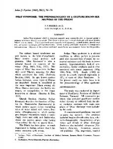
2.2 Williams-Otto Reactor Problem The reactor in the Williams-Otto plant [85], as modified by Roberts [72], will be used to illustrate the difficulties faced in RTO when the process model is subject to structural mismatch, and it will serve as a motivating example for the approaches studied in this thesis. Note that this reactor example has been used to illustrate model adequacy and RTO performance in numerous studies [34, 35, 89, 97]. 2.2.1 Description and Model Equations

FA ; XA,in = 1

FB ; XB,in = 1

TR

W

F = FA + FB XA , XB , XC , XE , XG , XP Fig. 2.1. Williams-Otto Reactor.

The reactor is illustrated in Figure 2.1. It consists of an ideal CSTR in which the following reactions occur:

26


A + B −→ C B + C −→ P + E C + P −→ G

k¯1 = 1.6599 × 106 e−6666.7/(TR +273.15) k¯2 = 7.2117 × 108 e−8333.3/(TR +273.15) k¯3 = 2.6745 × 1012 e−11111/(TR +273.15)

(2.18)

where the reactants A and B are fed with the mass flow rates FA and FB , respectively. The desired products are P and E. C is an intermediate product and G is an undesired product. The product stream has the mass flow rate F = FA + FB . Operation is isothermal at the temperature TR . The reactor mass holdup is W = 2105 kg. Simulated reality: Plant equations The steady-state model for the simulated reality results from the material balance equations: ¯ A − W r¯1 0 = FA − (FA + FB )X ¯ B − MB W r¯1 − W r¯2 0 = FB − (FA + FB )X MA ¯ C + MC W r¯1 − MC W r¯2 − W r¯3 0 = −(FA + FB )X MA MB M MP P ¯P + 0 = −(FA + FB )X W r¯2 − W r¯3 MB MC ¯ G + MG W r3 0 = −(FA + FB )X MC M M E E ¯E = ¯P + ¯G X X X MP MG with, ¯B , ¯AX r¯1 = k¯1 X

¯C , ¯B X r¯2 = k¯2 X

¯P ¯C X r¯3 = k¯3 X

¯ i : mass fraction of species i, Mi : molecular weight The variables are: X of species i. W : mass holdup. kj : kinetic coefficient of reaction j given in (2.18). In this example, the reaction scheme (2.18) corresponds to the simulated reality. However, since it is assumed that the reaction scheme is not well understood, the following two reactions have been proposed to model the system [35]: A + 2B −→ P + E A + B + P −→ G

k1 = η1 e−ν1 /(TR +273.15) k2 = η2 e−ν2 /(TR +273.15)

(2.19)

27

Two-reaction model: Model equations The steady-state model for the two-reaction approximation results from the material balance equations: 0 = FA − (FA + FB )XA − W r1 − W r2 MB MB 2W r1 − W r2 0 = FB − (FA + FB )XB − MA MA MP MP W r1 − W r2 0 = −(FA + FB )XP + MA MA ME 0 = −(FA + FB )XE + W r1 MA MG MG XE + XP XG = ME MP with, 2 r1 = k1 XA XB ,

r2 = k2 XA XB XP .

The kinetic coefficients k1 and k2 are given in (2.19). By assuming MA = MB = MP , all the molecular weight ratios that appear in the model equations are defined from the stoichiometry of the reactions. Process Measurements Forbes and Marlin [34] considered the process measurements yp = ¯ P F¯ )T . However, since in this work ¯G X ¯E X ¯C X ¯B X ¯A X (F¯B T¯R X measurement noise on the decision variables is not considered (the decision variables are assumed to be either setpoint values or known manipulated variables), the flow rates and reactor temperature are not considered as measurements. Also, the mass fraction of C is not included in the measurements since the presence of C is not assumed to be known, and it is not predicted by the model. Therefore, the ¯ P )T . ¯G X ¯E X ¯B X ¯A X measurement vector is chosen as yp = (X Nominal model parameters The four adjustable parameters θ = (η1 ν1 η2 ν2 )T are not identifiable from the process measurements yp . Two possible adjustable parameter sets where considered in [34]: in the first case, only the frequency

28


factors are updated (θ1 = (η1 η2 )T ), while in the second case, only the activation energies are updated (θ 2 = (ν1 ν2 )T ). Both sets are identifiable from the process measurements. Here, the first set θ1 = (η1 η2 )T is chosen. Typically, the fixed parameter values will be determined from detailed plant studies and/or engineering principles. In [34], the fixed parameters ν1 and ν2 were chosen such that the closed-loop RTO system converged to the same manipulated variable values for each adjustable set. In this work, the nominal values for the activation energies are the same as in [34], i.e., ν1 = 8077.6 K, and ν2 = 12438.5 K. 2.2.2 Optimization Problem The objective is to maximize the operating profit, which is expressed as the cost difference between the product and reactant flowrates: ¯ P F + 25.92X ¯ E F − 76.23FA − 114.34FB , (2.20) J(u, yp ) = 1143.38X which is equivalent to minimizing φ(u, yp ) = −J(u, yp ). The flowrate of reactant A (FA ) is fixed at 1.8275 kg/s. The flowrate of reactant B (FB ) and the reactor temperature (TR ) are the decision variables, thus u = (FB , TR )T . Plant optimum The optimal solution for the plant (simulated reality) is presented in Table 2.1. The mass fractions obtained at the optimal solution are given in Table 2.2. The profit surface is strictly convex for the operating range considered, and is presented in Figure 2.2. The profit contours are given in Figure 2.3. Table 2.1. Plant optimum

FB⋆

[kg/s] 4.787

TR⋆ [◦ C] 89.70

φ⋆real [$/s] 190.98

29

100

0

17

0

98

180

96

100 80 100 6

95 5.5

90

TR [°C]

5

85

4.5 80

F [kg/s] B

4

0 180

17

92

0

0

0

18

90

17

120

1

94

19

140

0

18 60

0

160

180

0 15

19

Reactor Temperature [°C]

Profit [$/s]

14

200

88 0

18

0

16

86

0

15

0

17

84 180

82

0

0

16

180

80 4

170

4.5

13

0 12 0 11

0

15

0

14

5

5.5

6

Reactant B Flow [kg/s]

Fig. 2.2. Plant profit surface

Fig. 2.3. Plant profit contours

Table 2.2. Plant mass fractions at the optimum

¯⋆ X A 0.08746

¯⋆ X B 0.38962

¯⋆ X C 0.015306

¯⋆ X E 0.10945

¯⋆ X G 0.10754

¯⋆ X P 0.29061

2.3 Classical Two-Step Approach to RTO 2.3.1 Principles The classical two-step approach implies an iteration between parameter estimation and optimization [20, 46, 63]. The idea is to estimate repeatedly the model parameters θ of the nonlinear steady-state model, and to use the updated model in the model optimization to generate new inputs. This way, the model is expected to represent the plant at its current operating point more accurately. The parameter estimation and optimization problems at the RTO iteration k are given next:

Parameter Estimation Step θ⋆k ∈ arg min with

θ id

J

J id := [yp (uk ) − y(uk , θ)]T R[yp (uk ) − y(uk , θ)],

(2.21)

30


Optimization Step u⋆k+1 ∈ arg min u

s.t.

Φ(u, θ⋆k ) := φ u, y(u, θ⋆k ) G(u, θ⋆k ) := g u, y(u, θ⋆k ) ≤ 0

(2.22)

uL ≤ u ≤ uU ,

Input Update uk+1 := (I − K)uk + Ku⋆k+1 k := k + 1

(2.23)

In the parameter estimation problem (2.21), uk are the inputs applied to the plant at the RTO iteration k and yp (uk ) are the plant measurements obtained at steady state. The solution to the parameter estimation problem are the parameters θ⋆k that are used to update the model in the next optimization problem. Given the solution to the optimization problem, u⋆k , the first-order exponential filter (2.23) is typically employed, for which K ∈ IRnu ×nu is a diagonal gain matrix with diagonal elements in the interval (0, 1]. The local stability of the two-step RTO system at the plant optimum is discussed in [34]. The RTO system of Figure 2.4 is stable at the plant optimum u⋆p for small perturbations in the inputs u if:

⋆

du dθ dyp

0,

where h is the step size and ej is the jth unit vector.

(2.37)

40


This approach requires nu perturbations to be carried out at each RTO iteration, and for each perturbation a new steady-state must be attained. If during the gradient evaluation, an important exogenous perturbation or a change in operating conditions takes place, the gradients estimated by this approach may become meaningless. 2.4.4 Dual ISOPE The idea behind dual ISOPE is to estimate the gradients based on the current and past operating points instead of perturbing each input individually at each iteration [12, 13]. This way, the total number of input changes required by the algorithm is expected to be less. The key issue is the ability to estimate experimental gradients reliably while updating the operating point. The input perturbations required in order to estimate the gradients might be suboptimal, and even infeasible in the presence of constraints. Indeed, there are two conflicting objectives: the “primal objective” consists in solving the optimization problem, while the “dual objective” aims at estimating accurate experimental gradients. These conflicting tasks can be accommodated by adding a constraint in the optimization problem so as to ensure sufficient information in the measurements and guarantee gradient accuracy. In [12, 13], a constraint that prevents ill-conditioning in gradient computation has been proposed. Given the current operating point, uk , the nu past operating points, uk−1 , . . . , uk−nu , and the corresponding measured plant output values, ∂y yp (uk ), yp (uk−1 ), . . . , yp (uk−nu ), an estimate of the gradient ∂up (uk ) can be obtained as follows [13]: ˆ := Y(uk ) U −1 (uk ) β k

(2.38)

with U(uk ) := [ uk − uk−1 . . . uk − uk−nu ] ∈ IRnu ×nu

(2.39) ny ×nu

Y(uk ) := [ yp (uk ) − yp (uk−1 ) . . . yp (uk ) − yp (uk−nu ) ] ∈ IR

(2.40)

Estimating the gradient from (2.38) requires the matrix U(uk ) to be non-singular. Furthermore, since the measurements yp are corrupted by measurement noise, it has been proposed in [12] to ensure that matrix U(uk ) is well-conditioned. In dual ISOPE algorithms, good

41

conditioning is achieved by introducing a lower bound on the inverse condition number of U(uk ): κ−1 (uk , uk−1 , . . . , uk−nu ) :=

σmin (U(uk )) ≥ ϕ, σmax (U(uk ))

(2.41)

where κ(uk , uk−1 , . . . , uk−nu ) is the condition number of U(uk ). The dual ISOPE algorithm can be summarized as follows [13]: 1. Select an initial point u0 and nu additional points u−nu , u−nu +2 , . . . , u−1 such that the matrix U(u0 ) is sufficiently well conditioned. Initialize the parameters of the algorithm, i.e. K, ϕ and the parameter ǫ corresponding to the termination criterion kuk+1 − uk k ≤ ǫ. Apply the points u−nu , u−nu +2 , . . . , u−1 to the plant and measure the plant outputs yp (uj ), yp (u−nu +2 ), . . . , yp (u−1 ) at steadystate. Set k = 0. 2. Apply uk to the plant and measure yp (uk ) at steady-state operˆ according to ation. Obtain an estimate of the plant gradient β k (2.38). 3. Update the model parameters θk by solving a parameter estimation problem with the constraint of matching the plant and model outputs at uk (see output-matching requirement (2.33)). 4. Compute the ISOPE modifier λk as: ∂y ∂φ ˆ u , y(u , θ ) β − (u , θ ) , (2.42) λT := k k k k k k k ∂y ∂u and solve the following modified optimization problem including the conditioning constraint: u⋆k+1 ∈ arg min φ(u, y(u, θk )) + λT ku u

(2.43)

−1

s.t. κ (¯ u, uk , . . . , uk−nu +1 ) ≥ ϕ, ¯ = (I − K)uk + Ku, u uL ≤ u ≤ uU ,

5. Set uk+1 := (I − K)uk + Ku⋆k+1 . If kuk+1 − uk k ≤ ǫ, terminate. Else, set k := k + 1 and return to Step 2. ¯ corresponds to the filtered value of the Notice that in (2.43) u input.

42


Example 2.2 Consider a two-dimensional optimization problem (nu = 2). The left-side plot of Figure 2.12 uses the past operating points uk = [0 − 0.5]T and uk−1 = [0 0.5]T , while the right-side plot uses the past operating points uk = [0 − 0.1]T and uk−1 = [0 0.1]T . The conditioning constraint κ−1 (u, uk , uk−1 ) can be evaluated in terms of the location of the new operating point u = [u1 u2 ]T . The contour levels corresponding to values of κ−1 of 0.1, 0.2, 0.3 and 0.4 are represented.

1.5

1.5 0.1

1

1 0.3

0. 3

0.5

0. 4

0.3

0.4

0.1

3

4

−0.5

3

0.

0.

−0.5

0 0.1

u2

0. 1

0.4

0 0.

1 0.

0.3

0.5

u2

0.2

0.1

0.2

0.3

−1

0.2

0.1

−1.5 −2

0.2

0.2

0.1

−1

0.2

−1.5

−1

−0.5

0

u1

0.5

1

1.5

2

−1.5 −2

−1.5

−1

−0.5

0

u1

0.5

1

1.5

2

Fig. 2.12. Contour maps for the conditioning constraint (2.41) for two cases of previous points (more distant on the left and closer on the right).

The conditioning set D(u, uk , uk−1 ) is defined as: o n σmin (U(u)) ≥ϕ , D(u, uk , uk−1 ) := u ∈ IRnu : σmax (U(u))

The geometric characterisation of the set D has been analyzed in [13, 81] for the two-dimensional case. It consists of two discs of the same radius r, located symmetrically with respect to the line defined by the points uk and uk−1 . The discs are centered at a distance hd from the centroid of the points uk and uk−1 , in a direction orthogonal to the line defined by uk and uk−1 , with 1 − ϕ2 kuk − uk−1 k 4ϕ 1 + ϕ2 kuk − uk−1 k hd = 4ϕ

r=

Finally, not mentioned in [13, 81] but of the greatest importance is the scaling of the input variables, since the conditioning set D will completely depend on this scaling.

3 Real-Time Optimization via Constraint Adaptation

In the presence of uncertainty, the constraints predicted by the model do not quite match the actual constraints of the plant. This chapter investigates a so-called constraint-adaptation algorithm, which uses measurements for adapting the process constraints while relying on a fixed process model for satisfying the remaining parts of the NCO. The idea behind constraint adaptation is to use measurements of the constraints for modifying the constraints in the optimization problem between successive RTO periods so as to track the actual constraint values. This way, constraint adaptation guarantees that a feasible, yet suboptimal, operating point is attained upon convergence. Suboptimality will depend on how well the process model predicts the gradient of the cost function and of the active constraints. In addition to the constraint modifiers used in constraint adaptation, the full modifier-adaptation scheme studied in Chapter 4 also makes use of modifiers for the cost and constraint gradients in order to enforce optimality. Despite being a subproblem of modifier-adaptation, constraint adaptation deserves to be studied on its own because of its simplicity, as it does not require that the gradient of the cost and constraint functions be estimated experimentally, and also because it can provide a satisfactory solution for a large number of optimization problems for which most of the optimization potential lies in keeping the correct set of constraints active. Although constraint adaptation converges to a feasible operating point, the constraints can be violated during steady-state operation at the operating points produced by the algorithm prior to convergence, or during the dynamic response between successive steady-state operating points. A convenient way to avoid these infeasibilities is by means

44

Chapter 3: Constraint Adaptation

of model predictive control (MPC) tailored to control the constraints. Section 3.3 presents an approach for integrating constraint adaptation with MPC. The applicability and suitability of constraint adaptation is demonstrated through the case study of a solid-oxide fuel cell (SOFC) system in Subsection 3.3.3.

3.1 Variational Analysis of NCO in the Presence of Parametric Uncertainty Satisfying the NCO is necessary for process operation to be feasible and achieve optimal performance. More precisely, failure to meet any of the primal feasibility conditions (2.5) leads to infeasible operation, whereas violating the complementarity and dual feasibility conditions (2.6-2.8) results in suboptimal operation. That is, a very desirable property for a RTO scheme is that the iterates converge to a point at which the NCO of the real process are satisfied. Regarding fixed-model RTO methods, the algorithm described in [37], provided it converges, can be shown to attain such points. However, for RTO schemes to satisfy certain NCO, it is necessary that the gradients of the cost and constraint functions be available, which in turn requires that these gradients be estimated experimentally from the available measurements. In this section, we conduct a variational analysis of the NCO in the presence of uncertainty. The underlying idea is to quantify how deviations of the parameters θ from their nominal values θ◦ affect the NCO and, through them, the performance of the process. Said differently, the objective is to determine which parts of the NCO influence the process performance the most, and which parts can be dropped without much impact in terms of performance. For simplicity, and without loss of generality, the bound constraints uL ≤ u ≤ uU shall be dropped, and only the general inequality constraints G(u, θ) ≤ 0 shall be considered for this analysis.1 In this section, a minimizing solution of Problem (2.3) will be denoted by u⋆θ when we need to emphasize the dependency on θ. Also, we shall assume, without loss of generality, that all the constraints G(·, θ ◦ ) are active at u⋆θ◦ , since an inactive constraint at u⋆θ◦ can always be removed from Problem (2.3). The number of active constraints 1

Alternatively, just replace G(u, θ) ≤ 0 by the general constraints z(u, θ) ≤ 0 defined in (2.10).

45

at an optimal solution point being less than the number of input variables, there exist directions in the input space along which taking an infinitesimal step from an optimal solution point does not modify the active constraints. A characterization of these directions is given in the next definition. Definition 3.1 (Constraint-Seeking and Sensitivity-Seeking Directions) If the assumptions of Theorem 2.3 are met, the Jacobian ⋆ matrix ∂G ∂u is full rank at (uθ ◦ , θ ◦ ). Singular value decomposition of ∂G ∂u gives ∂G ⋆ T ∂u (uθ ◦ , θ ◦ ) := U Σ V , where Σ is a (ng × nu ) matrix of the form   σ1 0 ··· 0  .. . . ..  := Σ c 0 ; .. Σ =  . . . . σng 0 · · · 0

U is an (ng × ng ) orthonormal matrix; and V := [ Vc Vs ] is an (nu × nu ) orthonormal matrix. The ng columns of Vc define the constraint-seeking directions, while the (nu − ng ) columns of Vs define the sensitivity-seeking directions. Clearly, infinitesimal moves along a constraint-seeking direction away from an optimal solution point modify the active constraint values, whereas infinitesimal moves along a sensitivity-seeking direction leave the active constraints unchanged. The subsequent theorem quantifies the variation of the optimal inputs, in both the constraint- and sensitivity-seeking directions, which is induced by a deviation of the model parameters from their nominal values. Theorem 3.1 (Input Variations in the Constraint-Seeking and Sensitivity-Seeking Directions) Let the assumptions in Theorem 2.3 be met and η be chosen such that Theorem 2.3 applies. Let δu⋆ := u⋆θ − u⋆θ◦ denote the variation of the optimal inputs induced by the variation δθ := θ − θ◦ , with θ ∈ Bη (θ ◦ ), and consider the variations δuc and δus of the optimal inputs in the constraint-seeking and sensitivity-seeking directions, respectively, c c s T ⋆ δu δu . s := V V δu

46


Then, the first-order approximations of δuc and δus are given by: δuc = − δus = −

∂G c −1 ∂G ∂u V ∂θ δθ + o(kδθk) −1 h 2 2 2 ∂ L Vs T ∂∂uL2 Vs − ∂∂uL2 Vc Vs T ∂θ∂u

(3.1) ∂G ∂u V

+ o(kδθk), 2

2

∂ L , where ∂∂uL2 , ∂θ∂u point θ = θ ◦ .

∂G ∂u

and

∂G ∂θ

c −1

∂G ∂θ

i

δθ (3.2)

are calculated at the nominal solution

Proof. By Theorem 2.3, there exist continuously differentiable vector functions u⋆θ and µ⋆θ satisfying the second-order sufficient conditions for a local minimum of Problem (2.3) for each θ ∈ Bη (θ◦ ). The active constraints being linearly independent, and all the inequality constraints being assumed active with strictly positive Lagrange multipliers, we have G(u⋆θ , θ) = 0 ∂L ⋆ ⋆ ∂u (uθ , µθ , θ)

=

(3.3)

∂Φ ⋆ ∂u (uθ , θ)

+

⋆ µ⋆θ T ∂G ∂u (uθ , θ)

= 0,

(3.4)

for each θ ∈ Bη (θ◦ ). The primal feasibility condition (3.3) gives 0 = G(u⋆θ , θ) − G(u⋆θ◦ , θ◦ ) =

=

∂G ⋆ ∂θ (uθ◦ , θ ◦ ) ∂G ⋆ ∂θ (uθ◦ , θ ◦ )

δθ + δθ +

∂G ⋆ ∂u (uθ ◦ , θ ◦ ) ∂G ⋆ ∂u (uθ ◦ , θ ◦ )

δu⋆ + o(kδθk) Vc δuc +

∂G ⋆ ∂u (uθ◦ , θ ◦ )

Vs δus

+ o(kδθk). ∂G c s c Then, (3.1) follows by noting that ∂G ∂u V = 0 and ∂u V = UΣ is ⋆ nonsingular at θ = θ◦ , provided that uθ◦ is a regular point for the active constraints. On the other hand, the dual feasibility condition (3.4), taken along the sensitivity-seeking directions, gives

0 = Vs T = Vs T

∂L

⋆ ⋆ ∂u (uθ , µθ , θ)

h

−

T ∂L ⋆ ⋆ ∂u (uθ ◦ , µθ ◦ , θ ◦ )

∂2L ⋆ ⋆ ∂θ∂u (uθ ◦ , µθ ◦ , θ ◦ )

2

δθ + ∂∂uL2 (u⋆θ◦ , µ⋆θ◦ , θ◦ ) δu⋆ i ∂2L (u⋆θ◦ , µ⋆θ◦ , θ◦ ) δµ⋆ + o(kδθk), + ∂µ∂u

47 2

∂ L s T = [ ∂G where δµ⋆ := µ⋆θ − µ⋆θ◦ . Since Vs T ∂µ∂u ∂u V ] = 0, at θ = θ ◦ , 2 we obtain h 2 i 2 2 ∂ L 0 = Vs T ∂θ∂u δθ + ∂∂uL2 Vc δuc + ∂∂uL2 Vs δus + o(kδθk), (3.5)

and from (3.1), h 2 ∂ L − 0 = Vs T ∂θ∂u + o(kδθk).

∂2L c ∂u2 V

∂G c −1 ∂G ∂u V ∂θ

i

2 δθ + Vs T ∂∂uL2 Vs δus 2

Finally, (3.2) follows by noting that V s T ∂∂uL2 Vs is nonsingular at θ = θ◦ , provided that the second-order sufficient conditions for a local minimum of Problem (2.3) for θ◦ hold at u⋆θ◦ . 2 In the presence of uncertainty, i.e., when the model parameters θ deviate from their nominal values θ◦ , failure to adapt the process inputs results in the cost value Φ(u⋆θ◦ , θ). To combat uncertainty, adaptation of the process inputs can be made both in the constraintand the sensitivity-seeking directions. The cost value corresponding to perfect input adaptation in the constraint-seeking directions is Φ(u⋆θ◦ + Vc δuc , θ), whereas perfect input adaptation in the sensitivityseeking directions gives Φ(u⋆θ◦ +Vs δus , θ). The cost variations δΦc and δΦs obtained upon adaptation of the process inputs in the constraintand sensitivity-seeking directions, respectively, are thus given by δΦcθ := Φ(u⋆θ◦ + Vc δuc , θ) − Φ(u⋆θ◦ , θ),

δΦsθ := Φ(u⋆θ◦ + Vs δus , θ) − Φ(u⋆θ◦ , θ). Approximations of these variations are derived in the following theorem, based on the first-order approximations of the directional input variations established in Theorem 3.1. Theorem 3.2 (Cost Variations in the Constraint-Seeking and Sensitivity-Seeking Directions) Let the assumptions in Theorem 2.3 hold and η be chosen such that Theorem 2.3 applies. Then, the first- and second-order approximations of the cost variations δΦcθ and δΦsθ , for θ ∈ Bη (θ ◦ ), are given by 2

For the sake of conciseness, the arguments u⋆θ ◦ , µ⋆θ ◦ , θ ◦ are dropped in the remainder of the proof.

48


δΦcθ = µ⋆θ◦ T ∂G ∂θ δθ + o(kδθk) δΦsθ δθ

T

= h

(3.6)

2 2 ∂2 L 1 ∂2L s s T ∂ 2 L s −1 (Vs T ∂∂uΦ2 Vs )(Vs T ∂∂uL2 Vs )−1 Vs T ∂θ∂u 2 ∂u∂θ V (V ∂u2 V )

− δθ T

h

∂2Φ s s T ∂ 2 L s −1 s T ∂ 2 L V ∂θ∂u ∂u∂θ V (V ∂u2 V ) 2

2

∂ Φ ∂ L where ∂G ∂θ , ∂u2 , ∂u2 , solution point θ = θ ◦ .

∂2 Φ ∂u∂θ ,

and

∂2L ∂u∂θ

i

δθ + o(kδθk2 ),

i

δθ

(3.7)

are calculated at the nominal

Proof. Consider the variation in cost function δΦθ := Φ(u⋆θ , θ) − Φ(u⋆θ◦ , θ). Its approximation up to second-order reads δΦθ =

T ∂2 Φ ∂Φ ⋆ ⋆ ⋆ ⋆ ∂u (uθ ◦ , θ ◦ ) δu + δθ ∂u∂θ (uθ◦ , θ ◦ ) δu 2 + 21 δu⋆ T ∂∂uΦ2 (u⋆θ◦ , θ◦ ) δu⋆ + o(kδθk2 ),

where δθ := θ−θ◦ and δu⋆ := u⋆θ −u⋆θ◦ .3 Splitting the input variations δu⋆ into constraint- and sensitivity-seeking directions, and noting that ∂Φ s ∂u V = 0 at θ = θ ◦ , we obtain δΦθ =

T ∂2Φ T ∂2Φ ∂Φ c c c c s s ∂u V δu + δθ ∂u∂θ V δu + δθ ∂u∂θ V δu 2 2 + 21 δuc T Vc T ∂∂uΦ2 Vc δuc + 21 δus T Vs T ∂∂uΦ2 Vs δus 2 + δuc T Vc T ∂∂uΦ2 Vs δus + o(kδθk2 ).

(3.8)

On the one hand, the cost variation δΦcθ is obtained by letting δus = 0 in (3.8), and dropping the second-order terms, δΦcθ =

∂Φ c c ∂u V δu

+ o(kδθk)

From (3.1), we then get δΦcθ = −

∂Φ c ∂u V

∂G c −1 ∂G ∂u V ∂θ

δθ + o(kδθk).

c ∂G c −1 (dual feaand (3.6) follows by noting that µ⋆θ◦ T = −( ∂Φ ∂u V )( ∂u V ) sibility condition along constraint-seeking directions). On the other hand, the cost variation δΦsθ is obtained by letting c δu = 0 in (3.8), 3

For sake of conciseness, the arguments u⋆θ ◦ , θ ◦ are dropped in the remainder of the proof.

49 2

2

∂ Φ s V δus + 21 δus T Vs T ∂∂uΦ2 Vs δus + o(kδθk2 ), δΦsθ = δθ T ∂u∂θ

and (3.7) follows upon substitution of δus = 2 2 T T s ∂ L s −1 s ∂ L −(V ∂u2 V ) V ∂θ∂u δθ + o(kδθk), as obtained from (3.5) with δuc = 0. 2 Overall, the variational analysis shows that failure to adapt the process inputs in the constraint-seeking directions results in cost variations in the order of the error δθ; moreover, constraint violation can occur if the constraint-seeking directions are not adapted. On the other hand, failure to adapt the process inputs in the sensitivity-seeking directions gives cost variations proportional to the squared error δθ2 only. From a practical perspective, and provided that model mismatch remains moderate, more effort should therefore be placed on satisfying the process constraints rather than the sensitivity part of the NCO. Based on these considerations, an algorithm implementing constraints adaptation is presented in the following section.

3.2 Constraint Adaptation 3.2.1 Principles of Constraint Adaptation The adaptation of additive constraint modifiers corresponds to the “classical” constraint-adaptation scheme [17, 33]. The constraints are corrected by simply offsetting the constraint predictions as G(u, θ) + ε ≤ 0,

(3.9)

where ε ∈ IRng denotes the vector of the constraint correction factors or modifiers. The decision variables are updated in each RTO iteration by solving an NLP problem similar to (2.3), which takes the constraint corrections into account: u⋆k+1 ∈ arg min Φ(u, θ) u

(3.10)

s.t. G(u, θ) + εk ≤ 0 uL ≤ u ≤ uU .

Next, the optimal solution point u⋆k+1 is applied directly to the plant:

50

Chapter 3: Constraint Adaptation min

Φ(u, θ)

u

uk+1

s.t. G(u, θ) + εk ≤ 0 uL ≤ u ≤ uU

6 εk

G(uk+1 , θ)

k ←k+1

6 εk+1 adapt.

- ?Gp (uk+1 )

j

Nominal model Real process

Fig. 3.1. Recursive adaptation of additive constraint modifiers.

uk+1 = u⋆k+1 Then, assuming that measurements are available for every constrained quantity at each RTO iteration, the constraint modifiers can be updated recursively as εk+1 = εk − B [G(uk+1 , θ) + εk − Gp (uk+1 )] ,

(3.11)

where B ∈ IRng ×ng is a gain matrix. On the other hand, the model parameters θ are kept constant at their nominal values. Note that (3.11) can also be written as εk+1 = (I − B)εk + B (Gp (uk+1 ) − G(uk+1 , θ)) ,

(3.12)

which makes explicit the exponential filtering effect of B. In the special case where B is a diagonal matrix with entries bi , i = 1, . . . , ng , the update law can be seen as the filtered difference Gp,i (uk+1 ) − Gi (uk+1 , θ) between the predicted and measured values of each constraint. No adaptation is performed for the ith constraint by setting bi = 0, whereas no filtering is used for this constraint when bi = 1, i.e., the full correction Gp,i (uk+1 ) − Gi (uk+1 , θ) is applied. The proposed constraint-adaptation algorithm is illustrated in Figure 3.1. Note that, unlike many other existing RTO schemes, the present approach relies on constraint measurements only, and it does not require that the gradient of the cost and constraint functions be estimated. In return, of course, the constraint-adaptation algorithm

51

may terminate at a suboptimal, yet feasible, point upon convergence. The extent of this loss of optimality is determined by the quality of the process model. It may happen that some of the constraints are not measured during process operation, especially in those applications having very many constraints. In this case, observers that estimate the values of the unmeasured constrained quantities based on the available measurements (e.g., measured outputs yp ) can be used. To avoid potential conflicts between the control and estimation tasks, however, great care must be taken to ensure that the rate of convergence of these observers is actually much faster than the RTO execution period itself. Furthermore, if the unmeasured constrained quantities cannot be estimated from plant measurements, one should opt for a more conservative approach, e.g., a robust optimization approach [96]. It is also possible to impose permanent (conservative) constraint backoffs to the unmeasured constraints [54]. The computational complexity of the NLP problems in constraint adaptation is similar to that of the classical two-step approach. Constraint adaptation is in fact less computationally demanding since it does not require the solution of a parameter estimation problem at each iteration. 3.2.2 Constraint-Adaptation Algorithm We start the analysis with a number of definitions relative to the parametric programming problem (3.10) [6, 31]. The feasible solution map, U (·), is defined as U (ε) := {u ∈ [uL , uU ] : G(u, θ) + ε ≤ 0}, such that, for each ε ∈ IRng , U (ε) is a subset of IRnu . A straightforward property of feasible solution sets is U (ε1 ) ⊂ U (ε2 ),

if ε1 ≥ ε2 .

Observe also that U (ε) may be empty for some values of ε, which motivates the definition of the domain of U (·) as dom U := {ε ∈ IRng : U (ε) 6= ∅}.

52


Clearly, ε2 ∈ dom U for every ε2 ≤ ε1 provided that ε1 ∈ dom U . In turn, the optimal value function, Φ⋆ (·), and the optimal solution map, U ⋆ (·), are defined as inf{Φ(u, θ) : u ∈ U (ε)}, if ε ∈ dom U ⋆ Φ (ε) := +∞, otherwise U ⋆ (ε) :={u ∈ U (ε) : Φ(u, θ) = Φ⋆ (ε)}.

The cost function Φ(·, θ) being continuous and the feasible region U (ε) being bounded, it follows that the infimum Φ⋆ (ε) is assumed somewhere on [uL , uU ] for each ε ∈ dom U , thus being a minimum (Weierstrass’ theorem – see, e.g., [7], Theorem 2.3.1). Besides the existence of a minimum point, we make the following uniqueness assumption throughout. Assumption 3.1 Let θ be given. For each ε ∈ dom U , Problem (3.10) has a unique (global) solution point. This assumption implies that U ⋆ (ε) is a singleton, for each ε ∈ dom U . That is, at any RTO iteration k, we have u⋆k+1 = U ⋆ (εk ), if εk ∈ dom U . Also, the map Γ : dom U → IRng representing the difference between the process constraints and the corrected values of the predicted constraints for a given correction ε, Γ(ε) := G(u, θ) + ε − Gp (u),

u = U ⋆ (ε),

(3.13)

is a point-to-point map. Remark 3.1 In the more general case where Assumption 3.1 does not hold, U ⋆ (ε) may not be a singleton for ε ∈ dom U . That is, (4.15) ng defines a point-to-set map [45], Γ : dom U → 2IR . Based on the foregoing definitions and Assumption 3.1, the (additive) constraint-adaptation algorithm M can be stated as εk+1 = M(εk ),

(3.14)

M(ε) := ε − B Γ(ε),

(3.15)

where

for any ε ∈ dom U .

53

3.2.3 Feasibility An important property of the constraint-adaptation algorithm M is that the iterates, upon convergence (in the absence of measurement noise and process disturbances), are guaranteed to terminate at a feasible point, under mild conditions. This is formalized in the following theorem: Theorem 3.3 (Feasibility upon Convergence) Let the gain matrix B be nonsingular, and assume that the constraint-adaptation algorithm M converges, with limk→∞ εk = ε∞ . Then, u∞ = U ⋆ (ε∞ ) is a feasible operating point. Proof. Since B is nonsingular, every fixed point ε◦ of the algorithmic map M(·) must satisfy Γ(ε◦ ) = G(u◦ , θ) + ε◦ − Gp (u◦ ) = 0, where u◦ = U ⋆ (ε◦ ). In particular, ε∞ being a fixed point of M(·), we have Gp (u∞ ) = G(u∞ , θ) + ε∞ ≤ 0, with u∞ = U ⋆ (ε∞ ).

2

For certain problems, the iterates may converge by following an infeasible path (i.e., with violation of the constraints), even though the constraint-adaptation algorithm starts at a feasible point. A way of reducing the maximum violation of a given constraint, say Gp,i , is by decreasing the corresponding filter parameter bi (in the case where B is a diagonal matrix). Yet, this is at the expense of a slower convergence rate. Even though the iterates may follow an infeasible path, a straightforward corrolary of Theorem 3.3 is that the constraint-adaptation algorithm, provided it converges, can yield feasible operation after a finite number of RTO periods upon backing-off the constraints of the original RTO problem. 3.2.4 Active Set Owing to the importance of constraints in optimization problems, a very desirable property of any RTO scheme is the capability of detecting the optimal set of active constraints. Since the constraintadaptation algorithm approximates the actual gradients of the cost

54


Table 3.1. Values of the uncertain parameters θ in Problem (3.16) corresponding to the model and two simulated realities for the plant.

θ1 θ2 θ3

Model Plant A Plant B 0.75 0.75 0.75 1.40 2.00 2.00 1.00 1.00 1.80

and constraint functions by using a fixed process model, it cannot be guaranteed that a point satisfying the complementarity slackness and dual feasibility conditions (2.6–2.8) is attained. Observe, however, that the active set determined by the process model is known to be the same as the actual optimal active set, provided that the model mismatch remains moderate (see Theorem 2.3). There is therefore much hope that the constraint-adaptation algorithm can provide a good approximation of the correct active set, even in the case of large model mismatch. These important considerations are illustrated next through a numerical example; they are further illustrated by the case study application presented in Subsection 3.2.8. Example 3.1 Consider the following quadratic program (QP): min Φ(u, θ) := (u1 − θ1 )2 + (u2 − θ1 )2

s.t.

(3.16)

G1 := u1 − θ2 (1 − u2 ) ≤ 0 G2 := u2 θ3 − 2(1 − u1 ) ≤ 0,

with two decision variables u = [u1 u2 ]T , three model parameters θ = [θ1 θ2 θ3 ]T , and two inequality constraints. The parameter values θ for the model and the simulated realities A and B for the plant are reported in Table 3.1. We start by considering the plant A. Since the parameters θ1 and θ3 are identical in the model and the plant, no adaptation is needed for G2 (i.e., ε2 = 0); however, this information is not known by the constraint-adaptation algorithm. Furthermore, the cost functions of the model and the plant are identical, i.e., Φ(u, θ) ≡ Φp (u). Hence, the only uncertainty is in the constraint G1 . Upon application of the constraint-adaptation algorithm M with B = I2×2 and ε0 = [0 0]T , the iterates converge to the fixed point ε∞ = [− 51 0]T . The correspond-

55

Plant A 0.9

0.9

0.8

0.8

0.7

0.7

0.6

P=C

u2

u2

P

0.6

M

0.5

M

0.5

0.4

0.4 0.4

0.5

0.6

u1

0.7

0.8

0.9

0.4

0.5

0.6

u1

0.7

0.8

0.9

0.7

0.8

0.9

Plant B

0.8

0.8

0.7

0.7

u2

0.9

u2

0.9

0.6

0.6

M

P 0.5

C

M

P

0.5

0.4

0.4 0.4

0.5

0.6

u1

0.7

0.8

0.9

0.4

0.5

0.6

u1

Fig. 3.2. Illustration of the constraint-adaptation algorithm for Problem (3.16). Left plots: no constraint adaptation; Right plots: converged constraint adaptation; Thin solid lines: constraint bounds for the plant; Colored area: feasible region; Thick dash-dotted lines: constraint bounds predicted by the model without adaptation; Thick solid lines: constraint bounds predicted by the model upon convergence of the constraintadaptation algorithm; Dotted lines: contours of the cost function; Point P: optimum for the plant; Point M: optimum for the model without adaptation; Point C: optimum for model upon convergence of the constraint-adaptation algorithm; Arrows: direction of constraint adaptation.

ing operating point u∞ lies at the intersection of the constraints Gp,1 and Gp,2 (see Figure 3.2, Plant A). Note that the correct optimal point would also be found in the case where θ1 6= θ 1 , as long as both inequality

56


constraints remain active at this point. In the plant B, both the constraints G1 and G2 are uncertain. Observe that adaptation is absolutely warranted in this scenario, since the solution of the model-based optimization problem (3.16) leads to infeasible operation. The constraint69 14 T adaptation algorithm converges to the fixed point ε∞ = [− 290 29 ] , with the same initial guess and gain matrix as previously. The corresponding operating point lies on the constraint G2 at the point of tangency with the cost contours, while the constraint G1 is inactive. Here again, the correct active set is detected upon convergence of the constraint-adaptation algorithm, yet the iterates converge to a suboptimal point (see Figure 3.2, Plant B). The loss of performance, around 7%, is due to the error made in evaluating the gradient of the active constraint G2 . This loss is rather limited in view of the substantial variation in the model parameters θ2 and θ3 . 3.2.5 Convergence A particularly important aspect of any RTO scheme relates to its convergence properties. It has been shown earlier that, upon convergence, the constraint-adaptation algorithm M terminates at a feasible operating point, under mild conditions. Yet, this algorithm may not systematically converge. For example, it may happen that the NLP problem (3.10) becomes infeasible because a coefficient of the constraint modifiers ε has grown too big. It can also happen that a coefficient of the constraint modifiers oscillates between two values because the corresponding filter parameter is too large. In the absence of measurement noise and process disturbances, the following theorem provides a necessary condition for the convergence of M to a fixed point, and it establishes the convergence rate. Theorem 3.4 (Necessary Condition and Convergence Rate) Let ε∞ be a fixed point of the constraint-adaptation algorithm M, and assume that: 1. the second-order sufficient conditions for a local minimum of Problem (3.10) with ε = ε∞ hold at u∞ = U ⋆ (ε∞ ), with the associated L Lagrange multipliers µ∞ , ζ U ∞ , and ζ ∞ ; 2. u∞ is a regular point for the active constraints, i.e. LICQ holds; L U > 0 for each active constraint, i.e. 3. µi,∞ > 0, ζi,∞ > 0, and ζi,∞ strict complementary slackness holds.

57

Then, a necessary condition for the local convergence of M to the fixed-point ε∞ is that the gain matrix B be chosen such that io n h ∂G −1 < 1, (3.17) (u , θ) P M N ̺ I − B I + ∂up (u∞ ) − ∂G ∞ u ∞ ∞ ∂u where the matrices M∞ ∈ IR(ng +3nu )×(ng +3nu ) , N∞ ∈ IR(ng +3nu )×ng , and Pu ∈ IRnu ×(ng +3nu ) are defined as M∞ := 

∂2L ∂u∂u ∂G µ1,∞ ∂up,1

   ..   .  ∂Gp,ng µ  ng ,∞ ∂u  diag(ζ U )

∂Gp,1 T ∂u

Gp,1

··· ..

∂Gp,ng T ∂u

Pu :=

−Inu ×nu

. Gp,ng diag(u − uU )

∞ − diag(ζ L∞ )

N∞ :=

Inu ×nu

diag(uL − u)

0ng ×nu − diag(µ∞ ) 0ng ×2nu Inu ×nu 0nu ×(ng +2nu ) ,

T

         

(u∞ )

,

and ̺{·} stands for the spectral radius. Moreover, if the constraint adaptation converges, then the rate of convergence is linear. Proof. It follows from the assumptions and Theorem 2.3 that there is some η > 0 such that, for each ε ∈ Bη (ε∞ ), there exists a unique continuously differentiable vector function u⋆ = U ⋆ (ε) satisfying the second-order sufficient conditions for a local minimum of Problem (3.10), with u∞ = U ⋆ (ε∞ ). Moreover, we have (see Theorem 2.3): ∂U ⋆ ∂ε (ε∞ )

= −Pu M−1 ∞ N∞ .

The constraint functions Gi (·, θ) and Gp,i (·), i = 1, . . . , ng , being differentiable with respect to u, it follows that Γ(·) given by (3.13) is itself differentiable with respect to ε in a neighborhood of ε∞ , and we have ⋆ ∂Gp ∂Γ ∂G ∂U ∂ε (ε∞ ) = I − ∂u (u∞ ) − ∂u (u∞ , θ) ∂ε (ε∞ ) ∂G −1 = I + ∂up (u∞ ) − ∂G ∂u (u∞ , θ) Pu M∞ N∞ .

58


That is, a first-order approximation of Γ in a neighborhood of ε∞ is i h ∂G −1 Γ(ε) = I + ∂up (u∞ ) − ∂G ∂u (u∞ , θ) Pu M∞ N∞ δε + o(kδεk),

where δε := ε − ε∞ . Next, suppose that the algorithm (3.14), with ε0 given, converges to ε∞ . Then, ∃k0 > 0 such that εk ∈ Bη (ε∞ ), ∀k > k0 ,

and we have δεk+1 = ΥG ∞ δεk + o(kδεk k), for each k > k0 , with h ∂Gp := I − B I + ΥG ∞ ∂u (u∞ ) −

∂G ∂u (u∞ , θ)

i . Pu M−1 N ∞ ∞

(3.18)

(3.19)

For M to converge to ε∞ , the spectral radius of ΥG ∞ must therefore be less than 1. Finally, it follows from (3.18) that, if M converges, then it has a linear rate of convergence. 2 Remark 3.2 It follows from the local analysis performed in the proof of Theorem 3.4 that a necessary condition for the iterates εk to converge to the fixed point ε∞ monotonically, i.e. without oscillations around ε∞ , is that all the eigenvalues of matrix ΥG ∞ be nonnegative. We illustrate these results in the following example. Example 3.2 Consider the QP problem (3.16) of Example 3.1, with the parameters specified in Table 3.1. For the plant A, the converged constraint modifiers as well as the corresponding inputs and multipliers are: 5 2 1 −5 ⋆ 3 54 , µ (ε ) = . , u⋆ (ε∞ ) = ε∞ = ∞ 2 1 0 3 27

In particular, it can be verified that the second-order sufficient condi⋆ ∂Γ tions hold at u⋆ (ε∞ ). The derivatives ∂u ∂ε and ∂ε at ε∞ are obtained as 5 1 ∂Γ ∂u⋆ 1 − 95 79 3 −3 , . (ε∞ ) = (ε ) = ∞ 10 5 − 0 1 ∂ε 9 ∂ε 9 9

59

Upon choosing the diagonal gain matrix as B := bI, the matrix ΥG ∞ reads 1 − 53 b 31 b . ΥG ∞ = 0 1−b Clearly, the necessary condition (4.55) is satisfied for every 0 < b < 65 . Note also that monotonic convergence is ensured as long as 0 < b ≤ 35 (see Remark 3.2). The foregoing analysis provides conditions that are necessary for the constraint-adaptation algorithm to converge. Yet, these conditions are inherently local and, in general, are not sufficient for convergence. This is the case, e.g., when the algorithm starts far away from a fixed point. Another source of divergence for the constraint-adaptation algorithm is when the constraint map Γ(ε) is always nonzero, i.e., the algorithm does not have a fixed point. One such example is discussed subsequently. Table 3.2. Values of the uncertain parameters θ in Problem (3.20) corresponding to the model and the plant.

θ1 θ2 θ3

Model Plant 0.5 0.5 1.1 0.2 1.0 -1.0

Example 3.3 Consider the convex QP: min Φ(u, θ) = (u1 − θ1 )2 + (u2 − θ1 )2 u≥0

s.t.

(3.20)

G := θ2 − u1 − u2 θ3 ≤ 0

with two decision variables u = [u1 , u2 ], three uncertain parameters θ = [θ1 , θ2 , θ3 ] whose values corresponding to the model and the plant are given in Table 3.2, and a single constraint to be adapted using the constraint modifier ε. Upon application of the constraint-adaptation algorithm with a scalar gain b > 0, the iterates are found to diverge, εk → +∞ as

60


k → +∞. The situation is illustrated in the left plot of Figure 3.3. Here, divergence results from the fact that the optimal solution set U ⋆ (ε) does not intersect the plant feasible region, irrespective of the constraint modifier ε. That is, the constraint map Γ (ε) shown in the right plot of Figure 3.3 is always nonzero. Clearly, the necessary conditions given in Theorem 3.4 do not hold for this problem.

2

u1 ⋆ = u2 ⋆

1

0.8

0.6

1 0.5 0 −2

M

u2

1.5

−1

0

1

2

0

1

2

ε

0

0.4

P Γ (ε)

−0.5

0.2

−1 −1.5 −2

0 0

0.2

0.4

u1

0.6

0.8

1

−2.5 −2

−1

ε

Fig. 3.3. Divergence of the constraint-adaptation algorithm for Problem (3.20). Left plot: iterates in the u1 -u2 space; Thin solid lines: constraint bounds for the plant; Colored Area: feasible region; Thick dash-dotted lines: constraint bounds predicted by the model without adaptation; Thin dash-dotted lines: constraint bounds upon application of the constraint-adaptation algorithm; Dotted lines: contours of the cost function; Point P: optimum for the plant; Point M: optimum for the model without adaptation; Arrow: direction of constraint adaptation; Right plots: optimal solution point u⋆ (ε) and constraint map Γ (ε) versus ε.

3.2.6 Effect of Measurement Noise To analyze the effect of measurement errors on the convergence of the constraint-adaptation algorithm, suppose that the constrained quantities during the kth RTO period are measured as Gp (u⋆k ) + ν k instead of Gp (u⋆k ). From (3.11), the measurement errors ν k give rise to the following errors in the constraint modifiers: ∆εk+1 = −Bν k .

61

In turn, provided that the constraint modifiers εk+1 are in a neighborhood of the fixed point ε∞ , a first-order approximation of the input deviations is obtained as ∆u⋆k+1 = −

∂U ⋆ (ε∞ )Bν k = Pu M−1 ∞ N∞ Bν k + o(kBν k k). ∂ε

Accordingly, variations in both the constraint modifiers and the process inputs induced by measurement noise can be reduced by tuning the gain matrix B. In the case of a diagonal gain matrix, this is done most easily by decreasing the gain coefficients b1 , . . . , bng . Yet, this is at the expense of a slower convergence, and a tradeoff must therefore be found between the level of filtering and the speed of convergence of the algorithm. In particular, observe that ∆u⋆k+1 may still be very large although ∆εk+1 is small, e.g., when some of the sensitivity coefficients ∂U ⋆ ∂ε (ε∞ ) of the optimal inputs to the constraint modifiers are large. 3.2.7 Alternative Constraint-Adaptation Algorithm In this subsection, an alternative way of adapting the constraints is introduced where the constraint bounds are directly updated based on the measured values of the constrained variables. The resulting filtering of the constraint modifiers ε is no longer recursive as in (3.12). If at each RTO iteration k the optimal inputs evaluated by the RTO optimizer are applied directly to the plant, the alternative constraint adaptation presented in this subsection does not present any particular advantage with respect to the adaptation given by (3.9, 3.12). However, the alternative adaptation is introduced here, as it is preferred when the optimal inputs given by the RTO level are implemented through a constraint controller, as in Section 3.3. In the homogeneous form, the process constraints are expressed as G(u, θ) ≤ 0, with zeros at the right side of the inequality. In this subsection, since the constraint bounds are directly adapted, it is pre¯ ¯ U, ferred to work with the process constraints expressed as G(u, θ) ≤ G ¯ ∈ IRng are the constrained quantities, and G ¯ U ∈ IRng are where G ¯ ¯ U. the constraint bounds. With this notation, G(u, θ) = G(u, θ) − G Constraint adaptation (3.9, 3.12) represents the classical constraintadaptation scheme, which is rewriten below in terms of the constrained ¯ quantities G:

62


u⋆k+1 ∈ arg min u

Φ(u, θ)

(3.21)

¯ ¯U s.t. G(u, θ) + εk ≤ G uL ≤ u ≤ uU

The optimal solution point u⋆k+1 is applied directly to the plant, i.e., uk+1 = u⋆k+1 . Subsequently, the constraint modifiers are updated recursively as in (3.12). Next, a different way of adapting the constraints in the optimization problem is introduced: ¯ , θ) + γ G ≤ G ¯ U, G(u k k

(3.22)

where the correction term ¯ ¯ γG k := Gp (uk ) − G(uk , θ),

(3.23)

stands for the difference between the measured and predicted values of the constraints. At the current RTO iteration, the constraint bounds ¯ U are updated directly from the measured values of the constraints G k as: ¯U =G ¯ p (uk ) + B G ¯U−G ¯ p (uk ) , G (3.24) k

where B ∈ IRng ×ng is a diagonal gain matrix with entries bi ∈ (0, 1], i = 1, . . . , ng . In this approach, the modified optimization problem reads: u⋆k+1 ∈ arg min Φ(u, θ) u

(3.25)

¯ , θ) + γ G ¯U s.t. G(u k ≤ Gk uL ≤ u ≤ uU

The optimal solution point u⋆k+1 is applied directly to the plant, i.e., uk+1 = u⋆k+1 . Note that, in this alternative constraint-adaptation scheme, the constraint modifiers ε are not updated recursively as in (3.12). Instead, they are obtained as follows: ¯U −G ¯ U + γ G, εk = G k k

(3.26)

¯U with γ G k given by (3.23) and Gk given by (3.24). For the combination with constraint control, constraint adaptation (3.22-3.24) is preferred

63 min

¯U Gk+1

¯U

Gk

Φ(u, θ)

u

¯ ¯U s.t. G(u, θ) + γ G k ≤ Gk L

U

u ≤u≤u

G

γ k

k ←k+1

G

γ k+1 adapt. G ¯U

uk+1

- Nominal model -

Real process

¯ k+1 , θ) G(u - j -

6

6

¯ p (uk+1 ) G

Fig. 3.4. Alternative constraint-adaptation scheme.

¯ U passed to the because it gives the ability to vary the setpoints G k constraint controller. The proposed alternative constraint-adaptation scheme is illustrated in Figure 3.4. With the constraint modifiers defined as in (3.26), the feasible solution map U (·) and its domain, as well as the optimal value function Φ⋆ (·), and the optimal solution map U ⋆ (·) can be defined in a similar way as in Subsection 3.2.2. Furthermore, by Assumption 3.1, for each ε ∈ dom U , Problem (3.25) has a unique (global) solution point, u⋆ = U ⋆ (ε). Feasibility If the iterates of the alternative constraint-adaptation algorithm represented in Figure 3.4 converge (in the absence of measurement noise and process disturbances), they are guaranteed, under mild conditions, to terminate at a feasible point. This is formalized in the following theorem: Theorem 3.5 (Feasibility upon Convergence) Let the gain matrix B be nonsingular and the alternative constraint-adaptation algorithm given by (3.23), (3.24) and (3.25) (see the algorithm scheme in Figure 3.4) converge, with limk→∞ εk = ε∞ . Then, u∞ = U ⋆ (ε∞ ) is a feasible operating point. Proof. Taking the limit when k → ∞ of (3.26) we have:

64


¯U−G ¯ U + γG ε∞ = G ∞ ∞ U U ¯ −B G ¯ −G ¯ p (u∞ ) − G(u ¯ ∞ , θ). =G

(3.27)

¯ ∞ , θ) + ε∞ ≤ G ¯ U since u∞ = U ⋆ (ε∞ ), and therefore But G(u ¯U −G ¯ p (u∞ ) ≥ 0 B G

Finally, B being nonsingular, we obtain

¯ p (u∞ ) ≤ G ¯ U, G thereby showing that u∞ is a feasible operating point. 2 However, the constraints can be violated during the iterations, even when the alternative constraint-adaptation algorithm starts at a feasible point. Infeasibility during the iterations will be addressed is Subsections 3.3.1 and 3.3.2 upon combination of the alternative constraintadaptation scheme with a constraint controller. 3.2.8 Case Study: Isothermal CSTR The example presented in [79] is considered to illustrate the constraintadaptation algorithm. It consists of an isothermal continuous stirredtank reactor with two reactions: A + B −→ C,

2 B −→ D.

(3.28)

The desired product is C, while D is undesired. The reactor is fed by two streams with the flow rates FA and FB and the corresponding inlet concentrations cAin and cBin . Model Equations and Parameters The steady-state model results from material balance equations: FA cAin − (FA + FB )cA − r1 V =0

FB cBin − (FA + FB )cB − r1 V − 2r2 V =0 −(FA + FB )cC + r1 V =0,

(3.29) (3.30) (3.31)

with r1 = k1 cA cB ,

r2 = k2 c2B .

(3.32)

65

The heat produced by the chemical reactions is: qr = (−∆H1 )r1 V + (−∆H2 )r2 V.

(3.33)

Variables and parameters: cX : concentration of species X, V : volume, ri : rate of reaction i, ki : kinetic coefficient of reaction i, ∆Hi : enthalpy of reaction i. Table 3.3. Nominal model parameters and parameter bounds

k1 1.5 2 cAin ∆H1 −7 × 104 V 500 Fmax 22

l mol·h mol l J mol

l

k2 cBin ∆H2 qr,max

0.014 1.5 −105 106

l mol·h mol l J mol J h

l h

The numerical values of the parameters are given in Table 3.3. In the sequel, k1 denotes the value of the kinetic parameter used in the process model,4 whereas k¯1 is the plant (simulated reality) value. Optimization Problem The cost function is chosen as the amount of product C, (FA + FB )cC , multiplied by the yield factor (FA + FB )cC /FA cAin . Upper bounds are defined for the amount of heat produced by the reactions and the total flow (see Table 3.3). The optimization can be formulated mathematically as: (FA + FB )2 c2C FA ,FB FA cAin s.t. model equations (3.29)-(3.33) G1 := qr − qr,max ≤ 0 max φ :=

(3.34)

G2 := FA + FB − Fmax ≤ 0.

The optimal feed rates, the values of the constrained quantities, and l are given in Table the cost function for k¯1 = 0.3, 0.75 and 1.5 mol·h 4

Note that this value is different from the one used in [79].

66


3.4. Notice that the set of active constraints in the optimal solution changes with the value of k¯1 . ¯1 Table 3.4. Optimal solutions for various values of the plant parameter k

k¯1

FA⋆

FB⋆

qr qr,max

FA +FB Fmax

φ

0.30 8.21 13.79 0.887 1.000 8.05 0.75 8.17 13.83 1.000 1.000 11.16 1.50 7.61 13.05 1.000 0.940 12.30

Accuracy of the Constraint-Adaptation Algorithm. Since the constraint G2 is not affected by the uncertainty, only the constraint G1 requires adaptation. This subsection investigates the accuracy of the constraint-adaptation algorithm upon convergence and in the absence of measurement noise and process disturbances (ideal case). The scaled constrained quantities qr /qr,max and (FA +FB )/Fmax are represented in Figure 3.5 for values of k¯1 (plant) varying in the range l 0.3 to 1.5 mol·h . Note that the constrained quantities obtained with the constraint-adaptation algorithm (thick lines) follow closely those of the true optimal solution (thin lines). But, although the proposed algorithm guarantees feasible operation upon convergence irrespective of the value of k¯1 , it fails to detect the correct active set in the vicinity of those operating points where the active set changes (i.e., k¯1 ≈ 0.65 and k¯1 ≈ 0.8). This deficiency results from the error introduced by the process model in the evaluation of the sensitivities with respect to FA and FB of both the cost function and the process-dependent constraint. Figure 3.6 shows the performance loss ∆φ :=

φ(u⋆p ) − φ(u⋆∞ (k1 )) , φ(u⋆p )

where φ(u⋆p ) denotes the true optimal cost, and φ(u⋆∞ (k1 )) the optimal cost obtained upon convergence of the constraint-adaptation algorithm. For example, using the model parameter k1 = 1.5, ∆φ is equal

67

Normalized constrained quantities

1.02

0.68 0.79

1

(FA+FB)/Fmax

0.98 0.96 0.94

qr/qr,max

0.92 0.9 0.88 0.2

0.4

0.6

0.8

k¯1

1

l mol·h

l mol·h

1.2

1.4

1.6

Performance loss, 100∆φ [%]

Fig. 3.5. Optimal values of the constrained quantities qr /qr,max and (FA + ¯1 , for k1 = 1.5 l . Thick lines: FB )/Fmax versus the plant parameter k mol·h Constraint-adaptation solution; Thin lines: True optimal solution.

0.5

0.4

0.3

0.2

0.1

0 0.2 0.3 0.4

0.6

0.75

k¯1

1

1.2

1.4 1.5 1.6

Fig. 3.6. Performance loss of the constraint-adaptation solution in func¯1 for three values of the model parametion of the plant parameter k l l ter k1 : thick line: k1 = 1.5 mol·h ; thin dot-dashed line: k1 = 0.75 mol·h ; l thin dashed line: k1 = 0.3 mol·h .

68


to zero for k¯1 = 1.5, for there is no model mismatch in this case. Interestingly enough, ∆φ is also equal to zero when the two constraints are active and the adaptation scheme provides the correct active set; this situation occurs for k¯1 in the range 0.68 < k¯1 < 0.79 (see Figure 3.5). Overall, the performance loss remains lower than 0.6% for any value l , and is even lower (less than 0.2%) of k¯1 in the range 0.3 to 1.5 mol·h l when the model parameter k1 is chosen as 0.3 or 0.75 mol·h . These results demonstrate that the performance loss remains limited, despite the error made in the detection of the active set for some scenarios. Constraint-Adaptation Results. In this subsection, we take a closer look at the iterations produced by the constraint-adaptation algorithm. Two scenarios that correspond to different sets of active constraints at the optimum are considered. In l either scenario, the process model with k1 = 1.5 mol·h is chosen. Note also that the adaptation is started with a large (conservative) initial constraint modifier ε0 = 1.5 × 105 hJ , and the filter parameter for ε is taken as b := 1 (no filtering). To depart from the ideal case of the previous subsection, Gaussian noise with standard deviation of 1800 hJ is added to the estimate of qr . In response to this, a back-off is introduced to ensure that the heat production constraint is satisfied, i.e., qr,max = 9.9 × 105 hJ . Two scenarios, corresponding to a plant (simulated reality) with k¯1 = 0.75 l l ¯ mol h and k1 = 0.3 mol h are considered. Scenario A: Plant with k¯1 = 0.75

l mol h .

The evolution of the constraint modifier ε with the RTO period is shown in Figure 3.7 (thick line). A negative value of ε indicates that the heat production is overestimated by the model, which is consistent with the larger value of k¯1 chosen for the plant. Note also that the convergence is very fast in this case, as the region where the adaptation is within the noise level is reached after two RTO periods only. The corresponding constrained quantities (FA + FB ) and qr are represented in Figure 3.8. Observe that only the heat production constraint is active in this scenario, and that the chosen back-off ensures that the maximum value of 106 hJ does not get exceeded despite measurement noise. On the other hand, the feed rate constraint remains inactive, although its value gets close to the maximum feed rate. Finally, the

69

evolution of the cost function φ is shown in Figure 3.9 (thick line). The converged cost value is close to 11, i.e., within a few percent of the ideal cost given in Table 3.4, despite the performance loss induced by backing-off the heat production constraint. 5

Constraint modifier, εk

1.5

x 10

1 0.5 0 −0.5 −1 −1.5 −2 0

1

2

3

4

5

6

7

8

9

RTO period, k

Fig. 3.7. Evolution of the constraint modifier ε. Thick line: Scenario A; Thin line: Scenario B.

Scenario B: Plant with k¯1 = 0.3

l mol h .

The evolution of the constraint modifier ε, the constrained quantities (FA +FB ) and qr , and the objective function φ, with the RTO iteration is shown as thin lines in Figures 3.7, 3.8 and 3.9, respectively. It is seen from Figure 3.7 that the constraint modifier is larger in this scenario than in the previous one, as the process model is even farther from the plant. Moreover, Figure 3.8 shows that only the feed rate constraints gets active, while the heat production remains inactive. Hence, the optimal inputs are unaffected by the measurement noise. It takes a single RTO period for the constraint-adaptation algorithm to detect the correct active set in this case. Finally, it is seen from Figure 3.9 that the converged cost value of about 8 is very close to the ideal cost reported in Table 3.4, in spite of the large model mismatch.

70


20

F

h

l

22

18 16 0 1 5 x 10

2

3

2

3

4

5

6

7

8

9

4

5

6

7

8

9

9

qr

h

J

10

8 7 0

1

RTO period, k

Fig. 3.8. Evolution of the constrained quantities. Thick lines: Scenario A; Thin lines: Scenario B; Thin dot-dashed lines: Upper bounds on the constrained quantities; Thin dashed line: Constraint back-off. 12 11

Cost, φk

10 9 8 7 6 0

1

2

3

4

5

6

7

8

9

RTO period, k

Fig. 3.9. Evolution of the cost function. Thick lines: Scenario A; Thin lines: Scenario B.

71

3.3 Combination of Constraint Adaptation with Constraint Control Two types of transient behaviors can be distinguished in RTO systems: (i) the dynamic regime of the controlled plant between two successive steady-state operations, and (ii) the transient produced by the iterations of the RTO algorithm before convergence. Most RTO algorithms do not ensure feasibility during these transient periods, thus calling for a conservative implementation with significant constraint backoffs and reduced movements of the operating point between successive RTO periods [83]. Constraint violations during both types of transients can be dealt with by controlling the constraints that are active at the optimum [40, 56, 83]. The set of active constraints might change due to plant-model mismatch, process disturbances and changing operating conditions, thus resulting in different constraint controllers. Constraint adaptation guarantees that a feasible operating point for the plant will be reached upon convergence. However, the iterates may follow an infeasible path, even if the adaptation is started at a feasible point. Process disturbances and changes in the operating conditions may also result in violations of the constraints. The process control system should then be designed to implement the RTO results while taking care not to violate the constraints. MPC is a natural choice for this task because of its ability to handle large multivariable control problems and to anticipate the effect of the constraints. The approach described in this section for integrating constraint adaptation at the RTO level with MPC at the process control level (see Figure 1.1) places high emphasis on how constraints are handled. A term is added to the cost function of the MPC problem in order to assign the optimal values provided by the RTO level to the residual degrees of freedom of the control problem. In this section, equality constraints are explicitly included in the optimization problem, since we want to emphasize the fact that these constraints are controlled in the MPC constraint controller. The inclusion of these constraints poses no conceptual difficulty, as they behave in a constraint adaptation scheme similar to inequality constraints that are always active.

72


3.3.1 Constraint-Adaptation Scheme for Combination with MPC Problem Formulation Including equality constraints, the steady-state optimization problem for the plant can be formulated as follows: min u

Φp (u) = φ(u, yp (u))

(3.35)

¯ s.t. Hp (u) := h(u, yp (u)) = HS ¯ p (u) = g ¯U ¯ (u, yp (u)) ≤ G G uL ≤ u ≤ uU ,

¯ ∈ IRnh are the equality constrained functions for which HS where h ¯ ∈ IRng are the inequality constrained are the setpoint values; and g U ¯ functions for which G are the upper bounds. It is assumed that φ, ¯ and g ¯ are known functions of u and y, i.e., they can be evaluated h directly from the measurements. The model-based optimization problem, on the other hand, is given by: min Φ(u, θ) = φ(u, y(u, θ))

(3.36)

u

¯ s.t. H(u, θ) := h(u, y(u, θ)) = H

S

¯ ¯U ¯ (u, y(u, θ)) ≤ G G(u, θ) = g

uL ≤ u ≤ uU . Constraint-Adaptation Scheme

For implementation with MPC, the constraints are corrected at the iteration k as follows: S H(u, θ) + γ H k = H ,

(3.37)

¯ U, G k

(3.38)

¯ G(u, θ) + γ G k ≤ with

73

γH k := Hp (uk ) − H(uk , θ), ¯ ¯ γG k = Gp (uk ) − G(uk , θ), ¯U − G ¯ p,i (uk ) , if G ¯ p,i (uk ) ≤ G ¯U ¯ p,i (uk ) + bi G G i i ¯U G = U i,k ¯ Gi , otherwise.

(3.39) (3.40) (3.41)

i = 1, . . . , ng

Here, direct adaptation of constraint bounds is used to modify the ¯ only when the adaptation takes place inside inequality constraints G the feasible region, as expressed by (3.41). As will be discussed in ¯ U may be selected as setpoints of the Subsection 3.3.2, the values of G k constraint controller. Hence, (3.41) prevents a setpoint value greater ¯ U from being selected. This approach permits to gradually move than G ¯U the setpoints G k that will be passed to the MPC constraint controller. ¯ U for the active constraints reach the actual constraint The setpoints G k ¯ U upon convergence. In order to account for measurement bounds G ¯ U . Notice that it is also possible noise, a back-off can be applied to G to move in a similar way the input bounds. At the kth iteration, the next optimal input values are computed: u⋆k+1 ∈ arg min Φ(u, θ) u

(3.42)

S s.t. H(u, θ) + γ H k =H

¯ ¯U G(u, θ) + γ G k ≤ Gk uL ≤ u ≤ uU .

When constraint adaptation is applied alone, the new operating point is obtained by applying the optimal inputs u⋆k+1 directly to the plant. However, in combining constraint adaptation with MPC, the inputs are determined by the MPC controller, and the values uk+1 to be used in the next RTO iteration correspond to the input values reached by the controlled plant at steady state. Illustrative Example The approach for integrating constraint adaptation with MPC assumes that all the constrained variables can be measured or estimated on-line with a sampling period much smaller than the natural response time of the controlled plant.

74


Table 3.5. Values of the parameters θ in Problem (3.4) for the model and the plant (simulated reality).

θ1 θ2 θ3 θ4 Plant 0.4 0.8 -1.8 1.9 Model 0.9 0.4 -2.0 1.4

Direct adaptation of the constraint bounds is especially useful when RTO is started from a conservative (feasible) operating point and one wants to approach the constraints gradually from within the feasible region. This is illustrated in the next example. Example 3.4 Consider the following QP problem: min Φ(u, θ) := (u1 − 1)2 + (u2 − 1)2 s.t. G1 := θ1 + θ2 u1 − u2 ≤ 0

(3.43)

G2 := θ3 + θ4 u1 + u2 ≤ 0,

with two decision variables u = [u1 u2 ]T , four model parameters θ = [θ1 . . . θ4 ]T , and two uncertain constraints G1 and G2 . The parameter values for the model and the plant (simulated reality) are reported in Table 3.5. Note that the operating point determined from the model, without constraint adaptation, leads to constraint violation. In this simple QP problem, an ideal constraint controller is assumed. The objective here is to illustrate the effect of constraint control on the feasibility of the successive steady-state operating points. Both constraints are active at the optimum for both the plant and the model. The constraint-adaptation algorithm is applied with and without constraint control, starting from u0 = [0 1.4]T and with a diagonal gain matrix B = b I2 with b ∈ (0, 1]. The results obtained with b = 0.7 are shown in Figure 3.10. It can be seen that, without constraint control, the iterates converge by following an infeasible path (left plot). In fact, the iterates can be shown to follow an infeasible path for any value of b ∈ (0, 1]; the constraint violation is reduced by decreasing the value of b, but this is at the expense of a slower convergence. With constraint control, on the other hand, the iterates converge without violating the constraints (right plot), irrespectively of the value of b. Both constraints are found to be active at the solution point of the optimization problem (3.42) for all iterations.

75 1.5

1.4

1.3

u2

1.2

M

1.1

1

0.9

0.8

P 0.7 0

0.1

0.2

0.3

0.4

0.5

0.6

0.7

0.8

0.7

0.8

u1 1.5

1.4

1.3

u2

1.2

M

1.1

1

0.9

0.8

P 0.7 0

0.1

0.2

0.3

0.4

0.5

0.6

u1

Fig. 3.10. Illustration of the proposed algorithm for Problem (3.43). Top plot: Without constraint control; Bottom plot: With constraint control; Colored area: feasible region; Thick solid lines: constraint bounds for the plant; Thick dash-dotted lines: constraint bounds predicted by the model without adaptation; Dotted lines: contours of the cost funtion; Light solid lines: iterates; Point P: optimum for the plant; Point M: optimum for the model without adaptation.

76


The design of the MPC constraint controller is described in the following subsection. 3.3.2 Enforcing Constraints via MPC Constraint adaptation guarantees reaching a feasible operating point upon convergence, but it does not ensure feasibility neither at the successive steady-state operating points produced by the algorithm nor during the transient between two successive steady-state operating points. Constraint violations can be prevented by controlling the constraints. It is generally recognized that equality constraints as well as active inequality constraints should be controlled. An additional complication results from the fact that, in the presence of process disturbances and changing operating conditions, the set of active inequality constraints may change, thus requiring a change in the plant’s control structure [40, 56]. The equality constraints H are controlled at their setpoint val¯ r,k ∈ ues HS . Between the RTO iterations k and k+1, the subset (G) (ng )r,k ¯ IR of the inequality constraints G are controlled at the setpoints ¯ S )r,k := (G) ¯ r,k (u⋆ , θ) + (γ G )r,k .5 The controlled constraints (G k+1 k ¯ (G)r,k can be selected as the active inequality constraints at the kth ¯ S )r,k = (G ¯ U )r,k . RTO iteration, thus leading to (G k Let us assume that at the kth RTO iteration, at the solution of Problem (3.42), there are nLk inputs at their lower bound, and nU k innL ×n L u such puts at their upper bound. We define the matrix Pk ∈ IR k that each row of PLk has a 1 at the index number corresponding to an active lower input bound and zeros elsewhere. This way, PLk (PLk )T = InLk and (PLk )T PLk ∈ IRnu ×nu is a diagonal matrix whose diagonal elements corresponding to an active lower input bound are 1, and those corresponding to an inactive lower input bound are 0. Similar to PLk , matrix nU k ×nu is defined for the inputs that are at their upper bound. PU k ∈ IR This way, the controlled inequality constraints and input variables between the RTO iterations k and k + 1 can be denoted collectively as: 5

The notation is involved and requires some explanation. Here, γ G k are G the correction terms given by (3.40), and (γ G k )r,k is the subset of γ k corresponding to the controlled inequality constraints between the RTO iterations k and k + 1. Notice that the controlled inequality constraints might change from one iteration to the other.

77

¯ r,k (G) zr,k :=  −PLk u  , PU k u 



and the corresponding setpoints are:   ¯ S )r,k (G zSr,k :=  −PLk uL  , U PU k u

where zr,k , zSr,k ∈ IR(nz )k , with (nz )k = (ng )r,k + nLk + nU k. Typically, the active constraints are selected as controlled variables; however, inactive constraints can also be selected as controlled variables as long as (nz )k ≤ (nu − nh ) to avoid over-specification. In practice, input-output selection criteria should also guide the selection of the inequality constraints to be included in zr,k . For example, near steady-state collinearity between controlled constraints should be avoided, since this would make the controlled plant become sensitive to process disturbances. The methodology for combining the constraint-adaptation scheme with MPC is presented using a step response model of truncation order n. This prediction model is used in dynamic matrix control (DMC), which is one of the original MPC formulations, and still one of the most popular MPC algorithms in industry [57]. However, other prediction models could be used as well. Using MPC, constraint control can be implemented between the RTO iterations k and k+1 by minimizing the quadratic objective function Jk (u(t)) =

p n i X

h

Pl H(t + l|t) − HS 2

(3.44)

l=1

2 o 2 + Ql,k zr,k (t + l|t) − zSr,k + Rl ∆u(t + l − 1)

where Pl is the weighting matrix on the equality constraints, HS the setpoint values for the equality constraints, Ql,k the weighting matrix on the controlled inequality constraints, zSr,k the setpoint values for the inequality constraints, and Rl the weighting matrix on the rate of change of the inputs. At current time t, the behavior of the process over p future time steps is considered. MPC determines the next m input moves ∆u(t + l|t) := u(t+l|t)−u(t+l−1|t), l = 0, . . . , m−1, with m < p and ∆u(t+

78


l|t) = 0, ∀ l ≥ m. Only the first computed change in the manipulated variables is implemented, and at time t+1 the computation is repeated with the horizon moved by one time interval: min

∆u(t|t)T ,...,∆u(t+m−1|t)T

Jk (u(t))

(3.45)

s.t. X n−1 l X H(t + l|t) S ∆u(t + l − i) + Si ∆u(t + l − i) = i ¯ + l|t) G(t

(3.46)

d(t + l|t) = d(t|t) n−1 X H (t) Si ∆u(t − i) − Sn u(t − n), = ¯p − Gp (t)

(3.47)

i=1

i=l+1

+ Sn u(t + l − n) + d(t + l|t),

l = 1, . . . , p,

l = 1, . . . , p,

i=1

U

¯ s,k (t + l|t) ≤ (G ¯ )s,k , (G) u(t + l|t) =

l X i=0

l = 1, . . . , p,

∆u(t + i|t) + u(t − 1),

uL ≤ u(t + l|t) ≤ uU , U

∆u(t + l|t) ≤ ∆u ,

l = 0, . . . , m − 1,

(3.48)

l = 0, . . . , m − 1, (3.49) (3.50) U

−∆u(t + l|t) ≤ ∆u ,

(3.51)

l = 0, . . . , m − 1,

¯ + l|t) are the model prediction of the equality where H(t + l|t) and G(t ¯ at time t + l based on information and inequality constraints H and G available at time t, respectively. This prediction involves on the righthand side of (3.46) a first term including the effect of the present and future input moves, a second and third terms including the effect of the past input moves, and a fourth term d(t + l|t) ∈ IRnh +ng that corresponds to the predicted constraint biases at time t + l obtained at time t. These constraint biases are computed in (3.47) as the difference ¯ p (t) and between the measured value of the constraints Hp (t) and G their model predictions. Note that d(t + l|t) is assumed to be equal to d(t|t) for all future times (l ≥ 0). The matrices Si ∈ IR(nh +ng )×nu , ¯ (see e.g. [57]). i = 1, . . . , n, contain the step responses of H and G (ng )s,k ¯ ¯ that are not (G)s,k ∈ IR are all the inequality constraints G ¯ included in (G)r,k . That is, in order not to violate the uncontrolled ¯ s,k , these are included in the formulation of the MPC constraints (G) problem in equation (3.48), as has been proposed in [40]. Note that

79

(ng )r,k + (ng )s,k = ng . Equation (3.50) are the input bounds, and (3.51) provides bounds on the input moves. In order to avoid possible infeasibility problems due to the presence of output-dependent constraints in (3.48), it is recommended to use a soft-constraint approach [76]. This approach consists in adding an additional penalty term to the objective function of the MPC problem, that penalizes a measure of constraint violation. With

(τ )s,k (t + l|t) denoting the predicted constraint violations, the term Wl,k (τ )s,k (t +

2 T l|t) + wl,k (τ )s,k (t + l|t) is added to the summation of the objective function of the MPC problem in (3.44). The constraints in (3.48) are ¯ s,k (t + l|t) ≤ (G ¯ U )s,k + (τ )s,k (t + l|t), with (τ )s,k (t + softened as (G) l|t) ≥ 0 and the constraint violations (τ )s,k (t + l|t) are included as decision variables in the MPC problem (3.45). For the case of a non-square control problem with more inputs than controlled variables, i.e., nu > (nz )k + nh , an additional quadratic term is added to the MPC objective function to exploit the additional degrees of freedom towards optimality: Jk (u(t)) =

p n i X

h

Pl H(t + l|t) − HS 2

(3.52)

l=1

with

2 2 + Ql,k zr,k (t + l|t) − zSr,k + Rl ∆u(t + l − 1)

2 o + Cl ξ k (t + l − 1)

T ⋆ ξ k (t + l) = AT k+1 u(t + l|t) − Ak+1 uk+1 ,

l = 0, . . . , m − 1. (3.53)

The columns of the matrix Ak+1 ∈ IRnu ×(nu −(nz )k −nh ) correspond to directions in the input space. The vector ξ k ∈ IRnu −(nz )k −nh is the difference between the inputs along these directions and their optimal values. The additional term kCl ξk (t + l − 1)k2 in (3.52) allows controlling the inputs to their optimal values along the directions given by Ak+1 , thus addressing the (nu − (nz )k − nh ) residual degrees of freedom in the control problem. Cl is the weighting matrix for ξ k . Ak+1 can be selected from information given by the steady-state model used in the RTO optimization [61]. A good choice is to select directions that are tangential to the constraints H and zr,k at u⋆k+1 . Assuming that the gradients of the controlled constraints H and zr,k are linearly independent at u⋆k+1 , the input space can be split into the

80


((nz )k + nh )-dimensional subspace of constraint-seeking directions and the (nu − (nz )k − nh )-dimensional subspace of sensitivity-seeking directions. These subspaces are spanned by the columns of the orthogonal c s matrices Vk+1 and Vk+1 , respectively, as obtained by singular-value decomposition (SVD): ∂H ∂u := G(u⋆k+1 ) ∂zr,k ∂u

(u⋆ k+1 )

=

Uck+1 Usk+1

c Σk+1 0

c s Vk+1 Vk+1

T

s The (nu − (nz )k − nh ) columns of Vk+1 form an orthonormal basis of ⋆ the null space of G(uk+1 ), and are therefore tangent to the controlled equality and inequality constraint contours. The matrix Ak+1 in (3.53) s can then be selected as Ak+1 = Vk+1 . Much insight on why this choice seems attractive can be gained by visualizing the situation for the simplified example given below.

Example 3.5 Consider the following constraint adaptation problem: u⋆k+1 = arg min u

s.t.

Φ(u, θ)

(3.54)

¯ ¯U G(u, θ) + γkG ≤ G k

where the input u has two components u1 and u2 , and there is a single ¯ to be adapted using the adaptation given by constrained quantity G (3.38), (3.40) and (3.41). This constraint is assumed to be active at the optimal solution. Figure 3.11 illustrates the case where, at the current operating point uk , Problem (3.54) is solved for u⋆k+1 . Since at the solution the constraint is active, the cost function of the MPC problem is chosen as follows: p n X

2 ¯ + l|t) − G ¯U

ql G(t

+ Rl ∆u(t + l − 1) 2 Jk (u(t)) = k l=1

2 o + cl ξk (t + l − 1)

Prior to convergence of constraint adaptation, the actual value of the ¯ p (u⋆ ) is different from its setpoint value constraint for the plant G k+1 G ⋆ U ¯ ¯ = G(u G k k+1 , θ) + γk . The MPC controller will therefore try to track ¯ U by taking the operation somewhere on the conthe setpoint value G k ¯ p (u) = G ¯ U . In order to prostraint contour for the plant given by G k vide an optimal value to the extra degree of freedom, one possibility

81

is to control one of the input components to its optimal value. The case where u2 is controlled to its optimal value is obtained by selecting ξk (t + l) = u2 (t + l|t) − u⋆2,k+1 , l = 0, . . . , m − 1. Consider the situation ¯ and u2 are controlled, represented in the top plot of Figure 3.11. If G the MPC controller would drive the operation to the point uak+1 , e.g., by following the trajectory a. A better option for this example would be to control u1 at its optimal value instead of u2 . Alternatively, it is possible to select a convenient linear combination of the inputs by controlling the inputs at their optimal value along the sensitivity-seeking s direction Vk+1 . This is the case when ξk is selected as in (3.53) with s Ak+1 = Vk+1 . In this case, the MPC controller would bring the operation to the point ubk+1 , e.g., by following the trajectory b. Notice that the cost at ubk+1 is lower than that at uak+1 . A different situation is represented in the bottom plot of Fig¯ and u2 are controlled, the MPC controller ure 3.11. In this case, if G would find some compromise between meeting the setpoint value for the ¯ p (u) = G ¯ U and meeting the desired value of u2 = u⋆ constraint G k 2,k+1 . ⋆ U ¯ ¯ This is so because Gp (u) = Gk does not intersect u2 = u2,k+1 . At this ¯ could become violated for the compromise point, the constraint on G plant. On the other hand, if the inputs are controlled to their optimal s value along Vk+1 , the MPC controller would take the system to the point uk+1 , e.g., by following the trajectory c. Notice that the selection of Ak+1 as an orthonormal basis of the null space of G(u⋆k+1 ) is a convenient choice, but not the unique choice. Other choices can be found that are appropriate for a particular application, as will be the case in the forthcoming application in Subsection 3.3.3. 3.3.3 Case Study: Planar Solid Oxide Fuel Cell System Given the prohibitive cost of non-renewable energy sources in today’s scenario, fuel cells are intensively investigated as alternative power sources for a broad scope of applications. Solid oxide fuel cells (SOFCs) are energy conversion devices that produce electrical energy by the reaction of a fuel with an oxidant. Since SOFCs typically run continuously for long hours, and are subject to changes in the power demand, it is desirable to keep the performance optimal throughout, while ensuring that the operation remains within safety and operability constraints [44, 95]. Due to changes in the power demand during operation,

82


ubk+1

G¯p (u

) = G¯ U k

b

Vsk+1

u⋆k+1

uak+1

G¯(u ⋆ k

+1 , θ

u2

u⋆2,k+1

)

Vck+1

a

uk u1

u⋆k+1

u⋆2,k+1

Vks

+1

G¯( u⋆

uk+1

k+

Vkc

+1

u2

c

1

,θ

)

G¯

p(

u)

=

G¯ U k

uk

u1

Fig. 3.11. Sketch of the integration between constraint adaptation and MPC using the sensitivity-seeking directions Vs . Dotted lines: contours of the cost function.

83

but also due to external perturbations affecting the SOFC system, the set of optimal operating conditions will vary with time continuously. Hence, there is a need for real-time optimization, i.e., repeated adjustment of the operating variables (e.g., flow rates, temperature) to maximize the performance (e.g., power output, efficiency) of the fuel cell. Different approaches have been proposed in the literature for controlling fuel cells. Aguiar et al. [1] discussed the use of PID feedback control in the presence of power load changes. For the case of a proton exchange membrane (PEM) fuel cell, Golbert and Lewin [43, 44] used a nonlinear MPC scheme with a target function that attempts to simultaneously track changes in the power setpoint and maximize efficiency. Recently, Zhang et al. [95] applied nonlinear MPC to a planar SOFC. However, these latter authors consider a square control problem, i.e., without residual degrees of freedom available for optimization. Several other control strategies for fuel cells have also been reported in the literature [47, 66, 86]. This subsection considers the RTO of a SOFC stack. An optimization problem maximizing the efficiency subject to operating constraints is defined. Due to inevitable model inaccuracies, the open-loop implementation of optimal inputs evaluated off-line may be suboptimal, or worse, infeasible. Infeasibility can be avoided by controlling the constrained quantities. However, the constraints that determine optimal operation might switch with varying power demand, thus requiring a change in the regulator structure. Constraint adaptation guarantees reaching a feasible operating point upon convergence, that is, a point that satisfies all the constraints. However, the iterates may follow an infeasible path, even when adaptation is started from within the feasible region. Process disturbances and changes in the power demand may also result in constraint violation. Hence, MPC should implement the RTO results while avoiding constraint violations. Description of the SOFC System The system simulated is schematically represented in Figure 3.12. It comprises a 5-cell S-design planar SOFC stack operating in an electrically heated furnace [26]. The stack is fueled with 3% humidified H2 . The only reaction taking place is the electrochemical oxidation of H2 , for which the overall reaction is:

84


1 H2 + O2 −→ H2 O 2 The furnace temperature is constant at 780 ◦ C. The gas temperatures at the entrance of the stack are also considered constant at 750 ◦ C. A blower outside the furnace delivers air for the cathode, whereas the fuel is provided directly at the desired pressure and flow rate.

Furnace Fuel in (Tinlet)

Fuel out (Tstack )

-

-

SOFC stack

X Air in X

- ∆p (Tinlet) 6

Air out (Tstack )

-

Pblower

-

P ?

Fig. 3.12. Schematic of SOFC stack and furnace

A lumped model is used in this simulation study, as it captures the fundamental behavior of the SOFC while providing a good trade-off between accuracy and fast computation. The model has been validated ´ from more detailed models developed at the Laboratoire d’Energ´ etique Industrielle (LENI) at EPFL, and it corresponds to SOFC stacks typically running at LENI’s facilities [68, 87]. This lumped model considers a homogeneous temperature throughout the whole stack. The main equations of the model, which comprises energy equations, mass balances and electrochemical balances at the anode and cathode, are given in Appendix A. The specific nomenclature related with the model is given in Table A.3, and the parameter values are given in Table A.2.

85

I-V Curve.

1.2

0.5

1

0.4

0.8

0.3

0.6

0.2

0.4

0.1

0.2 0

0.1

0.2

0.3

0.4

Current density

0.5

0.6

0.7

W Power density ( cm 2)

Cell potential (V)

A plot of cell voltage and power density as a function of the current density (I-V curve) is shown in Figure 3.13 for fuel inlet flow rates of ml −3 mol 10−3 mol sec (or mass flow density of 6 min cm2 ) and 1.2 × 10 sec (7.2 ml min cm2 ), and an excess air ratio λair = 3.

0 0.8

A ( cm 2)

Fig. 3.13. Cell voltage and power density as a function of current density. ; Dot-dashed lines: n˙ fuel,in = 1.2 × 10−3 mol . Solid lines: n˙ fuel,in = 10−3 mol sec sec

A At n˙ fuel,in = 10−3 mol sec , the limiting current density is 0.64 cm2 . W The maximum power density at which the cell can operate is 0.35 cm2 . Increasing the current further, would result in a sharp dip in power due to increase in the overpotential losses. To deliver a higher power, it is necessary to increase the fuel inlet flow rate. At n˙ fuel,in = 1.2 × 10−4 W mol sec , it is possible to reach power densities of up to 0.4 cm2 .

Formulation of the Optimization Problem Input and Output Variables. In the case of the SOFC system considered here, there are three degrees of freedom which can be specified as input variables: the molar fuel

86


flow rate at the anode, the molar air flow rate at the cathode, and the current: u = [ n˙ fuel,in, n˙ air,in , I ]T

(3.55)

A similar choice of manipulated variables has been selected in [95] in the context of nonlinear MPC. The output variables are the stack temperature, cell potential, and power produced. y = [ Tstack , Ucell , P ]T

(3.56)

Objective Function and Constraints. The objective function to maximize is the electrical efficiency of the fuel cell for a given power demand, subject to operational constraints. Electrical efficiency is defined as the fraction of chemical power converted into useful power. Not all the power generated by the fuel cell is available for use. Due to pressure loss along the air channel, some power is used up internally by the blower to pump air. This power is the product of the pressure loss along the air channel and the volumetric flow rate of air. The electrical efficiency to maximize is thus, η=

Ucell I Ncells − ∆p Q˙ air /ηblower P − Pblower = n˙ H2 ,an,in LHV n˙ H2 ,an,in LHV

(3.57)

where the efficiency of the blower is ηblower = 0.4, and the pressure loss along the air channel, ∆p, is proportional to the flow rate of air. LHV is the lower heating value of the fuel, which is the amount of heat released by combusting a mole of H2 . The fuel cell is operated under a number of inequality constraints including bounds on input and output variables (flow rates, cell potential, fuel utilization, stack temperature and current density). Constraints on the potential and fuel utilization are set due to risks of oxidation of the cell’s anode, which may degrade or even cause the failure of the cell [19, 87]. Operating at high current densities will cause material damage to the cell through excessive heating [51]. The low airratio limit is set to avoid high thermal gradients, while the high limit is due to system constraints. Current density is constrained to avoid degradation [51, 87]. The constraint bounds are given in Table 3.6. The setpoint value PelS for the produced power density is specified as an equality constraint. The optimization problem can be formulated mathematically as:

87 Table 3.6. Values of constraint bounds (L: lower, U: upper) L ◦ Tstack 730 C L Ucell 0.7 V L λair 3 n˙ Lfuel,in 5 × 10−4 mol s

U Tstack FUU λU air iU

800 ◦ C 70 % 7 A 0.6 cm 2

max η

(3.58)

u

s.t.

Pel = PelS U Tstack ≤ Tstack , L −Ucell ≤ −Ucell , , λair ≤ λU air −n˙ fuel,in ≤ −n˙ Lfuel,in,

L −Tstack ≤ −Tstack , U FU ≤ FU , −λair ≤ −λLair , i ≤ iU .

Because the current density i and the power density Pel are not actually measured, they are considered to be proportional to the current I and the power P . Hence, the last constraint represents an input bound on the current. Effect of Plant-Model Mismatch In this simulation work, plant-model mismatch is considered by modifying certain model parameters. The modified parameters are given in Table 3.7, together with the corresponding values for the plant (simulated reality) and the nominal model. Contour maps showing the objective function and the constraints at steady state as functions of the input variables for different power setpoints are presented in Figure 3.14 for the plant (simulated reality). These plots show the location of the plant optimum (point P) and the constraint bounds. The objective function is directly proportional to the power output, and inversely dependant on the fuel flow rate. It also decreases with the air flow rate, as more power will be consumed by the blower. Notice that the set of active constraints at the optimum may change W with the requested power densities. At the power density of 0.2 cm 2, the optimum lies on the upper bound on fuel utilization (F U ). The

88


Table 3.7. Values of the modified parameters for the plant and the nominal model

Parameter

Plant

Nominal model

J ) Eact,cath ( mol 1 k0,cath ( Ω m2 ) J Ediss,cath ( mol ) 2 R0,cath (Ω m )

153260.5 4.103 × 1011 2.473 × 10−19 9.2252 × 10−14

150000 4.5 × 1011 2.467 × 10−19 10−13

efficiency is about 40%. As the power setpoint is increased, the active constraint switches to the constraint on the cell potential, and it is not a. Power = 0.2

−4

x 10

W cm2

b. Power = 0.3

−4

x 10 0.38

5.4

P

FUU

5.3

0.394

6

L Ucell

λLair

5.2

λU air

5.1

0.41

n˙ Lfuel,in

5

0.42

P

9 0.3532

λLair

8.5

FUU 0.38

λU air

8 0.4

4

5

6

7

c. Power = 0.4

−3

8

( mol s )

Air flow rate

x 10

9

5

6

7

x 10

W cm2

−3

2.3

λLair

1.3

i

Fuel flow rate ( mol s )


0.30 16

0.32

10

FUU

12

P

iU

2

13 −3

x 10

W cm2 0.2

0.21

19

λLair

0.22

1.9

λU air

0.24

1.8

0.34

1.2

1.7

L Ucell

0.26

1.6 0.28

0.36

1.1 0.008

11

d. Power = 0.45

2.1

λU air

U

9

x 10

2.2

L Ucell

8

Air flow rate ( mol s )

−3

0.28

P

1.4

L Ucell

0.36

0.43

4.9 3

W cm2 0.34



5.5

0.3

0.38

0.01

1.5 0.012

0.014

0.016

0.018

0.02


0.022

0.015

0.02

0.025

0.03


Fig. 3.14. Contour maps and operational constraints for the plant at steady state corresponding to different power setpoints. Colored area: feasible region; Dotted lines: contours of the cost function; Point P: optimum for the plant.

89

possible to reach the maximum F U . The optimum efficiency therefore W drops. At a higher power density (0.45 cm 2 ), the active constraint is the one on current density, and the optimal operating point gives around 21% efficiency. W cm2

a. Power = 0.2

−4

5.5

x 10

b. Power = 0.3

−4

x 10

0.34

0.39

5.4



0.38

W cm2

λLair 0.4

5.3

λU air

M

5.2

FUU 0.408

5.1

5

L Ucell

0.42

5

9

0.36

λLair 8.5

λU air FUU

M

8

0.38

L Ucell

0.4

0.386

2

0.43

4.9 3

4

5

6

7

8

Air flow rate ( mol s ) c. Power = 0.4

−3

x 10

5

9

6

7

W cm2

8

9

10

11

12

13


−3

x 10

−3

2.3

d. Power = 0.45

x 10

−3

x 10

W cm2

2.2

1.3

λU air

0.32

0.3

2

λLair

1.9 0.24

1.8

M iU

0.22

2.1

λLair

1.2



0.2 0.28

1.4

L Ucell

0.36

0.34

89

FUU

M

1.7

iU

0.277

1.6

λU air

0.26

4

0.3

0.38

1.1 0.008

0.01

0.012

0.014

0.016

0.018

0.02


0.022

1.5 0.015

0.02

0.025

0.03


Fig. 3.15. Contour maps and operational constraints for the nominal model at steady-state corresponding to different power setpoints. Colored area: feasible region; Dotted lines: contours of the cost function; Point M: optimum for the model.

Similar contour maps can be drawn for the nominal model (Figure 3.15). Point M indicates the location of the model optimum. The constraints predicted by the model are different from those of the plant, and it is also possible that, for the same power setpoint, the set of active constraints at the optimum are different for the nominal model W and the plant. For example, at the power density of 0.3 cm 2 , the active constraint for the plant is on the cell potential, whereas both the cell potential and the fuel utilization constraints are active for the model.

90


W Even more different, at the power density of 0.45 cm 2 , the plant optimum is at the intersection of the lower bound on λair and the upper bound on the current density, whereas the lower bound on λair is not active for the nominal model.

Application of Constraint Adaptation Alone The time constant of the fuel cell is around 40 s. A RTO period of 10 min is chosen, which leaves sufficient time for the system to reach steady-state after an input change. The constraint-adaptation scheme is applied using the parameter values of Table 3.7 for the plant and the nominal model. The nominal model corresponds to a steady-state stack = 0 in (A.1). Figure 3.16 shows the response model, i.e., with ∂T∂t of some of the key variables. Initially, the plant is at steady-state W with the power setpoint PelS = 0.4 cm 2 and the corresponding input −4 −3 T u0 = [ 19 × 10 , 14 × 10 , 26.00 ] . Constraint adaptation is started at t = 10 min with B = I2 . Since the system is not optimized up to t = 10 min, the efficiency is low in this period. Although we start at a conservative operating point, the algorithm overestimates the adaptation of Ucell in the first RTO iteration. This results in a slight violation of the constraint between 10 and 20 min. Convergence is reached at the second iteration. At the end of the third RTO period, at time W t = 40 min, the setpoint is changed to PelS = 0.2 cm 2 . As a result, the fuel and air flow rates and the current are reduced, and efficiency goes up. The active constraint is now F U . This constraint is not violated since it depends only on the input variables that are not subject to plant-model mismatch. At t = 70 min, the setpoint is changed back to W PelS = 0.4 cm 2 and, again, there is violation of the Ucell constraint. Accuracy of Constraint Adaptation. The accuracy of the constraint-adaptation scheme upon convergence is illustrated in Table 3.8. The performance loss, ηloss , is computed as, ηloss =

⋆ ηp⋆ − η∞ ηp⋆

(3.59)

⋆ where ηp⋆ is the true optimum of the (simulated) plant, and η∞ is the objective function value obtained upon convergence of constraint adapation. The resulting optimality loss is negligible in spite of the presence of model mismatch.

0.5

0.7

A i ( cm 2)

W Power ( cm 2)

91

0.4 0.3 0.2 0.1 0

10

20

30

40

50

60

70

80

90

0.4 0.3 10

20

30

40

50

60

70

80

90

100

10

20

30

40

50

60

70

80

90

100

10

20

30

40

50

60

70

80

90

100

0.8

Ucell (V)

0.6

0.4

0.2 0

10

20

30

40

50

60

70

80

90

100

0.75

0.7 0

0.02 0.4 0.015 0.35

n˙ air,in

0.01 0.005

η

FU

0.5

0.2 0

100

0.8

Flow rates ( mol s )

0.6

n˙ fuel,in

0 0

10

20

30

0.3 0.25

40

50

60

70

80

90

100

0.2 0

Time (min)

Time (min)

Fig. 3.16. Solid lines: Constraint-adaptation results. Dashed lines: Power setpoint and constraint bounds. The three inputs are the flow rates n˙ fuel,in and n˙ air,in , and the current I, which is considered proportional to the current density i. Table 3.8. Accuracy of the constraint-adaptation scheme.

PelS = 0.2 True optimum

W cm2

PelS = 0.4

W cm2

Constraint adaptation

True optimum

Constraint adaptation

−4 u1 ( mol s ) 5.186 × 10 mol u2 ( s ) 1.142 × 10−3 u3 (A) 14.012

5.187 × 10−4 1.138 × 10−3 14.013

1.338 × 10−3 2.575 × 10−3 28.571

1.337 × 10−3 2.627 × 10−3 28.571

η ηloss

0.3946 4.37 × 10−7

0.3016

0.3015 3.69 × 10−5

0.3946

Combination of Constraint Adaptation with MPC The same initial input and power setpoint changes as for constraint adaptation alone are applied. Constraint adaptation and control is started at t = 10 min with B = I2 .

92


Since there are three input variables and one equality constraint, no more than two (independent) inequality constraints can be active simultaneously. For this SOFC system, the bounds on Tstack do not become active with varying power demand. Furthermore, since there is near collinearity between Ucell , F U and i, these constraints are not controlled simultaneously. Hence, the quadratic objective function to be minimized by MPC can be chosen as: Jk (u(t)) =

p n X 2 2 ¯ a,k (t + l|t) − G ¯U p2 Pel (t + l|t) − PelS + q2a,k G a,k l=1

+ ∆u(t + l − 1)T RT R ∆u(t + l − 1) + c2 ξk (t + l − 1)2

o

(3.60)

¯ a,k = (G) ¯ r,k is a constraint that is active during the kth RTO where G L iteration, chosen from among the constraints Ucell ≤ Ucell, F U ≤ F U U U and i ≤ i in Problem (3.58). The remaining degree of freedom is fixed by selecting Ak+1 = [ u⋆2,k+1 , −u⋆1,k+1 , 0 ]T (see (3.53)). This choice of Ak+1 is equivalent to fixing the excess air ratio λair to its optimal value given by constraint adaptation at iteration k. An equivalent option is to directly include λair as a second controlled inequality constraint, whether it is active or not at the optimum. Combination of MPC with the constraint-adaptation scheme is illustrated schematically in Figure 3.17. At the kth RTO iteration, the optimal solution generated by the constraint-adaptation level is passed to the MPC level in the form of information regarding (i) the active set ¯ a,k to be controlled, Ak+1 , which indicates the inequality constraint G and (ii) an optimal target for the additional degree of freedom, given by Ak+1 and u⋆k+1 . A time step of 2 s is chosen for MPC. The step response model is obtained for u = [ 8.75 × 10−4 , 71.5 × 10−4 , 20.00 ]T and its truncation order is n = 50. The length of the control and prediction horizons are m = 6 and p = 9, respectively. The performance of MPC is highly dependent on the weights chosen for the different terms in the objective function and the bounds on the input moves. These bounds for the flow rates are chosen as ∆uU 1 = −2 . No such bound is used for the 5 × 10−3 and ∆uU 2 = 8.33 × 10 current as this would hinder quick tracking of the power setpoint. The weighting matrix for the rate of change of the inputs is R = diag(10−4 , 10−2 , 10−1 ). For the other weights, two different cases are presented in Table 3.9. In Case 1, tracking of the power setpoint is favored over that of the

93

RTO

-

(constraint adaptation) Gp (uk )

PelS

-

6 A k+1 , Ak+1 , u⋆k+1

k ←k+1 Gp (uk+1 )

6 ?

-

MPC 6 yp (t)

u(t)

? SOFC System Fig. 3.17. Combination of MPC with constraint adaptation.

Table 3.9. MPC Weights

Case 1 Case 2

p

qa,k

c

5 0.001

0.005 0.05

0.01 1

active inequality constraint and the optimal value of the additional degree of freedom. The response is shown in Figure 3.18. The power tracking is virtually instantaneous, the power reaches its setpoint in about 20 s. However, this aggressive policy leads to small damped oscillations when the setpoint is changed at t = 40 min and t = 70 min. For instance, at t = 70 min, an abrupt increase of the air flow rate is observed, which results in a decrease of the efficiency. A less aggressive set of weights is used in Case 2, for which the smoother response is shown in Figure 3.19. The peaks and damped oscillations are eliminated at the expense of a slower tracking of the power setpoint, which is now reached within 2-3 min of the change. Note that the constraints are respected in both cases .

Chapter 3: Constraint Adaptation W Power ( cm 2)

0.5

0.7

A i ( cm 2)

94

0.4 0.3 0.2 0.1 0

10

20

30

40

50

60

70

80

90

0.4 0.3 10

20

30

40

50

60

70

80

90

100

10

20

30

40

50

60

70

80

90

100

10

20

30

40

50

60

70

80

90

100

0.8

Ucell (V)

0.6

FU

0.4

10

20

30

40

50

60

70

80

90

100

0.75

0.7 0

0.02 0.4 0.015

0.005 0 0

0.35

n˙ air,in

0.01

η


0.5

0.2 0

100

0.8

0.2 0

0.6

n˙ fuel,in 10

20

30

0.3 0.25

40

50

60

70

80

90

0.2 0

100

Time (min)

Time (min)

0.5

0.7

A i ( cm 2)

W Power ( cm 2)

Fig. 3.18. Solid lines: Constraint adaptation with MPC for Case 1. Dashed lines: Power setpoint and constraint bounds. The three inputs are the flow rates n˙ fuel,in and n˙ air,in , and the current I, which is considered proportional to the current density i.

0.4 0.3 0.2 0.1 0

10

20

30

40

50

60

70

80

90

Ucell (V)

FU

0.4 0.3 10

20

30

40

50

60

70

80

90

100

10

20

30

40

50

60

70

80

90

100

10

20

30

40

50

60

70

80

90

100

0.8

0.6

0.4


0.5

0.2 0

100

0.8

0.2 0

0.6

10

20

30

40

50

60

70

80

90

100

0.75

0.7 0

0.02 0.4

0.015

η

n˙ air,in

0.01

0.005 0 0

0.35

n˙ fuel,in 10

20

30

0.3 0.25

40

50

60

Time (min)

70

80

90

100

0.2 0

Time (min)

Fig. 3.19. Solid lines: Constraint adaptation with MPC for Case 2. Dashed lines: Power setpoint and constraint bounds. The three inputs are the flow rates n˙ fuel,in and n˙ air,in , and the current I, which is considered proportional to the current density i.

95

P-i Curve. The power density vs. current density curves are shown in Figure 3.20. The location of the optimal operating points obtained upon convergence of the RTO-MPC scheme for the two different power setpoints are clearly indicated. In both cases, optimal operation is on the left side of the maximum power density. The constraints on current density, cell potential and fuel utilization have prevented the operating point from crossing to the right of the maximum power density. Note that the step response model used by MPC was obtained on the left side of the maximum power density and thus would become inadequate if the plant operation crosses to the right side. Golbert and Lewin (2007) [44] have reported oscillatory behavior when the MPC model and the plant are on different sides of the maximum power density.

W Power density ( cm 2)

0.5

0.4

0.3

0.2

0.1

0 0

0.2

0.4

0.6

0.8

A Current density ( cm 2)

1

Fig. 3.20. Location of the optimum operating point upon convergence of the RTO-MPC scheme for the two different power-density setpoints of 0.2 W and 0.4 cm 2.

3.4 Summary In this chapter, constraint-adaptation algorithms have been considered in the context of real-time optimization. The underlying idea is to use measurements to adapt the process constraints at each RTO iteration, while relying on a fixed process model for satisfying the remaining part

96


of the NCO. Constraint-adaptation algorithms are based on the observation that, for many problems, most of the optimization potential arises from activating the correct set of constraints. In Section 3.1, a theoretical justification of these methods, which is based on a variational analysis of the cost function, has been provided in the case of moderate parametric uncertainty. Then, in Section 3.2, various aspects of the constraint-adaptation algorithm have been discussed and illustrated through numerical examples, including the detection of active constraints and convergence issues. The case study of an isothermal stirred-tank reactor has been presented in Subsection 3.2.8, which illustrates the applicability and suitability of this approach. When the optimal solution lies on the constraints of the RTO problem, constraint adaptation provides fast improvement within a small number of RTO iterations. Moreover, this approach does not require that the gradient of the cost and constraint functions be estimated experimentally, which makes it less sensitive to measurement noise than many other RTO methods. However, the constraint-adaptation algorithm may terminate at a suboptimal, yet feasible, point upon convergence. Moreover, this loss of optimality directly depends on the quality of the (fixed) process model. It should also be noted that, unlike many model-free RTO methods, constraint adaptation allows the handling of constraints without having to make any assumption regarding the active constraints at the optimal point. A major advantage with respect to two-step RTO methods is that the nominal model that is used does not require refinement, thereby avoiding the conflict between the identification and optimization objectives. These features, together with constraint satisfaction upon convergence and fast convergence, make the constraintadaptation approach much appealing for RTO applications. If the constrained variables can be measured (or estimated) online at a sampling period much smaller than the time constant of the controlled plant, it is possible to deal with constraint violations prior to convergence of constraint adaptation by controlling the constraints that define optimal operation. An optimization scheme combining constraint adaptation with an MPC constraint controller has been proposed in Section 3.3. This scheme presents two important features: (i) An alternative constraint-adaptation scheme has been proposed that permits to update the setpoints for the constraints in the constraint controller at each iteration. The setpoints for the active constraints reach their actual constraint bound upon convergence. And (ii), the

97

remaining degrees of freedom are controlled to their optimal values along sensitivity-seeking directions. Finally, the real-time optimization of a simple SOFC system has been considered in Subsection 3.3.3 to respond to the present technological need to efficiently operate fuel cell systems while ensuring that the operation remains within a safe region. A lumped dynamic model was used for simulation purposes, which considers the electrochemical, energy and mass balances taking place inside the cell. An optimization problem has been formulated to maximize electrical efficiency at a given power density, while respecting a number of operational constraints. It is shown that the constraints that determine optimal operation vary with the power density. Furthermore, in the presence of model mismatch, the optimum given by the model may not provide a feasible operating point, and not even the correct set of active constraints. The optimization scheme combining constraint adaptation at the RTO level with MPC constraint control at the process control level has been illustrated through simulation. The approach can be applied to more elaborate fuel cell systems, where ensuring safety and operational constraints and maximizing efficiency is important. Experimental validation of the results presented in Subsection 3.3.3 is foreseen for an experimental SOFC system available at LENI in EPFL.

4 Real-Time Optimization via Modifier Adaptation

The constraint-adaptation scheme studied in the previous chapter guarantees feasibility upon convergence. It uses measurements of the constraints in order to modify the constraint values in the optimization problem. However, since the gradients of the constraint and cost functions are obtained from an inaccurate process model, constraint adaptation per se does not enforce optimality. In this chapter, experimental gradient information is incorporated into the optimization problem in order to enforce optimality. This approach, named modifier adaptation, is presented and analyzed in Section 4.1, including discussions on KKT matching, local convergence and model adequacy. Alternative modifier-adaptation schemes are also considered, and links to previous work are highlighted. Approaches that have been proposed for estimating experimental gradients in the context of RTO were reviewed in Subsection 1.2.6. The dual ISOPE approach described in Subsection 2.4.4 uses the current and past operating points to estimate the gradients. In that approach, a constraint that prevents ill-conditioning in gradient computation was proposed in order to ensure sufficient information in the measurements. Following similar ideas, a constraint that enforces an upper bound on the gradient error is proposed in Section 4.2 of this thesis. This upper bound includes the effect of both truncation errors and measurement noise. This constraint is included in a dual modifier-adaptation approach.

100

Chapter 4: Modifier Adaptation

4.1 Modifier Adaptation 4.1.1 Principles of Modifier Adaptation The idea behind modifier adaptation is to use measurements for correcting the cost and constraint predictions between successive RTO iterations in such a way that a KKT point for the model coincides with the plant optimum [37]. In contrast to two-step RTO schemes, the model parameters θ are not updated. Instead, a linear modification of the cost and constraint functions is implemented, which relies on so-called modifiers representing the difference between the actual plant values and the predicted values of some KKT-related quantities. At a given operating point u, the modified constraint functions read: T

Gm (u, θ) := G(u, θ) + ε + λG (u − u)

(4.1)

with the modifiers ε ∈ IRng and λG ∈ IRnu ×ng given by: ε := Gp (u) − G(u, θ) T ∂Gp ∂G (u) − (u, θ). λG := ∂u ∂u

(4.2) (4.3)

A graphical interpretation of the modifiers in the jth input direction for the constraint Gi is depicted in Figure 4.1. The modifier εi corresponds to the gap between the plant and predicted constraint values at u, whereas λGi represents the difference between the slopes of Gp,i and Gi at u. Likewise, the cost function is corrected as: T

Φm (u, θ) := Φ(u, θ) + λΦ u

(4.4)

where the modifier λΦ ∈ IRnu is given by: T

λΦ :=

∂Φ ∂Φp (u) − (u, θ). ∂u ∂u

(4.5)

Observe that the cost modification comprises only a linear term in u, ΦT as the addition of the constant term Φp (u) − Φ(u, θ) − λ u to the cost function does not affect the solution point. The modifiers and KKT-related quantities in (4.2), (4.3) and (4.5) can be denoted collectively as nK -dimensional vectors,

101 Gi Gm,i (u, θ) Gp,i (u, θ) εi Gi (u, θ) T

λGi (u − u) uj

uj

Fig. 4.1. Linear modification of the constraint function Gi so that the value and gradient of the modified function Gm,i match those of Gp,i at u.

T T T ε1 , . . . , εng , λG1 , . . . , λGng , λΦ ∂Gng ∂Φ ∂G1 T C := G1 , . . . , Gng , , ,..., , ∂u ∂u ∂u

ΛT :=

with nK = ng + nu (ng + 1). This way, (4.2), (4.3) and (4.5) can be rewritten as: Λ(u) = C p (u) − C(u, θ). (4.6) Implementation of these modifications requires the cost and con∂Φ ∂G straint gradients of the plant, ∂up (u) and ∂up (u), to be available at u. These gradients can be inferred from the measured plant outputs ∂y yp (u) and the estimated output gradients ∂up (u): ∂φ ∂Φp (u) = (u, yp (u)) + ∂u ∂u ∂Gp ∂g (u) = (u, yp (u)) + ∂u ∂u

∂yp ∂φ (u, yp (u)) (u) ∂y ∂u ∂yp ∂g (u, yp (u)) (u). ∂y ∂u

A discussion of how to estimate the gradients for the plant is differed to Subsection 4.2.1. The proposed modifier-adaptation scheme is depicted in Figure 4.2. It consists in applying the foregoing modification procedure to deter-

102


mine the new operating point. In the kth iteration, the next point uk+1 is obtained as: uk+1 := u⋆k+1 ,

(4.7)

where T

u⋆k+1 ∈ arg min Φm (u, θ) = Φ(u, θ) + λΦ k u

(4.8)

u

T

s.t. Gm (u, θ) = G(u, θ) + εk + λG k (u − uk ) ≤ 0 uL ≤ u ≤ uU .

Here, uk is the current operating point; εk and λG k are the constraintvalue and constraint-gradient modifiers at the current iteration; and λΦ k is the cost-gradient modifier at the current iteration. These modifiers are adapted repeatedly by using (estimates of) the constraint values and cost and constraint gradients of the plant at uk . The simplest adaptation strategy is to implement the full modification given by (4.6) at each iteration: Λk+1 = C p (uk+1 ) − C(uk+1 , θ).

(4.9)

However, this simple strategy may lead to excessive correction when operating far away from the optimum, and it may also make modifier adaptation very sensitive to measurement noise. A better strategy consists in filtering the modifiers, e.g., with a first-order exponential filter: Λk+1 = (I − K)Λk + K [C p (uk+1 ) − C(uk+1 , θ)]

-

Modified Optimization (4.8)

uk+1

-

(4.10)

C p (uk+1 -)

Static Plant

? - j −

C(uk+1 , θ)

Λk Run Delay k ←k+1

Λk+1

Modifier Filter (4.10)

Fig. 4.2. Modifier-adaptation approach for real-time optimization.

103

where K ∈ IRnK ×nK is a gain matrix. A possible choice for K is the block-diagonal matrix K := diag b1 , . . . , bng , q1 Inu , . . . , qng Inu , dInu ,

where the gain entries b1 , . . . , bng , q1 , . . . , qng , d are taken in (0, 1]. A block-diagonal gain matrix has the advantage that it naturally decouples the modifier adaptation laws as: εi,k+1 = (1 − bi )εi,k + bi [Gp,i (uk+1 ) − Gi (uk+1 , θ)] ,

(4.11)

i = 1, . . . , ng

T

T

Gi i λG + qi k+1 = (1 − qi )λk

i = 1, . . . , ng T

T

Φ λΦ k+1 = (1 − d)λk + d

∂Gi ∂Gp,i (uk+1 ) − (uk+1 , θ) , (4.12) ∂u ∂u

∂Φp ∂Φ (uk+1 ) − (uk+1 , θ) . ∂u ∂u

(4.13)

More general choices of the gain matrix are of course possible but are typically more difficult to make. The condition for local convergence that will be introduced in Subsection 4.1.4 can be used as a basis for providing guidelines for choosing the elements of the gain matrix. It may happen that the constraint and cost gradients cannot be reliably estimated due to the particular process characteristics or high noise level (see Subsection 4.2.1). In this case, one may decide not to adapt the gradient modifiers, e.g., by setting q1 = · · · = qng = d = 0; that is, the modifier-adaptation algorithm reduces to the constraintadaptation scheme of Chapter 3. The computational complexity of the modifier-adaptation algorithm is dictated by the solution of the NLP subproblems. The complexity of the NLP subproblems is similar to that of the optimization step in the classical two-step approach. Modifier adaptation is actually less computationally demanding than the classical two-step approach in that the solution of a parameter estimation problem is no longer needed at each iteration. 4.1.2 Modifier-Adaptation Algorithm Formal statement and analysis of the modifier-adaptation algorithm ˆ requires a number of definitions. An auxiliary constraint modifier ε

104


is introduced first, which includes the constant terms in the modified constraints (4.1), T

ˆ := ε − λG u. ε The modified optimization problem (4.8) expressed in terms of the ˆ reads: auxiliary modifiers ε T

u⋆k+1 ∈ arg min Φm (u, θ) = Φ(u, θ) + λΦ k u

(4.14)

u

T

ˆ k + λG s.t. Gm (u, θ) = G(u, θ) + ε k u≤ 0 uL ≤ u ≤ uU .

The corresponding nK -dimensional vector of modifiers is denoted by ˆ T := εˆ1 , . . . , εˆng , λG1 T , . . . , λGng T , λΦ T , Λ

and is related to Λ as:

ˆ k, Λk = T(uk )Λ with the matrix T(u) ∈ IRnK ×nK given by  1 uT  .. ..  . .   1 uT  T(u) :=  Inu   ..  .   Inu

The feasible solution map, U , is defined as



Inu

     .      T

ˆ := {u ∈ [uL , uU ] : G(u, θ) + ε ˆ + λG U (Λ) k u ≤ 0}, ˆ is a subset of IRnu for each Λ ˆ ∈ IRnK . Observe that such that U (Λ) ˆ may be empty for certain values of Λ, ˆ which motivates the defU (Λ) inition of the domain of U as ˆ ∈ IRnK : U (Λ) ˆ 6= ∅}. dom U := {Λ

105

The optimal value function, Φ⋆m , and the optimal solution map, U ⋆ , are defined as ( ΦT ˆ ˆ ∈ dom U if Λ ˆ := inf{Φ(u, θ) + λk u : u ∈ U (Λ)}, Φ⋆m (Λ) +∞, otherwise ˆ :={u ∈ U (Λ) ˆ : Φ(u, θ) + λΦ T u = Φ⋆ (Λ)}. ˆ U ⋆ (Λ) k m The cost function of the modified problem being continuous and its ˆ and θ given, it follows that the feasible region being bounded for Λ ˆ is assumed somewhere on [uL , uU ] for each Λ ˆ ∈ dom U infimum Φ⋆m (Λ) ˆ is thus by Weierstrass’ theorem (see, e.g., [7], Theorem 2.3.1); Φ⋆m (Λ) a minimum. Besides the existence of a minimum point, we make the following uniqueness assumption throughout: ˆ ∈ dom U , the modified optimization Assumption 4.1 For each Λ problem (4.8) has a unique (global) solution point. ˆ is a singleton, for each Λ ˆ ∈ This assumption implies that U ⋆ (Λ) ⋆ ⋆ ˆ dom U . That is, at any RTO iteration k we have uk+1 := U (Λk ), if ˆ k ∈ dom U . This uniqueness assumption precludes multiple global Λ solution points, but it assumes nothing regarding the existence of local optima. Uniqueness of the global optimum is required in order to establish convergence. If the model-based optimization problem exhibited several global solutions, the optimizer would randomly pick either one of these global solution points at any iteration, thereby making convergence hopeless. ˆ that represents the difference between the Consider the map Γ(Λ) plant and predicted KKT quantities C for a given set of auxiliary ˆ modifiers Λ: ˆ := C p (u) − C(u, θ), Γ(Λ)

ˆ u = U ⋆ (Λ).

(4.15)

With this, the modifier-update law (4.10) can be rewritten as: ˆ k+1 = (I − K) T(uk ) Λ ˆ k + K Γ(Λ ˆ k ). T(uk+1 ) Λ Noting that T is invertible, with (T(u))−1 = T(−u), this latter law can then be written in the generic form: ˆ k+1 = M(Λ ˆ k, Λ ˆ k−1 ), Λ

(4.16)

106


with ˆ k, Λ ˆ k−1 ) := T(−U ⋆ (Λ ˆ k )) (I − K) T(U ⋆ (Λ ˆ k−1 )) Λ ˆk M(Λ ˆ k )) K Γ(Λ ˆ k ). + T(−U ⋆ (Λ

(4.17)

4.1.3 KKT Matching Perhaps the most attractive property of modifier-adaptation schemes is that, upon convergence (under noise-free conditions), the resulting KKT point u∞ for the modified model-based optimization problem (4.8) is also a KKT point for the plant optimization problem (2.2). This is formalized in the following theorem. Theorem 4.1 (KKT matching) Let the gain matrix K be nonsinˆ k, Λ ˆ k−1 ) gular and assume that the modifier-adaptation algorithm M(Λ converges, with u∞ := limk→∞ uk being a KKT point for the modified problem (4.8). Then, u∞ is also a KKT point for the plant. Proof. Since K is nonsingular, letting k → ∞ in (4.10) gives: Λ∞ = C p (u∞ ) − C(u∞ , θ),

(4.18)

that is, εi,∞ = Gp,i (u∞ ) − Gi (u∞ , θ), i = 1, . . . , ng T ∂Gp,i ∂Gi i λG (u∞ ) − (u∞ , θ), i = 1, . . . , ng ∞ = ∂u ∂u ∂Φ T ∂Φp (u∞ ) − (u∞ , θ). λΦ ∞ = ∂u ∂u

(4.19) (4.20) (4.21)

It is then readily seen that, upon convergence, the KKT-elements C m for the modified problem (4.8) match the corresponding elements C p for the plant: C m (u∞ , θ) = C(u∞ , θ) + Λ∞ = C p (u∞ ),

(4.22)

or, considering the individual terms: Gm (u∞ , θ) = G(u∞ , θ) + ε∞ = Gp (u∞ ) ∂G T ∂Gp ∂Gm (u∞ , θ) = (u∞ , θ) + λG (u∞ ) ∞ = ∂u ∂u ∂u ∂Φ ∂Φm T ∂Φp (u∞ , θ) = (u∞ , θ) + λΦ (u∞ ). ∞ = ∂u ∂u ∂u

(4.23) (4.24) (4.25)

107

Since, by assumption, u∞ is a KKT point for the modified problem (4.8), it satisfies equations (2.5)-(2.8) with the associated Lagrange L multipliers µ∞ , ζ U ∞ and ζ ∞ . Hence, from (4.23)-(4.25), u∞ is also a KKT point for the original problem (2.2), with the same set of Lagrange multipliers. 2 A direct consequence of Theorem 4.1 is that, at u∞ , the active constraints and the corresponding Lagrange multipliers are the same for the modified problem (4.8) and the plant problem (2.2). Furthermore, note that the equalities (4.23)-(4.25) represent more than is strictly needed for KKT matching: indeed, since the Lagrange multipliers µ∞ corresponding to inactive constraints are zero, one simply needs to match the values and gradients of the active constraints. However, adaptation of the inactive constraints and their gradients is required to detect the active set, which is not known a priori. Note also that no guarantee can be given that a global optimizer for the plant has been determined, even if the successive operating points uk+1 correspond to global solutions of the modified problem (4.8). Indeed, the converged operating point u∞ may correspond to any stationary point for the plant, e.g., also to a local minimum. A special case in which modifier-adaptation guarantees a global optimum for the plant is that of the optimization problem (2.2) being convex, although this condition can never be verified in practice. The following numerical example illustrates the convergence of modifier adaptation to a KKT point in the convex case. Example 4.1 Consider the following convex optimization problem: min Φ(u, θ) := (u1 − θ1 )2 + 4(u2 − 2.5)2 u≥0

s.t.

(4.26)

G := (u1 − θ2 )2 − 4θ3 (u2 − θ4 ) − 2 ≤ 0,

comprising two decision variables u = [u1 u2 ]T , four model parameters θ = [θ1 θ2 θ3 θ4 ]T , and a single inequality constraint G. The parameter values θ for the plant (simulated reality) and the model are reported in Table 4.1. Figure 4.3 illustrates the convergence of several implementations of the modifier-adaptation scheme. Note that, due to parametric errors, the plant optimum (point P) and model optimum (point M) are quite different. Starting from the model optimum, constraint adaptation alone is first applied, i.e., with d = 0, and Q = q = 0; the iterations

108


Table 4.1. Values of the uncertain parameters θ in Problem (4.26) corresponding to the plant and the model.

θ1 θ2 θ3 θ4 Plant 3.5 2.5 -0.4 1.0 Model 2.0 1.5 -0.5 0.5 a with B = b = 0.8 converge to the feasible, yet suboptimal operating point C. By enabling the correction of the gradient of the cost function (b = d = 0.8; q = 0), one obtains iterations b, while enabling the correction of the gradient of the constraint (b = q = 0.8; d = 0) yields the iterations c. These two intermediate cases show how the plant optimum can be approached with respect to case a by correcting the different gradients involved in the KKT conditions. Finally, the full modifieradaptation algorithm applied with b = d = q = 0.8 produces iterations d, which converge to the plant optimum. For some problems, the iterations may converge by following an infeasible path (i.e., with violation of the constraints), even if the modifier-adaptation algorithm starts at a feasible point. A way of reducing the magnitude of a constraint violation is by reducing the gain coefficients in the matrix K; however, this is at the expense of a slower convergence rate. Constraint violation can also be prevented by devising a way to combine modifier-adaptation with a constraint controller, as is done in Subsection 3.3 for the case of constraint adaptation alone. Even though the iterations may follow an infeasible path, a straightforward consequence of Theorem 4.1 is that a convergent modifieradaptation scheme yields feasible operation after a finite number of RTO iterations upon backing-off the constraints in the original problem. Theorem 4.1 establishes that, under mild conditions, a convergent implementation of the scheme (4.7), (4.8) and (4.10) finds a KKT point for the plant optimization problem (2.2). Yet, convergence is not guaranteed. It may happen, for instance, that the modified NLP problem (4.8) becomes infeasible because a modifier is too large, or that the modifier sequence exhibits undamped oscillations when some gain coefficients in the matrix K are too large. Some guidance regarding the choice of the gain matrix K is given subsequently, based on a local convergence analysis.

109

2.5

P b 2

c d

u2

C a 1.5

1 1

M

1.5

2

u1

2.5

3

3.5

Fig. 4.3. Modifier adaptation applied to Problem (4.26). Thick solid line: constraint for the plant; Thick dash-dotted line: constraint predicted by the model; Dotted lines: contours of the cost function; Point P: plant optimum; Point M: model optimum; Point C: optimum found using only constraint adaptation.

4.1.4 Convergence Analysis This subsection derives necessary conditions for the modifier-adaptation algorithm (4.7), (4.8) and (4.10) to converge (under noise-free condiˆ tions). To conduct the analysis, the auxiliary constraint modifier ε introduced in Subsection 4.1.2, which corresponds to the sum of the constant terms in the constraint modification (4.1), is employed. Theorem 4.2 (Asymptotic Stability - Filters on the Modiˆ ∞ be a fixed point of the modifier-adaptation algorithm fiers) Let Λ M, and assume that: 1. the second-order sufficient conditions for a local minimum of the ˆ ∞ ), with the associated modified problem (4.8) hold at u∞ = U ⋆ (Λ U L Lagrange multipliers µ∞ , ζ ∞ and ζ ∞ ;

110


2. the regularity condition (2.4) holds at u∞ ; U L 3. µi,∞ > 0, ζi,∞ > 0, and ζi,∞ > 0 for each active constraint. Then, a necessary condition for the local asymptotic convergence of ˆ ∞ is that the gain M with filter on the modifiers to the fixed point Λ matrix K be chosen such that A∞ B∞ < 1, (4.27) ̺ InK 0nK ×nK with A∞ = T−1 ∞

"

T λG ∞

0

!

#

−1 N∞ + (I − K)T∞ − K Ξ∞ Pu M∞

!

,

(4.28) B∞ = −T−1 ∞ (I − K)

λG ∞ 0

T

!

Pu M−1 ∞ N∞ ,

(4.29)

where T∞ = T(u∞ ). The matrices M∞ ∈ IR(ng +3nu )×(ng +3nu ) and Pu ∈ IRnu ×(ng +3nu ) are the same as in Theorem 3.4, and the matrices N∞ ∈ IR(ng +3nu )×nK and Ξ∞ ∈ IRnK ×nu are defined as N∞



 0nu ×ng µ1,∞ Inu . . . µng ,∞ Inu Inu , :=  diag(µ∞ ) 02nu ×ng 

Ξ∞

T

λG ∞ 2 ∂ Gp,1 ∂u2 − .. .

 ∂ 2 G1  ∂u2  ∂C ∂C p  (u∞ ) − (u∞ , θ) =  :=  2 ∂u ∂u  ∂ Gp,ng ∂ 2 Gn  ∂u2 − ∂u2 g ∂ 2 Φp ∂2 Φ ∂u2 − ∂u2

        

,

(u∞ )

and ̺{·} stands for the spectral radius. Moreover, if the modifieradaptation algorithm converges, then the rate of convergence is linear. Proof. It follows from the assumptions and Theorem 2.3 that there ˆ ∈ Bη (Λ ˆ ∞ ), there exists a continuis some η > 0 such that, for each Λ ⋆ ˆ satisfying the secondously differentiable vector function u = U ⋆ (Λ) order sufficient conditions for a local minimum of the modified problem (4.8). Moreover, from Theorem 2.3, we have:

111

∂U ⋆ ˆ (Λ∞ ) = −Pu M−1 ∞ N∞ ˆ ∂Λ The constraint functions Gi and Gp,i , i = 1, . . . , ng , being differentiable with respect to u, it follows that a first order approximation of (4.10) in the neighborhood of u∞ is given by δΛk+1 = (I − K)δΛk + K Ξ∞ δu⋆k+1

(4.30)

where δΛk = Λk − Λ∞ and δu⋆k+1 = u⋆k+1 − u∞ . ˆ Replacing δu⋆k+1 = −Pu M−1 ∞ N∞ δ Λk in (4.30) we obtain ˆ δΛk+1 = (I − K)δΛk − K Ξ∞ Pu M−1 ∞ N ∞ δ Λk .

(4.31)

ˆ k in the neighAlso, a first order approximation of Λk = T(u⋆k )Λ borhood of u∞ gives ! GT ˆ k + λ∞ δu⋆k δΛk = T∞ δ Λ 0 ! GT λ ˆ ˆk − ∞ Pu M−1 (4.32) = T∞ δ Λ ∞ N∞ δ Λk−1 0 Replacing (4.32) in (4.31) we have ! GT λ ˆ ˆ ˆ ∞ T∞ δ Λk+1 − Pu M−1 ∞ N∞ δ Λk = (I − K)T∞ δ Λk 0 ! GT −1 ˆ ˆ Pu M−1 − (I − K) λ∞ ∞ N∞ δ Λk−1 − K Ξ∞ Pu M∞ N∞ δ Λk 0 and rearranging we have ! # ! " GT λ −1 ˆk ˆ k+1 = ∞ − K Ξ∞ Pu M∞ N∞ + (I − K)T∞ δ Λ T∞ δ Λ 0 ! GT ˆ Pu M−1 − (I − K) λ∞ ∞ N∞ δ Λk−1 0 which gives the linearization form of (4.16): ˆ k+1 = A∞ δ Λ ˆ k + B∞ δ Λ ˆ k−1 δΛ

(4.33)

112


which can be written in the following way ˆk ˆ k+1 δΛ δΛ = Υ∞ ˆ k−1 , ˆk δΛ δΛ with Υ∞ :=

A∞ B∞ InK 0nK ×nK

.

(4.34)

Clearly, a necessary condition for the modifier-adaptation algorithm ˆ ∞ is that the gain matrix K be chosen such that the to converge to Λ (2nK × 2nK ) matrix Υ∞ has spectral radius less than 1 (or any norm of Υ∞ less than 1). Moreover, the relation (4.33) establishes the linear rate of convergence of the modifier-adaptation scheme. 2 Remark 4.1 In the special case that K = I, condition (4.27) reduces to: ) # ! ( " GT λ −1 −1 ∞ (4.35) − Ξ∞ Pu M∞ N∞ < 1. ̺ T∞ 0 The necessary condition for convergence given in Theorem 4.2 is illustrated next. Example 4.2 Consider the case d of Example 4.1, where modifieradaptation algorithm is applied to Problem (4.26) with b = d = q = 0.8. The converged inputs and modifiers are given by: u∞ = [ 2.8726 2.1632 ]T ,

ˆ ∞ = [ 3.4 −2 −0.4 −3 0 ]T . Λ

At that particular point, the matrix Υ∞ is calculated and its eigenvalues are found to be 0.427, −0.395, 0.2 (multiplicity 4) and 0 (multiplicity 4). The spectral radius of Υ∞ is therefore less than 1, thereby supporting the convergence shown earlier in Figure 4.3. The next example shows how the necessary condition for convergence can be used to guide the choice of the gain matrix K. Example 4.3 Consider the optimization problem min

−5≤u≤5

Φp (u) := (u − 1)2 ,

(4.36)

113

the unique solution of which is u⋆p = 1. Let the model of the cost function be Φ(u) := θu2 , where θ = 41 is a model parameter, and consider the modified optimization problem: min

−5≤u≤5

θu2 + λΦ k u,

(4.37)

where the cost gradient modifier λΦ is adapted according to (4.13): ⋆ Φ ⋆ (4.38) λΦ k+1 = (1 − d)λk + d 2(uk+1 − 1) − 2θuk+1 . λΦ

An unconstrained solution to Problem (4.37) is u⋆k+1 = − 2θk , provided λΦ

that −5 ≤ − 2θk ≤ 5. Using this solution in (4.38) gives: d Φ λk+1 = 1 − λΦ k − 2d, θ

(4.39)

λΦ

1 k a fixed point of which is λΦ ∞ = −2θ = − 2 . Since − 2θ ∈ [−5, 5], the assumption of an unconstrained solution is verified in the neighborhood of λΦ ∞. (Λˆ∞ ) = 0, the matrix Υ∞ defined Noting that Λ = Λˆ = λΦ and ∂ ∂M Λˆ k−1

in (4.34) reads:

Υ∞ =

1− 1

d θ

0 0

.

A necessary condition for the modifier adaptation algorithm to converge is therefore −1 < (1 − dθ ) < 1, i.e., 0 < d < 12 . 4.1.5 Model Adequacy for Modifier-Adaptation Schemes The model-adequacy requirements for two-step RTO approaches have been reviewed in Subsection 2.3.2, where they were shown to be very restrictive. In this subsection, model adequacy is investigated in the context of modifier adaptation. ¯ can A process model is called adequate if modifier values, say Λ, be found such that a fixed point of the modifier-adaptation scheme coincides with the plant optimum u⋆p . The situation is much simpler than for two-step approaches for two main reasons. Firstly, by choosing ¯ = Λ∞ given by (4.22), the analogues of Conditions (2.25)-(2.27) in Λ

114


Criterion 2.1 are automatically satisfied. Secondly, because the adaptation step (4.10) does not require the solution of an optimization problem, no such conditions as (2.29) and (2.30) are needed. The only remaining (sufficient ) condition for model adequacy in modifier adaptation is therefore the analogue of (2.28). In other words, modifier values such that u⋆p is a solution of the modified optimization problem (4.8) are guaranteed to exist provided that the reduced Hessian of the cost function Φ is positive definite at u⋆p . Interestingly, this positive-definiteness requirement is independent of the modifier values themselves. Note that model adequacy is dictated by the secondorder derivatives only, since any mismatch in the cost and constraint functions is corrected up to the first-order derivatives by the modifieradaptation scheme. The criterion for model adequacy can be formalized as follows. Criterion 4.1 (Model Adequacy for Modifier Adaptation) Let u⋆p be the unique plant optimum, which is assumed to be a regular point for the constraints. If the process model is such that the reduced Hessian of the cost function Φ is positive definite at u⋆p , ∇2r Φ(u⋆p , θ) ≻ 0

(positive definite),

(4.40)

then the process model is adequate for use in the modifier-adaptation RTO scheme (4.7),(4.8), (4.10). The fact that Criterion 4.1 is much easier to meet than Criterion 2.1 represents a clear advantage of modifier-adaptation schemes over twostep approaches. In modifier adaptation, the key issue is not model adequacy, but the availability of the KKT-related quantities C p , which include plant-gradient information. 4.1.6 Alternative Schemes This thesis argues in favor of the formulation presented in Subsection 4.1.1, where the filters are placed on the modifiers Λ. This approach gives the ability to filter each constraint individually, i.e., it allows direct control of the constraints and helps prevent constraint violation. It also permits combination of modifier adaptation with a constraint controller as in Section 3.3. However, a number of alternative schemes are possible and are briefly described in this subsection. These variants differ from the modifier-adaptation algorithm (4.7), (4.8) and (4.10) either in their implementation of filtering or in the way the modification itself is made.

115

Alternative Filtering Instead of putting the filters on the modifiers Λ as in (4.10), one can filter the inputs u. In this variant, the modifiers Λk are updated according to (4.6) as: Λk = C p (uk ) − C(uk , θ),

(4.41)

while the next operating point is calculated by a first-order exponential filter: uk+1 = (I − K)uk + Ku⋆k+1 ,

(4.42)

where K is a (nu × nu ) gain matrix. Overall, this algorithm is given by (4.8),(4.41),(4.42). Using the same notation and uniqueness assumption as in Subsection 4.1.2, a possible way of formulating the modifier-adaptation algorithm with filters on the inputs, Mf , is as follows: (4.43) uk+1 = Mf (uk ) := uk + K[u⋆k+1 − uk ], ⋆ ⋆ ˆ ˆ with: uk+1 = U (Λk ), if Λk ∈ dom U, ˆ Λk = T(−uk ) (C p (uk ) − C(uk , θ)) . Conditions under which this variant scheme reaches a KKT point for the plant upon convergence are the same as those stated in Theorem 4.1. This is easily seen by noting that (4.42) imposes u∞ = u⋆∞ , and (4.18) imposes C m (u∞ , θ) = C p (u∞ ). A local convergence analysis (under noise-free conditions) can also be performed in the neighborhood of a converged operating point u∞ . Theorem 4.3 (Asymptotic Stability - Filters on the Inputs) Let u∞ be a fixed point of the modifier-adaptation algorithm Mf given in (4.43), and assume that: 1. the second-order sufficient conditions for a local minimum of the ˆ ∞ ), with the associated modified problem (4.8) hold at u∞ = U ⋆ (Λ L Lagrange multipliers µ∞ , ζ U and ζ ; ∞ ∞ 2. the regularity condition (2.4) holds at u∞ ; L U > 0 for each active constraint. > 0, and ζi,∞ 3. µi,∞ > 0, ζi,∞ Then, a necessary condition for the local asymptotic convergence of Mf to the fixed point u∞ is that the gain matrix K be chosen such that

116


(

"

−1 ̺ I − K I + Pu M−1 ∞ N∞ T∞ Ξ∞ −

λG ∞ 0

T

!#!)

< 1,

(4.44)

where the matrices M∞ ∈ IR(ng +3nu )×(ng +3nu ) and Pu ∈ IRnu ×(ng +3nu ) are the same as in Theorem 3.4, the matrices N∞ ∈ IR(ng +3nu )×nK , Ξ∞ ∈ IRnK ×nu and T∞ ∈ IRnK ×nK are the same as in Theorem 4.2, and ̺{·} stands for the spectral radius. Moreover, if the modifieradaptation algorithm converges, then the rate of convergence is linear. Proof. The optimality conditions (2.8) and (2.6) for the modified optimization problem (4.8) are ng X ∂Gm,i ∂Φm T T ∂Lm µi (u, θ) = (u, θ) + (u, θ) + ζ U + ζ L ∂u ∂u ∂u i=1

µT Gm (u, θ) = 0,

T

ζ U (u − uU ) = 0,

T

ζ L (uL − u) = 0

(4.45) (4.46)

It follows from the assumptions and Theorem 2.3 that there is some ˆ ∈ Bη (Λ ˆ ∞ ), there exists a continuously η > 0 such that, for each Λ ⋆ ˆ satisfying the second-order differentiable vector function u = U ⋆ (Λ) sufficient conditions for a local minimum of the modified problem (4.8). Moreover, from Theorem 2.3, we have: ∂U ⋆ ˆ (Λ∞ ) = −Pu M−1 ∞ N∞ ˆ ∂Λ where matrix M∞ ∈ IR(ng +3nu )×(ng +3nu ) stands for the Jacobian of ˆ ∞ , and matrix (4.45) and (4.46) with respect to (u, µ, ζ U , ζ L ) at Λ (ng +3nu )×nθ N∞ ∈ IR stands for the Jacobian of (4.45) and (4.46) with ˆ ˆ respect to Λ at Λ∞ . Equation (4.42) can be rewritten as δuk+1 = (I − K) δuk + K δu⋆k+1

(4.47)

where δuk+1 = uk+1 − u∞ and δu⋆k+1 = u⋆k+1 − u∞ . A first-order ˆ ∞ is approximation of (4.47) in the neighborhood of Λ ˆ ˆ δuk+1 = (I − K) δuk − K Pu M−1 ∞ N∞ δ Λk + o(kδ Λk k)

(4.48)

ˆ k in the neighborNoting that the linearization form of Λk = T(uk )Λ hood of u∞ is

117

ˆk + δΛk = T∞ δ Λ

λG ∞ 0

T

!

δuk ,

(4.49)

we have the first-order approximation ! GT λ −1 ˆ ∞ δ Λk = −T∞ δuk + T−1 ∞ Ξ∞ δuk + o(kδuk k). 0

(4.50)

After replacement of (4.50) in (4.48) and rearrangement, we have δuk+1 = Υf∞ δuk + o(kδuk k)

(4.51)

with "

−1 Υf∞ := I − K I + Pu M−1 ∞ N∞ T∞ Ξ∞ −

T λG ∞

0

!#!

(4.52)

It follows that a necessary condition for the modifier-adaptation algorithm Mf to converge to u∞ is that the gain matrix K be chosen such that the (nu × nu ) matrix Υf∞ has spectral radius less than 1. Moreover, the relation (4.51) establishes the linear rate of convergence of the modifier-adaptation scheme. 2 Notice that the (ng + 3nu ) × nu matrix T G Nf∞ := N∞ T−1 λ 0 − Ξ ∞ ∞ ∞ is the Jacobian of (4.45) and (4.46) with respect to u at u∞ . Nf∞ has the following form:   ng 2 X ∂ Gp,i ∂ 2 Φp ∂ 2 Gi ∂2 Φ µi,∞ ∂u2 − ∂u2   ∂u2 − ∂u2 +   i=1 2   ∂ Gp,1   ∂ 2 G1 T −µ1,∞ u∞ ∂u2 − ∂u2   f   N∞ =   ..   .   2 2   ∂ G ∂ G p,n n g g −µng ,∞ uT −   2 2 ∞ ∂u ∂u 02nu ×nu (u ) ∞

Remark 4.2 In the special case where K = I, the matrix Υf∞ reduces to:

118


Υf∞

=

Pu M−1 ∞

N∞ T−1 ∞

"

λG ∞ 0

T

!

− Ξ∞

#

(4.53)

Notice that the (nK × nK ) matrix T G −1 0 T−1 λ − Ξ ∞ Pu M ∞ N∞ ∞ ∞ in Remark 4.1 has nu eigenvalues equal to those of Υf∞ in (4.53), and (nK − nu ) eigenvalues equal to zero. This is consistent with the fact that, in the absence of filtering, the necessary conditions of Theorems 4.2 and 4.3 are equivalent. Remark 4.3 (Unconstrained Problem) For an unconstrained optimization problem, the Jacobian matrices M∞ and Nf∞ in Theorem 4.3 reduce to M∞ =

∂2Φ (u∞ , θ), ∂u2

Nf∞ =

and condition (4.44) reduces to 2 −1 ̺ I − K ∂∂uΦ2

∂ 2 Φp ∂2Φ (u ) − (u∞ , θ) ∞ ∂u2 ∂u2

(u∞ )

∂ 2 Φp ∂u2

(u∞ )

< 1,

(4.54)

(4.55)

Criterion 4.1 for model adequacy still holds for modifier-adaptation with filter on the inputs. Alternative Modification This second variant of the modifier-adaptation algorithm considers a linear modification of the process model rather than of the cost and constraint functions in the optimization problem. At a given operating point u, the process output is modified as: T

ym (u, θ) := y(u, θ) + εy + λy (u − u),

(4.56)

where εy ∈ IRny and λy ∈ IRnu ×ny stand for the model modifiers. In this modifier-adaptation variant, the operating point is updated from the repeated solution of the following optimization problem:

119

T u⋆k+1 ∈ arg min Φ˜m (u, θ) := φ u, y(u, θ) + εyk + λyk (u − uk ) u ˜ m (u, θ) := g u, y(u, θ) + εy + λy T (u − uk ) ≤ 0 s.t. G k k uL ≤ u ≤ uU

where uk stands for the current operating point. Again, one can choose between two filtering strategies: 1) Filter the ny (nu + 1) model modifiers εy and λy , in which case the adaptation proceeds as: i := (1 − bi )εyki + bi [yp,i (uk+1 ) − yi (uk+1 , θ)] , i = 1, . . . , ny εyk+1 ∂yp,i ∂yi T T i := (1 − qi )λyki + qi λyk+1 (uk+1 ) − (uk+1 , θ) , ∂u ∂u i = 1, . . . , ny ,

with the gain coefficients b1 , . . . , bny , q1 , . . . , qny ∈ (0, 1], while the new operating point is simply given by uk+1 := u⋆k+1 . 2) Filter the nu inputs u, which results in the same adaptation law as (4.42) for the determination of the new operating point uk+1 , while the model modifiers are calculated as: εyk := yp (uk ) − y(uk , θ) ∂yp ∂y T (uk ) − (uk , θ). λyk := ∂u ∂u

(4.57) (4.58)

Interestingly, the model modifiers (4.57) correspond to the model shift term ak introduced in Subsection 2.4.2. If both φ(u, y) and g(u, y) are linear in u and y, the latter scheme is identical to the modifier-adaptation variant (4.43) with filter on the inputs. The difference between the two schemes is the definition of the modifiers and the way the approach is viewed, either as an approach where the modifiers are used to adapt the model that is subsequently used in the optimization step, or as an approach where the modifiers are used to adapt the constraints and the cost function in the optimization problem. It follows from these considerations that the local convergence condition for the modifier-adaptation variant with modifiers on the model outputs and filters on the inputs is identical to that given in Theorem 4.3 when the modifiers are on the cost and constraint functions.

120


4.1.7 Link to Previous Work This subsection intends to highlight the distinction between the gradient modifiers described in this thesis, and the gradient modifiers proposed in the ISOPE literature. Note that, if the gradient of the cost function is modified using the ISOPE modifier (2.34), condition (2.33) is required for the gradient of the modified cost function to match the plant gradient upon convergence. This is a bit awkward since, in principle, output value matching should not be a prerequisite for output gradient matching. This inconsistency can be removed by defining the gradient modifier λΦ as in Subsection 4.1.1, T

∂Φ ∂Φp (uk ) − (uk , θ) (4.59) ∂u ∂u ∂yp ∂φ ∂φ (uk , yp (uk )) + (uk , yp (uk )) (uk ) = ∂u ∂y ∂u ∂φ ∂y ∂φ (uk , y(uk , θ)) − (uk , y(uk , θ)) (uk , θ). − ∂u ∂y ∂u

λΦ k :=

Interestingly, if condition (2.33) is satisfied, the gradient modifier λΦ as defined in (4.59) reduces to the ISOPE modifier λ in (2.34). For handling process-dependent constraints, the methodology presented in this thesis uses the approach of modifying the constraint functions introduced by Gao and Engell [37]. This approach differs significantly from that used in the ISOPE literature, which introduces a Lagrangian modifier in the cost function [10, 28, 94]. However, major differences also exist with the present work in that Gao and Engell [37] used some of the ISOPE features in their algorithm, such as the cost gradient modifier (including the model shift discussed in Subsection 2.4.2). 4.1.8 Case Study: Experimental Three-Tank System The objective of this case study is to illustrate the applicability of the constraint adaptation and modifier adaptation approaches on a real experimental setup. Experimental Setup The three-tank system is depicted in Figure 4.4. It consists of the three plexiglass cylinders T1, T2 and T3, whose cross-section area and

121

height are A = 154 cm2 and H = 60 cm, respectively. Each cylinder is equipped with a manual bottom valve V1, V2 and V3. Moreover, the cylinder are serially connected through the manual valves V12 and V32. Liquid (water) is fed to the cylinders T1 and T3 by the pumps P1 and P2, respectively, at a maximum flow rate of 6 L/min. Level measurements in the cylinders are carried out by piezo-resistive differential pressure sensors.

Fig. 4.4. Three-Tank System.

Subsequently, q1 , q2 and q3 denote the outlet flow rates; q12 and q32 , the serial connection flow rates; qp1 and qp2 , the inlet flow rates delivered by the pumps; and h1 , h2 and h3 , the levels in the cylinders. The liquid level hi in each tank is obtained as an affine function of the voltage signal yi provided by the level sensor in that tank, hi = zi1 + zi2 yi ,

i = 1, . . . , 3.

The flow rate qpi delivered by each pump is proportional to the voltage ui ∈ [0, 8] applied to that pump, qpi = wi ui ,

i = 1, 2

The voltages u1 and u2 , rather than the flow rates qp1 and qp2 are considered as input variables. The numerical values for the coefficients zi1 , zi2 and wi are reported in Table 4.2.

122


Table 4.2. Calibration coefficients for the levels in the tanks and the flow rates through the pumps.

T1 T2 T3

zi1 37.69 35.50 40.94

zi2 -10.79 -7.224 -7.177

wi 13.22 14.96

P1 P2

Table 4.3. Calibration coefficients for the flow rates from the tanks.

T1 T2 T3

ai 0.1203 0.0613 0.1141

T1-T2 T2-T3

aj2 0.0381 0.0285

Optimization Problem Formulation At steady-state, the mass conservation equations read: dh1 = qp1 − q1 − q12 = 0 dt dh2 = q12 + q32 − q2 = 0 A dt dh3 = qp2 − q3 − q32 = 0. A dt

A

(4.60) (4.61) (4.62)

For simplicity, the flow rates are modeled as functions of the tank levels using Torricelli’s rule: p qi = A ai hi , i = 1, . . . , 3 (4.63) q (4.64) qj2 = sign(dj2 )A aj2 |dj2 |, j = 1, 3,

with dj2 := hj − h2 . The model parameters ai , i = 1, . . . , 3, and aj2 , j = 1, 3, have been estimated from steady-state measurements using a least-square approach. The estimated values are reported in Table 4.3. This model is selected as the nominal model subsequently. The time constant of the system, with all the valves in fully open position, is about 3 minutes. The optimization problem consists in minimizing the overall pumping effort, while maintaining the liquid level between given limits:

123

min

u1 ,u2

u21 + u22

(4.65)

s.t. model (4.60)-(4.64) hL ≤ h1 , h2 , h3 ≤ hU ,

uL ≤ u1 , u2 ≤ uU .

Upper and lower bounds on the pump voltages and liquid levels are taken as hL = 5 cm, hU = 30 cm, uL = 0 V and uU = 8 V. In the forthcoming implementations of modifier adaptation, the pump voltages do not become lower than 4 V, and the three-tank system operates always with d12 > 0 and d32 > 0. Hence, within the region of operation, the sign of d12 and d32 does not change, and (4.64) gives smooth equations. Therefore, the assumption made in Subsection 2.1.1 that the constraints G are twice continuously differentiable with respect to u holds. Real-time Optimization using Modifier Adaptation Modifier adaptation is implemented based on the update laws (3.11) and (4.12). Note that the cost gradient does not need adaptation since the cost function, which depends only on the input variables u1 and u2 , is perfectly known. A RTO period of 30 min is chosen, which leaves sufficient time for the system to reach steady-state after an input change. Measurements of the tank levels are taken every 1 sec, and the average value over the last 10 min of measurements is considered when adapting the modifiers. Constraint Adaptation Alone. The results shown in Figure 4.5 correspond to the modifier adaptation iterates with no correction of the constraint gradients. The algorithm starts from the conservative operating point u1 = 6.0, u2 = 6.2 and uses the constraint filter parameter b = 0.5. In the first part of the experiment, all the manual valves are in fully open position. The iterates converge to an operating point where h2 is at its lower bound of 5 cm. At time t = 25.6 h, a perturbation is introduced in the system by partially closing the valve V32 so as to reduce the flow rate q32 ; this time is indicated by a vertical dash-dotted line in Figure 4.5. It can be seen that it takes only a few iterations for constraint adaptation to reject this perturbation, and converge to a different operating point with again h2 at its lower bound.

124


Input, u, [V]

6.5

u1 6

u2 5.5

5 0

5

10

15

20

25

30

35

40

45

50

35

40

45

50

Tank level, [cm]

25

h3

20

h1

15 10

h2

5 0 0

5

10

15

20

25

30

Time, [h] Fig. 4.5. Constraint adaptation alone applied to Problem (4.65).

Full Modifier Adapation. The results obtained by applying the modifier adaptation algorithm with correction of the constraint gradients are depicted in Figure 4.6. The iterates start from the same conservative operating point as before, and the update laws (3.11) and (4.12) are applied with b = q = 0.5. In order to estimate the experimental gradients, finite-difference perturbations are imposed on both inputs at each RTO iteration, with a perturbation amplitude of −0.5 V. These perturbations, which can be seen in the upper plot of Figure 4.6, call for an increase of the RTO period from 30 min to 90 min. At time t = 26.24 h, the same perturbation on the position of valve V32 is introduced. In either part of the experiment, the iterates converge to an operating point for which the lower bound of h2 is active. A slight violation of the constraint on h2 is observed at each iteration due to the finitedifference scheme for gradient estimation. Note also that, similar to the case without gradient correction, the constraint on h2 is violated during the transient after the valve perturbation.

125

Input, u, [V]

6.5

u1

6 5.5 5

u2

4.5 4 0

5

10

15

20

25

30

35

40

45

50

35

40

45

50

Tank level, [cm]

25

h3

20 15

h1

10

h2

5 0 0

5

10

15

20

25

30

Time, [h] Fig. 4.6. Full modifier adaptation applied to Problem (4.65).

Comparison. A comparison in terms of the cost value at the RTO iterations without and with constraint gradient correction is given in Figure 4.7. For easier comparison, the time coordinates are shifted so that, in both experiments, the origin corresponds to the times at which the perturbation in valve V32 is applied. As expected, modifier adaptation with gradient correction yields a lower cost value upon convergence. In Figure 4.7 only the cost obtained at the RTO iterations is represented in the case of full modifier adaptation since, at the finite-difference perturbations, the constraint on h2 is violated. This violation could be avoided if the perturbation amplitude was selected as 0.5 V, instead of −0.5 V. However, in this case the cost corresponding to the finite difference perturbations would be higher than that obtained with constraint adaptation alone, making the overall cost for the full modifier adaptation worse than that for constraint adaptation alone. This is a typical situation where there is little to gain by correcting the gradients. In such a situation, it is not recommended to update the gradient modifiers at each RTO iteration, but at a slower rate.

126

Chapter 4: Modifier Adaptation 80 75

Cost

70 65 60 55 50

−25

−20

−15

−10

−5

0

5

10

15

20

Time, [h] Fig. 4.7. Cost comparison. -*-: constraint adaptation; -o-: full modifier adaptation.

4.2 Dual Modifier Adaptation The FFD approach for estimating experimental gradients was presented in Subsection 2.4.3. It consists in perturbing each input individually around the current operating point to get an estimate of the corresponding gradient element. This is done at each RTO iteration. An alternative approach proposed in [12, 13] in the context of the dual ISOPE algorithm is to estimate the gradients based on the current and past operating points rather than perturbating each input individually around the current operating point (see Subsection 2.4.4). In dual ISOPE, a constraint that is representative of the ill-conditioning that might occur due to the relative location of the successive operating points generated by RTO is added to the RTO optimization problem. However, this constraint is not directly related to the errors in the estimated gradients. Subsection 4.2.1 presents an analysis of the error in the estimated gradient of a general noisy function, and a new constraint is defined that enforces an upper bound on the gradient error. In the case of unconstrained optimization problems, this constraint is applied to the cost function and is introduced into a dual modifieradaptation algorithm in Subsection 4.2.2. Strategies on how to apply this constraint in the case of constrained optimization problems are discussed in Subsection 4.2.3.

127

4.2.1 Estimation of Experimental Gradient from Past Operating Points Gradient values depend on the order of magnitude of the decision variables u. It is assumed throughout this section that all the decision variables u are of the same order of magnitude, which can be achieved via scaling. For example, if the decision variable ui remains within the interval [ui,a , ui,b ], it can be scaled as uscaled = (ui − ui,a )/(ui,b − ui,a ). i For notational simplicity, the superscript indicating a scaled variable will be omitted in the sequel. The analysis in this section is carried out for a general noisy function of the form ψ(u) = Ψ (u) + v,

(4.66)

ψ

where v represents the measurement noise. The forthcoming analysis is conducted assuming that the noisy function ψ(u) remains within an interval δ at steady-state operation, as illustrated in Figure 4.8. Based on a statistical description of v, δ could be selected by considering a desired confidence interval. Values that fall outside the selected confidence interval could simply be discarded.

δ

Time

Fig. 4.8. Noise at steady state operation.

Using a first-order approximation of Ψ in the neighborhood of u, the value of ψ at the current and past operating points uk−j , j = 0, . . . , nu − 1, is given by ψ(uk−j ) = ψ(u) + + vk−j

∂Ψ (u)[uk−j − u] + O kuk−j − uk2 ∂u − v, j = 0, . . . , nu − 1.

(4.67)

128


ˆ of the experimental gradient An estimate β point u satisfies ˆ k−j − u], ψ(uk−j ) = ψ(u) + β[u

∂Ψ ∂u (u)

at the operating

j = 0, . . . , nu − 1

(4.68)

That is, given the nu operating points, uk , uk−1 , . . . , uk−nu +1 , and the corresponding measured function values ψ(uk ), ψ(uk−1 ), . . . , ˆ can be obtained by writing (4.68) in the following maψ(uk−nu +1 ), β trix form [13]: ˆ β(u) = Y(u) U −1 (u) (4.69) with U(u) := [ u − uk . . . u − uk−nu +1 ] ∈ IRnu ×nu

(4.70) 1×nu

Y(u) := [ ψ(u) − ψ(uk ) . . . ψ(u) − ψ(uk−nu +1 ) ] ∈ IR ˆ In turn, the gradient error, ǫ(u) := β(u) − t n as ǫ(u) = ǫ (u) + ǫ (u), with:

∂Ψ ∂u (u),

.

(4.71)

can be written

ǫt (u) = [ Ψ (u) − Ψ (uk ) . . . Ψ (u) − Ψ (uk−nu +1 ) ] U −1 (u) ∂Ψ − (u) ∂u ǫn (u) = [ v − vk . . . v − vk−nu +1 ] U −1 (u),

(4.72)

(4.73)

where ǫt and ǫn represent errors due to truncation and measurement noise, respectively. The truncation error is due to the approximation incurred by using finite differences and is related to the curvature of Ψ (u). The measurement noise error is due to the presence of measurement noise in ψ(u). It is assumed in this analysis that the nu + 1 operating points in U(u) are such that U(u) is invertible. Gradient Error due to Truncation An upper bound on the norm of the gradient error due to truncation is given in the next proposition. Proposition 4.1 (Upper Bound on Gradient Error due to Truncation) Assume that Ψ (u) is twice continuously differentiable with respect to u. Given the current and past operating points, uk , uk−1 , . . . , uk−nu +1 , then, at the new operating point u, an upper bound on kǫt (u)k is given by

129

kǫt (u)k ≤ E t (u),

(4.74)

where E t (u) :=

d2

(u − uk )T (u − uk ) . . . 2

(4.75)

. . . (u − uk−nu +1 )T (u − uk−nu +1 ) U −1 (u)

with d2 the largest absolute eigenvalue of the Hessian of Ψ (·).

Proof. Applying Taylor’s theorem in the neighborhood of u gives: Ψ (u) − Ψ (uk−j ) =

∂Ψ (u)(u − uk−j ) (4.76) ∂u 2 1 ∂ Ψ − (u − uk−j )T 2 (¯ uj )(u − uk−j ), 2 ∂u

¯ j = u + ϑj (uk−j − u), j = 0, . . . , nu − 1, for some ϑj ∈ [0, 1]. with u Substituting (4.76) into (4.72) then gives: ∂2Ψ 1 ∂Ψ (u − uk )T 2 (¯ u0 )(u − uk ) · · · (u) U(u) − ǫt (u) = ∂u 2 ∂u ∂2Ψ ∂Ψ · · · (u − uk−nu +1 )T 2 (¯ unu −1 )(u − uk−nu +1 ) U −1 (u) − (u) ∂u ∂u 1 ∂2Ψ = − (u − uk )T 2 (¯ u0 )(u − uk ) · · · (4.77) 2 ∂u 2 T∂ Ψ · · · (u − uk−nu +1 ) (¯ unu −1 )(u − uk−nu +1 ) U −1 (u). ∂u2 2

uj ) being symmetric, there exists an The Hessian matrix Hj := ∂∂uΨ2 (¯ orthogonal matrix Pj such that PT j Hj Pj = Dj = diag(λ1,j , . . . , λnu ,j ), where λi,j ∈ σ Hj , and σ(.) stands for the spectrum of a matrix. Letting wj = PT j (u − uk−j ) gives: (u − uk−j )T Hj (u − uk−j ) = wT PT Hj Pj wj (4.78) j j n n u u X X 2 2 wi,j = d2 w T λi,j wi,j = w T ≤ d2 j wj j Dj w j = i=1 T

= d2 (u − uk−j ) (u − uk−j ),

i=1

j = 0, . . . , nu − 1.

T Let us introduce the positive-definite matrix R := U −1 (u) U −1 (u) and the vectors

130


T T pT 1 := w0 D0 w0 . . . w nu −1 Dnu −1 wnu −1 , T T pT 2 := d2 w 0 w0 . . . d2 w nu −1 wnu −1 .

It follows from (4.78) that the absolute value of each element of p1 is less than or equal to the corresponding element of p2 , and thus T pT 2 1 R p1 ≤ p2 R p2 , from where (4.74) follows. Note that d2 represents an upper bound on the curvature of Ψ (·). Claim 4.1 If in Proposition 4.1 the points are taken as uk−j = u + hej+1 , j = 0, . . . , nu −1, there results the FFD arrangement with h > 0 being the step size and ej+1 the (j + 1)st unit vector. In this particular case, it can be shown that (4.74) reduces to kǫt k ≤

d2 √ nu h, 2

(4.79)

which is no longer a function of u. Proof. It follows from uk−j = u + hej+1 that (u − uk−j )T (u − uk−j ) = h2 , j = 0, . . . , nu − 1, and U(u) = diag(−h, −h, . . . , −h). Therefore 1 1 1 d2

d2 √ E t (u) = h2 h2 . . . h2 diag − , − , . . . , − = nu h. 2 h h h 2

and (4.79) follows from Proposition 4.1.

2

Notice that (4.79) is the same expression as that reported in [14] for the FFD approach. Gradient Error due to Measurement Noise A geometrical characterization of the vector ǫn (u) is given first. Let the vector nx ∈ IRnu +1 be normal to the nu -dimensional surface generated T by the points [uT v]T , [uT vk ]T , . . . , [uT k k−nu +1 vk−nu +1 ] :     

u1 − u1,k u1 − u1,k−1 .. .

... ...

unu − unu ,k unu − unu ,k−1 .. .

v − vk v − vk−1 .. .

u1 − u1,k−nu +1 . . . unu − unu ,k−nu +1 v − vk−nu +1



   nx = 0 (4.80) 

131

The normal vector nx ∈ IRnu +1 can be obtained, e.g., by singular value decomposition of the nu × (nu + 1) matrix on the left side of (4.80), which is assumed to be of rank nu . Next, we define nv as the unit vector that is normal to the points [uT 0]T , . . . , [uT 0]T , i.e., k−nu +1 T nv = [0 . . . 0 1] . The angle α between nx and nv is given by nT v nx (4.81) α = acos knv kknx k In particular, by dividing each element of the vector nx by the last ¯ ∈ IRnu . With this one, nx can be chosen as nx = [¯ nT 1]T , n 1 (4.82) α = acos √ ¯ +1 ¯ Tn n and from (4.80) ¯ = −[ v − vk U(u)T n

v − vk−1

...

v − vk−nu +1 ]T .

¯ T = −ǫn , and (4.82) gives From (4.73), n 1 α = acos p n kǫ k2 + 1

!

(4.83)

The vectors nv , nx and ǫn are represented in Figure 4.9 for the twodimensional case (nu = 2). Independently of the number of inputs, a plane P can be defined, which contains the three vectors nv , nx and ǫn . Notice that ǫn belongs to the input space, so its component in the direction of v is always zero. The relation (4.83), which is represented in Figure 4.10, takes place on the plane P. For relating the error norm kǫn (u)k to the location of the new operating point as expressed in the matrix U(u), two definitions are required. Definition 4.1 (Distance Between Complement Affine Subspaces) Given a set of (nu + 1) points in a nu -dimensional space, S := {u, uk , . . . , uk−nu +1 }, a proper subset of S, S A ( S of nA u ∈ {1, . . . , nu } points, and its complement S C := S \ S A of (nu + 1 − nA u) points, the distance between complement affine subspaces is defined as the (orthogonal) distance between the affine subspace of dimension A (nA u − 1) generated by all the points in S , and the affine subspace of A dimension (nu − nu ) generated by all the points in S C .

132

Chapter 4: Modifier Adaptation v

1 nv

nx u1 ǫ

n

u2

P

Fig. 4.9. Geometrical representation of ǫn in the two-dimensional case.

1

P

nv

nx

α

ǫn 0 0

kǫn k

Fig. 4.10. Geometrical representation of ǫn on the plane P.

The total number of possible pairs ofP complement affine subspaces u −1 s that can be generated from S is nb = 1 + ns=1 2 . The way these distances can be calculated is described in Appendix B, where a definition of affine subspaces is also provided. Definition 4.2 (Nearest Complement Affine Subspaces) The shortest distance between complement affine subspaces is given by

133

lmin := min{l1 , l2 , . . . , lnb }, where l1 , l2 , . . . , lnb are the distances between all possible pairs of complement affine subspaces that can be generated from S. Notice that, if any pair of complement affine subspaces intersect, then all pairs of subspaces intersect and l1 = l2 =, . . . , = lnb = 0. In the 2-dimensional case (nu = 2), the number of distances to evaluate is nb = 3, which corresponds to the 3 point-to-line distances. In the 3-dimensional case, there are nb = 7 distances to evaluate, which correspond to 4 point-to-plane distances, and 3 line-to-line distances. The largest possible value of kǫn (u)k, noted kǫn (u)kmax , is computed in the next proposition. Proposition 4.2 (Upper Bound on Gradient Error due to Measurement Noise) Given a set S of (nu + 1) points in a nu dimensional space, S := {u, uk , . . . , uk−nu +1 }, and the interval δ for the noisy function ψ, the maximal value of kǫn (u)k occurs when, for the subsets S A and S C corresponding to the nearest complement affine subspaces, the measurement error is δ/2 for all the points in S A and −δ/2 for all the points in S C (or −δ/2 and δ/2, respectively). Furthermore, kǫn (u)kmax = δ/lmin(u). Proof. The proof includes two steps. 1. For noise in the range [−δ/2, δ/2], the worst case corresponds to a global optimum of the following optimization problem: max kǫn (u)k2

(4.84)

v

s.t.

− δ/2 ≤ v ≤ δ/2,

−δ/2 ≤ vk−j ≤ δ/2,

j = 0, . . . , nu − 1

with the decision variables v = [v vk · · · vk−nu +1 ]T . T Using the matrix R = U −1 (u) U −1 (u) , the squared error norm can be expressed as kǫn (u)k2 = [ v . . . v ]R[ v . . . v ]T

(4.85) T

− 2 [ v . . . v ]R[ vk . . . vk−nu +1 ]

+ [ vk . . . vk−nu +1 ]R[ vk . . . vk−nu +1 ]T , or, equivalently, kǫn (u)k2 = ηs v 2 − 2 v[ η1 . . . ηnu ][ vk . . . vk−nu +1 ]T T

+ [ vk . . . vk−nu +1 ]R[ vk . . . vk−nu +1 ] ,

(4.86)

134


where ηs =

nu nu X X

rij ,

and ηj =

nu X

rij ,

j = 1, . . . , nu

i=1

i=1 j=1

Equation (4.86) can be written as: η1 . . . ηnu 01×nu T 0 n 2 T ηs v v−2 v kǫ (u)k = v 0nu ×1 0nu ×1 . . . 0nu ×1 0nu ×1 R η −2 η1 . . . − 2 ηnu = vT A v, with A := s 0nu ×1 R The non-symmetric matrix A is the sum of the symmetric matrix M = 1 1 T T 2 (A + A ) and the skew symmetric matrix C = 2 (A − A ). For a skew T T symmetric matrix, v C v = 0, and therefore v A v = vT M v. Hence, the optimization problem (4.84) can be reformulated as: max v

s.t.

vT M v

(4.87)

− δ/2 ≤ v ≤ δ/2,

−δ/2 ≤ vk−j ≤ δ/2,

j = 0, . . . , nu − 1

with M a symmetric matrix. It is well known that a global optimum of problem (4.87) must be attained at the intersection of the input bounds (see e.g. Theorem 32.1 in [75]). That is, all components in v must be at their upper or lower bounds. 2. Next, we show that, if for any pair of complement affine subspaces, all the points in S A have error v A = δ/2 and all the points in S C have error v C = −δ/2 (or −δ/2 and δ/2 respectively), then the error vector ǫn (u) is normal to both affine subspaces. Considering the A A sets S A = {u1 , . . . , unu } and S C = {unu +1 , . . . , unu +1 } (S A ( S and S C := S \ S A ), ǫn (u) in (4.73) can also be written as: −1 ǫn (u) = [ 0 . . . 0 v A − v C ] UAC (u)

(4.88)

with A

A

A

UAC (u) := [ u1 − u2 . . . u1 − unu unu +1 − unu +2 · · · A

A

A

unu +1 − unu +1 unu − unu +1 ] ∈ IRnu ×nu

Using the matrix U defined in (B.4) in UAC (u), (4.88) becomes: T T U 0nu −1 = (4.89) ǫn (u) A A vA − vC (unu )T − (unu +1 )T

135

from where it is clear that ǫn (u) is normal to both complement affine subspaces. From (4.89) and (B.5), one has A

A

|ǫn (u)(unu − unu +1 )| = lAC kǫn (u)k = |v A − v C | = δ,

(4.90)

where lAC is the distance between the two complement affine subspaces. From all possible complement subsets S A and S C , kǫn (u)kmax occurs for the complement subsets that correspond to the nearest complement affine subspaces, i.e. for lAC = lmin (u). It follows that 2 kǫn (u)kmax = lminδ(u) . v c uk−1

1

nv δ 2

nx u1 ǫn

b

− δ2

u

uk lm

in

a

u2

Fig. 4.11. Geometrical representation of worst-case scenario for measurement noise in the two-dimensional case.

The limiting situation given by Proposition 4.2 is represented in Figure 4.11 for the two-dimensional case (nu = 2). There are three distances between complement affine subspaces that can be evaluated; say l1 : the distance between uk and the line generated by u and uk−1 ; l2 : the distance between uk−1 and the line generated by uk and u;

136


1

P

nv

δ 2

α

nx

α

ǫn kǫn kmax

δ 2

lmin

Fig. 4.12. Geometrical representation of worst-case scenario for measurement noise on the plane P.

and l3 : the distance between u and the line generated by uk and uk−1 . Consider the case where the current and past operating points uk and uk−1 belong to the subset S A , while the new operating point u belongs to S C . The operating points in these subsets generate the nearest complement affine subspaces, thus lmin = l3 = min{l1 , l2 , l3 }. When the measurement error is δ/2 for all the points in S A and −δ/2 for all the points in S C , ǫn is normal to both complement affine subspaces. According to Proposition 4.2, this situation leads to the norm of ǫn taking its largest possible value kǫn kmax . Recall that the norm of nv is 1 by definition and vector nx is normal to the plane generated by the points a, b and c (see (4.80)). Independently of the number of inputs, a plane P can be defined, which contains the three vectors nv , nx and ǫn . The representation of the worst-case scenario of Proposition 4.2 on the plane P is represented in Figure 4.12. Notice that δ = lmin tan(α), and kǫn kmax = tan(α). δ . Hence, it is verified that kǫn kmax = lmin Remark 4.4 Recall that in order to evaluate lmin (u) it is necessary to evaluate all the distances between complement affine subspaces. Let us consider the distance between the new operating point u and the hyperplane generated by the current and past operating points. In this

137

case, we have S A := {uk , uk−1 , . . . , uk−nu +1 } and S C := {u}. The matrix U ∈ IR(nu −1)×nu defined in (B.4) is given by: Uk := [ uk − uk−1 uk − uk−2 . . . uk − uk−nu +1 ]T Denoting by nk the vector normal to the hyperplane generated by the current and past operating points, we have that Uk nk = 0 and, from nk uk (B.1) and (B.5), the hyperplane is given by nT k u = bk , with bk = knk k . Notice that, since Uk does not depend on u, the direction of nk is independent of u. This is not the case for the normal directions between all the other complement affine subspaces, which depend on the position of u. Upper Bound on Gradient Error A bound on the condition number of the matrix U(u) given in (2.41) was proposed in [12, 13] in the context of a dual ISOPE approach. This bound is representative of the ill-conditioning that might occur due to the relative location of the successive operating points. However, it is not directly related to the errors resulting from truncation and measurement noise. This section introduces a coherent, although conservative, upper bound on the gradient error. Consider the desired upper bound E U on the gradient error norm:

∂Ψ

ˆ (u) ≤ kǫt (u)k + kǫn (u)k ≤ E U (4.91) kǫ(u)k = β(u) − ∂u

The following theorem proposes a sufficient condition for the location of the new operating point u, given the nu operating points uk , uk−1 , . . . , uk−nu +1 and the upper bound E U . Theorem 4.4 (Sufficient Condition for Gradient Accuracy) Condition (4.91) can be satisfied by choosing u such that E(u) ≤ E U ,

(4.92)

where d2

(u − uk )T (u − uk ) · · · (4.93) 2

δ

· · · (u − uk−nu +1 )T (u − uk−nu +1 ) U −1 (u) + lmin (u)

E(u) := E t (u) + kǫn (u)kmax =

138


Proof. The proof follows from (4.91), inequalities (4.74) and kǫn k ≤ δ/lmin (u) (which follows from Proposition 4.2). 2 Remark 4.5 For given values of δ and d2 , there is a minimal value that E(u) can take. Therefore, the upper bound E U should not be selected smaller than this minimal value, otherwise the constraint (4.92) will be infeasible. The following example analyzes the feasible regions generated by the measurement-noise component in (4.93). Example 4.4 If Ψ (u) is linear, d2 = 0 (there is no truncation error), and (4.92) and (4.93) reduce to δ/lmin(u) ≤ E U , or equivalently: L := lmin

δ ≤ lmin (u) EU

(4.94)

The constraint (4.94) can be seen as the combination of the following nb constraints: L lmin =

δ ≤ li (u), EU

i = 1, . . . , nb

(4.95)

were nb is the total number of complement affine subspaces. Let us consider the distance between u and the hyperplane nT k u = bk . If in (4.90) we have ǫn (u − uk ) > 0, the constraint (4.95) corresponding to this pair of complement affine subspaces gives L ≤ lmin

nT ǫn (u − uk ) = k (u − uk ), n kǫ k knk k

which can be written as L nT k u ≥ bk + lmin knk k.

(4.96)

On the other hand, if ǫn (u − uk ) < 0, we obtain L nT k u ≤ bk − lmin knk k.

(4.97)

Hence, this point-to-hyperplane constraint generates to feasible regions, one at each side of the hyperplane nT k u = bk . For all other complement affine subspaces, the direction of a vector that is normal to both affine subspaces will vary with the position of u.

139

For the purpose of illustration, consider the two-dimensional case (nu = 2) with δ = 0.2 and E U = 0.5. Figure 4.13 uses the past operating points uk = [0 − 0.5]T and uk−1 = [0 0.5]T . The constraints (4.95), which can be evaluated in terms of the location of the new operating point u = [u1 u2 ]T , consist of three point-to-line distances. For the case of the distance between u and the line generated by uk and uk−1 , denoted l1 in this example, the feasible regions generated by (4.96) and (4.97) are given in Figure 4.13a. The feasible regions corresponding to the two remaining point-to-line distances are shown in Figures 4.13b and 4.13c. The combination of these constraints is given in Figure 4.13d. It can be seen that (4.94) generates two convex feasible regions, one on each side of the hyperplane nT k u = bk . Example 4.5 Consider the two-dimensional case (nu = 2) with δ = 0.2 and d2 = 2. Figures 4.14a, 4.14c and 4.14e on the left use the past operating points uk = [0 − 0.5]T and uk−1 = [0 0.5]T , while the figures on the right, 4.14b, 4.14d and 4.14f use the past operating points uk = [0 − 0.1]T and uk−1 = [0 0.1]T . The upper bounds E t (u) and kǫn (u)kmax can be evaluated in terms of the location of the new operating point u = [u1 u2 ]T . Figures 4.14a and 4.14b show the contours of E t (u). The contours corresponding to kǫn (u)kmax = lminδ(u) are shown in Figures 4.14c and 4.14d, and the contours corresponding to E(u) are shown in Figures 4.14e and 4.14f. From the contours in Figure 4.14 it is seen that (i) both E t (u) and kǫn (u)kmax increase when U(u) becomes ill-conditioned (u aligned with uk and uk−1 ), and (ii) the two regions generated by the constraint (4.92) are nonconvex. Convex Regions for Total Gradient Error Norm. As in the ISOPE dual approach, we would like to define two optimization problems, one for each of the regions generated by the constraint (4.92). However, the fact that these regions might be non-convex creates the possibility of multiple local solutions and makes the problem more difficult to solve. In order to define convex regions, though slightly more conservative, we shall study first the geometrical properties of the upper bound on the norm of the gradient error due to truncation. Claim 4.2 (n-Spheres) In Proposition 4.1, E t (u), which is defined in (4.75), gives an upper bound on the norm of the truncation error.


a. 1.5

1

uk−1

u2

0.5 L lmin

0

uk

0

0.5

1

1.5

2

0.5

1

1.5

2

u1

b. 1.5

1

lL lLmin min uk−1

0.5

u2

140

0

uk

0

u1

141

c. 1.5

1

uk−1

u2

0.5

0

uk

lmL

lLmin

in

0

0.5

1

1.5

2

1

1.5

2

u1

d. 1.5

1

uk−1

u2

0.5

0

uk

0

0.5

u1

Fig. 4.13. Evaluation of the feasible regions given by constraint (4.94) in Example 4.4, as the combination of constraints (4.95). Colored area: feasible regions; Plot a: feasible regions given by the lower bound on the distance L between u = [u1 u2 ]T and the line generated by uk and uk−1 (lmin ≤ l1 (u)); Plot b: feasible regions given by the lower bound on the distance between L uk−1 and the line generated by u and uk (lmin ≤ l2 (u)); Plot c: feasible regions given by the lower bound on the distance between uk and the line L generated by u and uk−1 (lmin ≤ l3 (u)); Plot d: feasible regions given by L constraint (4.94) (lmin ≤ lmin (u)).


2 2

1

1

2

7

u2

58 7

0

9

9

71

10 9

85 158

2

2

4

1

2 326

−0.5

2

2 4 63 58

2

0.5

1

190

3

3

2

0

3

3

1 2

0.5

u2

b. E t (u)

3

3

2

3 98

2

3

10 9 8 7 6 5 4

107 5 6 4

1

3

10 7 56 4

98

3

8 10 9 56 7 4

a. E t (u)

3

4 6821305 47362 4610 97 2

142

2

3

−0.5

4 10 7 5

69 2

6 9

0

0.5

1

4

−1.5 −2

1.5

u1

−1.5

−1

3

0

0.5

u1

1

1.5

1

1.5

2

10 8 9

1

76 5

d. kǫn (u)kmax 3

1

9 7 856 10 3 4 2

1

10 58 7 4 6 93 2

c. kǫn (u)kmax

−0.5

6 5 4

−0.5

3

2

3

4

1

7

−1

3

3

10 98

−1.5

2

2

3

6 5 8 7 109

8

−1

4 5 7

3

−1.5 −2

3

4 5 6 97 8 10

8 10

2

−1

0.5

0.5 1

6 45

98

3

4

u2

0

7 8 10 9

2 4 710 93 658

7 65 10 3

u2

2

1 329 6 4 7 85 10

0

2

−0.5

2

−0.5

56 9 8 10 7

1

4

0

0.5

1

1.5

−1.5

−1

−0.5

4

6

5

4 2

3

3

2

2

6 10 7

3

0.5 3 610 9

5 37 9 6 64 10 5

2

3

u2

47 58

2

3

2

−0.5

2

2

2

3 9 87 10 4

3

0

4

−0.5

2

2 8

0

89 5 3

3

3 8

98 6 10 7

7

5

9

4

4

6

5

4

10

5

8

3

4

5

−1

9

4

3

10

3 3

6

−1

7 6 9 10

u2

4

5

4

2

0.5

4

1

7

7 8 9 10 4 5 6

f. E(u)

3

3

10 9

89 5

3

1

0.5

8

10 7 6

e. E(u) 3

0

u1

78 9 10 6

−0.5

2

−1

3

7 8 10 9

−1.5

−1.5 −2

u1

7 8

−1.5 −2

4 56

−1

1

2 3 4 7 85 109 6

−1.5 −2

2 4 7 3 65 9 8 10

3

−1

−1.5

−1

−0.5

0

u1

0.5

1

1.5

−1.5 −2

−1.5

−1

−0.5

0

u1

0.5

1

1.5

Fig. 4.14. Contour maps for an upper bound on gradient error due to truncation (a,b), measurement noise (c,d), and both (e,f) for two cases of previous points (more distant on the left and closer on the right).

143

For a given level c, the expression E t (u) = c generates two (nu − 1)spheres of radius r = dc2 . The centers of these (nu − 1)-spheres are symmetrically located on each side of the hyperplane generated by the nu past operating points. Proof. Let uc be the center of a (nu − 1)-sphere of radius r. We have: r2 = (u − uc )T (u − uc ) 2

T

r = (uk−j − uc ) (uk−j − uc ),

(4.98) j = 0, . . . , nu − 1.

(4.99)

After expanding the right-hand sides of equations (4.98) and (4.99), extracting (4.99) from (4.98) and rearranging, we obtain: T uT u − uT k−j uk−j = 2 uc (u − uk−j ),

j = 0, . . . , nu − 1. (4.100)

Equations (4.100) can be written in matrix form as follows: T T T T u u − uT k uk . . . u u − uk−nu +1 uk−nu +1 = 2uc U(u)

(4.101)

From (4.101) and the following expansions:

T T (u − uk−j )T (u − uk−j ) = uT u − uT k−j uk−j − 2 u uk−j + 2uk−j uk−j ,

j = 0, . . . , nu − 1,

we can write (u − uk )T (u − uk ) . . . (u − uk−nu +1 )T (uk − uk−nu +1 ) U −1 (u) = T −1 T = 2uT (u) (4.102) c − 2 uk (u − uk ) . . . uk−nu +1 (u − uk−nu +1 ) U Noticing that (u − uk )T (u − uk ) . . . (u − uk−nu +1 )T (u − uk−nu +1 ) U −1 (u) −1 T (u) = uT , + uT k (u − uk ) . . . uk−nu +1 (u − uk−nu +1 ) U

(4.102) reduces to: (u − uk )T (u − uk ) . . . (u − uk−nu +1 )T (u − uk−nu +1 ) U −1 (u) = 2(uT − uT c)

Therefore we can write,

144

c=


d2

(u − uk )T (u − uk ) . . . 2

(4.103)

. . . (u − uk−nu +1 )T (u − uk−nu +1 ) U −1 (u) = d2 u − uc

which corresponds to the equation of a (nu −1)-sphere of radius r = dc2 . The equations (4.99) being quadratic, for a given value of r, they provide two possible solutions uc1 and uc2 for the center point. It is obvious from Euclidean geometry that these center points are located symmetrically with respect to the hyperplane nT 2 k u = bk . The situation in the two-dimensional case is represented in Figure 4.15. The current and past operating points are uk and uk−1 . The center points uc1 (u) and uc2 (u) as well as the radius r(u) vary with the position of the new operating point u. The corresponding upper bound on the deterministic error norm is E t (u) = d2 r(u). E t (u) = d2 r(u) u2

uk

uc1 (u)

um,k

uc2 (u)

) r(u

u uk−1

u1

Fig. 4.15. Representation of the geometrical properties of E t (u) in the twodimensional case.

From (4.101) it follows that for a given operating point u, the center point is given by

145

uT c (u) =

i 1h T T T U −1 (u) u u − uT k uk · · · u u − uk−nu +1 uk−nu +1 2 (4.104)

The worst-case measurement error δ/lmin (u) being convex on each side of the hyperplane nT k u = bk (see Example 4.4), it can be concluded that the non-convexity of the regions generated by the constraint (4.92) is due to the part of the (nu − 1)-spheres that crosses the hyperplane nT k u = bk . The distance (positive or negative) from the center point uc (u) to the hyperplane nT k u = bk is given by: lC (u) =

bk − nT k uc (u) . knk k

(4.105)

Given the nu operating points uk , uk−1 , . . . , uk−nu +1 , the point um,k can be obtained by projecting the center point uc (u) on the hyperplane nT k u = bk : um,k = uc (u) +

lC (u) nk knk k

(4.106)

It can be verified that um,k is independent of u (see the location of um,k in Figure 4.15 for the two-dimensional case). For a given upper bound E U , it is possible to define convex feasibility regions by adding constraints expressing the distance between the new point and the hyperplane, which eliminates the non-convex part of the regions generated by (4.92), as illustrated in Figure 4.16. The minimal pointto-hyperplane distance ρk can be determined numerically by finding the smallest absolute value solution to the following equation: ρk nk = E U E um,k + knk k 4.2.2 Dual Modifier Adaptation for Unconstrained Optimization In the unconstrained optimization case, the modifier-adaptation approach requires an estimate of the plant cost gradient to be available at each iteration. The function Ψ (u) introduced in (4.66) is taken as the cost function, i.e. Ψ (u) = Φp (u). In particular, it is assumed that the cost function can be evaluated from the noisy output measurements as follows:

146


1

1 2

2

0.5

0.5 2

u2

u2

2

2

0

2

0 2

2

−0.5

−0.5 2 2

ρk

−1

−1.5 −2

−1.5

−1

−0.5

0

−1

0.5

1

1.5

−1.5 −2

−1.5

−1

−0.5

u1

0

0.5

1

1.5

u1

Fig. 4.16. Convex regions (in bold) for locating the operating point u in Example 4.5 with E (u) ≤ 2.

ψ(u) = φ(u, yp (u) + ν) = Φp (u) + v

(4.107)

where ν is the output measurement noise vector and v represents the resulting noise in the cost function. Notice that, even if ν has zero mean, v might have a nonzero mean if the function φ(u, y) is nonlinear in y. Error in Cost Function Gradient This subsection analyzes how the error in the estimated gradient of the cost function affects the ability to ensure that the estimated gradient provides a correct descent direction. The following lemma provides a sufficient condition for having a true descent direction. Lemma 4.1 (Sufficient Condition for a Local Descent Direction) If at a given operating point u the gradient

error norm kǫ(u)k ∂Φp

is smaller than the true gradient norm ∂u (u) , then the direction ˆ −β(u) provided by the gradient estimator is a descent direction for the cost Φp at u. ∂Φ ˆ Proof. For the gradient estimator β(u) = ∂up (u) + ǫ(u), one can write:

∂Φ

2 ∂Φ ∂Φp

p

p T ˆ (u)β(u) = − (u) − (u)ǫ(u)T = (4.108) − ∂u ∂u ∂u

∂Φ

2 ∂Φ

p

p

= − (u) − (u) kǫ(u)k cos θ, ∂u ∂u

147 ∂Φ

where θ is the angle between ∂up (u) and ǫ(u). From (4.108), if

∂Φ ∂Φ T ˆ ˆ < 0 for any θ, and −β(u) is kǫ(u)k < ∂up (u) , then − ∂up (u)β(u) a descent direction for Φp at u. 2 The following theorem gives sufficient conditions for a descent direction to be found at any operating point u located outside a ball of a certain radius centered at the plant optimum. Theorem 4.5 (Sufficient Condition for Correct Descent Direction outside a Ball) Assume Φp (u) is a convex function twice continuously differentiable with respect to u, for which u⋆p is a strict local minimum. Let dL 2 be the smallest absolute eigenvalue of the Hessian of Φp (u), which is assumed to be different from zero. If the gradient error norm kǫ(u)k satisfies kǫ(u)k ≤ E U , then, for each u with U ˆ is a descent direction for Φp at u. ku − u⋆p k > EdL , the vector −β(u) 2

Proof. Using Taylor’s formula around u⋆p , and noticing that = 0, we can write:

∂Φp ⋆ ∂u (up )

∂Φp ∂ 2 Φp ⋆ (u + ϑ(u − u⋆p )), (u) = (u − u⋆p )T ∂u ∂u2 p

(4.109)

where, according to the mean value theorem, ∃ ϑ ∈ [0, 1] such that (4.109) holds. Since Φp (u) is a twice continuously differentiable convex function, the Hessian

∂ 2 Φp ⋆ ∂u2 (up

+ ϑ(u − u⋆p )) must be positive semi∂2Φ

p ⋆ definite. Since we also assume that dL 2 6= 0, then ∂u2 (up + ϑ(u − ⋆ up )) must be positive definite. Let us define the auxiliary gradient

∂ΦL p ∂u (u)

∂2 Φ

p ⋆ T := dL 2 (u − up ) . Since the Hessian matrix ∂u2 (u) is positive definite for any u, and dL 2 is the smallest absolute value of the secondorder derivatives of Φp (u), we can write:

∂Φ

p

⋆ dL ku − u k ≤ (u) (4.110)

2 p ∂u

Then, for ku − u⋆p k >

EU , dL 2

we have:

∂Φ

p

⋆ kǫ(u)k ≤ E U < dL ku − u k ≤ (u) (4.111)

2 p ∂u

∂Φ ˆ is a descent From (4.111), kǫ(u)k < ∂up (u) , and therefore −β(u) direction for Φp from Lemma 4.1. 2

148


The result of Theorem 4.5 is illustrated in Figure 4.17. If kǫ(u)k ≤

∂Φ

U E U , then for any r such that r > EdL , we will have kǫ(u)k < ∂up (u) . 2 ˆ Theorem 4.5 provides a sufficient condition for −β(u) to be a deˆ scent direction for Φp at u. However, the descent direction −β(u) may point outside the ball of radius ku − u⋆p k centered at u⋆p . In practice, the value of dL 2 can be zero or close to zero, in which case the sufficient conditions of Theorem 4.5 are very conservative and, therefore, of little ˆ practical value since it is only proven that −β(u) is a descent direction for u chosen outside a ball of very large radius.

u2

r

∂Φp ∂u (u)

−ǫ

u

u⋆p

ˆ −β

⋆ dL 2 (u − up )

u1

Fig. 4.17. Illustration of the result of Theorem 4.5. Dotted curves: contours of Φp (u); Big dashed circle: Ball of radius r centered at u⋆p ; Small dashed circle: Ball or radius dL 2 r centered at u.

Dual Modifier-Adaptation Algorithm The dual modifier-adaptation scheme proposed in this section uses the upper bound on the gradient error defined in Subsection 4.2.1 as a constraint in the optimization problem. On each side of the hyperplane

149

generated by the current and past operating points, nT k u = bk , a modified model-based optimization problem is solved. The optimization problem corresponding to the half space nT k u ≥ bk reads: T

Φ u+ k+1 = arg min Φm (u, θ) = Φ(u, θ) + λk u u

(4.112)

s.t. E(u) ≤ E U

nT k u ≥ bk + ρk knk k

while, for the half space nT k u ≤ bk , one has: T

Φ u− k+1 = arg min Φm (u, θ) = Φ(u, θ) + λk u u

(4.113)

s.t. E(u) ≤ E U

nT k u ≤ bk − ρk knk k

T

The modifiers λΦ k are adapted as in (4.13). The next operating point − is chosen as the value of {u+ k+1 , uk+1 } that minimizes the augmented cost function Φm (u, θ). Initialization. In order to initialize the dual modifier-adaptation scheme, it is necessary to count initially with (nu + 1) operating points satisfying the constraint E(u) ≤ E U in order to obtain a first estimate of the gradient and to evaluate the gradient modifiers for the first time. One possibility is to obtain the initial (nu + 1) operating points by making deviations from the initial point along the Cartesian axes, as in the FFD scheme (2.37). This technique was proposed for the dual ISOPE algorithm [12, 13], and is retained here. Notice that an optimized initial phase has also been proposed for the dual ISOPE algorithm [13]. How a similar approach could be implemented when considering an upper bound on the gradient error is a possible subject of future research. 4.2.3 Dual Modifier Adaptation for Constrained Optimization In the case of a constrained optimization problem, the modifieradaptation approach requires an estimate of the cost and constraint gradients for the plant to be available at each iteration. In order to implement dual modifier adaptation with a bound on the gradient error,

150


an extra question that arises is which gradient error should be considered. The cost and constraint functions will be evaluated from the noisy measurements with different resulting noise levels, and the curvature of these functions will be different as well. The implementation of the upper bound on the gradient error introduced in Subsection 4.2.1 requires the selection of the parameters δ and d2 corresponding to the function of interest Ψ (u), presented in (4.66). In the case of an unconstrained optimization problem, this function was selected as the cost function. In the case of constrained optimization problems, two possible strategies are: Strategy 1. Determine values of δ and d2 for the cost function and each of the constraints individually, and select the highest value of δ and the highest value of d2 . This guarantees that the upper bound on the gradient error given by E(u) is valid for the cost function and for each constraint individually. However, this strategy will introduce additional conservatism, leading to an implementation with smaller regions for placing the new operating point. Strategy 2. Select the function Ψ (u) as a linear combination of the cost and constraint functions. That is: ψ(u) = φ(u, yp (u) + ν) + cT g(u, yp (u) + ν) = Φp (u) + cT Gp (u) + v

(4.114)

where ν is the output measurement noise and v represents the resulting noise in Ψ (u). Notice that, even if ν is zero mean, v might have a nonzero mean if any of the functions φ(u, y) and gi (u, y), i = 1, . . . , ng , is nonlinear in y. In dual modifier adaptation, we are interested in keeping track of the infimum value of the plant cost function. To limit the error of the individual constraint gradients is not an objective per se; the effect that these errors will have on the offset with respect to the infimum of the plant is of prime importance. Hence, one natural choice is to select the weights on the constraint functions as the Lagrange multipliers, that is, c = µ. In this case, the function Ψ (u) corresponds to the Lagrangian function. Since the Lagrange multipliers associated

151

with inactive constraints are equal to zero, this choice eliminates from Ψ (u) the inactive constraints. It is clear that, if a constraint does not become active in modifier adaptation, the error with which its gradient is estimated will not influence the behavior of the algorithm. However, the difficulty with this choice is that the active constraints are not assumed to be known a priori. One possibility is to update the values of c as ck = µk . Notice that this will modify the level of noise v at each RTO iteration. Therefore, the values of δ and d2 could also be updated in the upper bound E(u) at each RTO iteration. The difficulty in doing so is that, if δk and d2,k are varied, there is no guarantee that the constraint (4.92) will remain feasible since the past operating points were placed using different values of δk and d2,k . In general, infeasibilities can occur if the value of δk or d2,k decreases from one RTO period to the other. The way to deal with these infeasibilities constitutes a subject of future research. If the problem becomes infeasible, it is possible to (i) reinitialize the algorithm with a FFD gradient estimation, which requires generating nu new operating points, or (ii) increase the value of the upper bound E U . A methodology for implementing these approaches is not part of this thesis. Dual Modifier-Adaptation Algorithm Once the parameters δ and d2 are selected, the following modified model-based optimization problems including constraints are solved on each side of the hyperplane generated by the nu past operating points, nT k u = bk . The optimization problem corresponding to the half space nT u k ≥ bk reads: T

Φ u+ k+1 = arg min Φm (u, θ) = Φ(u, θ) + λk u

(4.115)

u

T

s.t. Gm (u, θ) = G(u, θ) + εk + λG k (u − uk ) ≤ 0 E(u) ≤ E U

nT k u ≥ bk + ρk knk k

uL ≤ u ≤ uU .

while, the for the half space nT k u ≤ bk , one has:

152

Chapter 4: Modifier Adaptation T

Φ u− k+1 = arg min Φm (u, θ) = Φ(u, θ) + λk u

(4.116)

u

s.t.

T

Gm (u, θ) = G(u, θ) + εk + λG k (u − uk ) ≤ 0

E(u) ≤ E U

nT k u ≤ bk − ρk knk k uL ≤ u ≤ uU .

Φ The modifiers εk , λG k and λk are adapted as in (4.10). The next oper− ating point is chosen as the value of {u+ k+1 , uk+1 } that minimizes the augmented cost function Φm (u, θ). It might happen that one of the optimization problems (4.115) or (4.116) is infeasible. However, if the plant yp (u) is assumed to be unchanged during the implementation, it will not happen that both problems (4.115) and (4.116) become infeasible at the same time, since when facing constraints the adaptation can always return from the same way it came. That is, given the current and past operating points uk , uk−1 , . . . , uk−nu +1 , a new operating point uk+1 satisfying E(uk+1 ) ≤ E U can always be found as uk+1 = uk−nu . Also, since most numerical optimization solvers require a feasible initial guess, in order to apply the approach automatically, a procedure is required in order to find a feasible initial guess prior to each optimization and to deal with infeasibilities of problems (4.115) or (4.116). This infeasibility issue, which is also present in the dual ISOPE approach, has not been addressed in the ISOPE literature. In summary, when constraints are included in the optimization problem, two main issues arise in the implementation of dual modifier adaptation with a bound on the gradient error. The first issue is the strategy used in order to select the parameters δ and d2 . The second issue is how to deal with possible infeasibilities in optimization problems (4.115) and (4.116).

4.2.4 Case Study: Williams-Otto Reactor The dual modifier-adaptation approach is applied to the Williams-Otto reactor example described in Subsection 2.2. The inputs are scaled using the intervals [3, 6] for FB , and [70, 100] for TR . In this range, the maximal value of d2 obtained with the scaled inputs is d2 = 1030 for the model (the unknown actual plant value is d2 = 1221). The simulations are carried out assuming that the cost

153

function noise v has a Gaussian zero-mean distribution with standard deviation σφ = 0.5. The noise interval δ = 3 is chosen. Modifier Adaptation with FFD Approach. First, the FFD approach is applied, which consists in perturbing each input individually around the current operating point with a step size h. In the two-dimensional case, the shortest distance between complement affine subspaces for the FFD arrangement is lmin = √12 h. Hence, from (4.79) and (4.93) we have √ √ δ 2 E(h) = h d2 + 2 (4.117) 2 h q 2 δ The step size that minimizes E(h) is h⋆ = d2 = 0.0763 (scaled ⋆ value), for which E(h ) = 111.2. The approach is applied without including noise (Figure 4.18). In Figures 4.18a, 4.18b, 4.18c and 4.18d, the modifier-adaptation scheme is applied estimating the cost function gradient using the FFD approach with h = h⋆ . The exponential filter (4.13) is used with gain parameter d = 0.5 in Figure 4.18a and d = 1 in Figure 4.18b. The observed offset with respect to the true optimum is due to the gradient error due to truncation. The direction of the finite-difference perturbations has an influence on the gradient error due to truncation, which is made evident by the observed difference in the converged solutions in Figures 4.18c and 4.18d. If the step size h is decreased, the iterations converge closer to the plant optimum as observed in Figures 4.18e and 4.18f. Next, the approach is applied by adding measurement noise. For 10 noise realizations, the input trajectories corresponding to 15 RTO iterations are presented in Figure 4.19. Since, at each RTO iteration, two perturbations are required to estimate the gradient, the total number of operating points is 45. The figures in the left, 4.19a, 4.19c and 4.19e show the input trajectories, and the figures in the right, 4.19b, 4.19d and 4.19f, show the corresponding evolution of the cost. The true value of the plant profit is plotted, and not the noisy one. The step size is h = 0.12 in Figures 4.19a and 4.19b, h = 0.0763 in Figures 4.19c and 4.19d, and h = 0.02 in Figures 4.19e and 4.19f. Notice that the optimal step size evaluated from (4.117) gives a good compromise between loss of profit due to truncation error and measurement error.

154

Chapter 4: Modifier Adaptation b 100

95

95

90

90

TR (◦ C)

TR (◦ C)

a 100

85

80

80

75

70 3

85

75

d = 0.5 h = 0.0763 3.5

4

4.5

5

5.5

70 3

6

d=1 h = 0.0763 3.5

4

95

95

90

90

85

80

6

85

75

d = 0.5 h = 0.0763 3.5

4

4.5

5

5.5

70 3

6

d = 0.5 h = 0.0763 3.5

4

FB (kg/s)

4.5

5

5.5

6

FB (kg/s)

e

f

100

100

95

95

90

90

TR (◦ C)

TR (◦ C)

5.5

80

75

85

80

85

80

75

70 3

5

d 100

TR (◦ C)

TR (◦ C)

c 100

70 3

4.5

FB (kg/s)

FB (kg/s)

75

d = 0.5 3.5

4

4.5

FB (kg/s)

5

5.5

6

70 3

d = 0.5 3.5

4

4.5

5

5.5

6

FB (kg/s)

Fig. 4.18. Input trajectory for modifier adaptation with FFD. Simulations without noise.

155

ber

a

b

100

190 95

180

Profit

TR (◦ C)

90

85

80

160

150

75

70 3

170

d = 0.5 h = 0.12

140

d = 0.5 h = 0.12

130 3.5

4

4.5

5

5.5

5

6

10

15

20

25

30

35

40

FB (kg/s)

Operating point number

c

d

45

100 190 95 180

Profit

TR (◦ C)

90

85

80

160

150

75

70 3

170

d = 0.5 h = 0.0763

140

d = 0.5 h = 0.0763

130 3.5

4

4.5

5

5.5

5

6

10

15

20

25

30

35

40

FB (kg/s)


e

f

45

100

190 95

180

Profit

TR (◦ C)

90

85

170

160

80

150 75

70 3

d = 0.5 h = 0.02 3.5

4

4.5

FB (kg/s)

5

5.5

d = 0.5 h = 0.02

140

6

130 5

10

15

20

25

30

35

40

45


Fig. 4.19. Input and cost trajectories for modifier adaptation with FFD. Simulations with noise.

156


Dual Modifier Adaptation with Bound on Gradient Error. Dual modifier adaptation is applied with E U = 111.2. The algorithm is initialized using FFD with h = 0.0763. The resulting input trajectory without noise is shown in Figure 4.20a with the exponential filter (4.13) implemented with d = 0.5, and in Figure 4.20b with d = 1. These figures can be compared with Figures 4.18a and 4.18b. Next, the approach is applied by adding measurement noise. For 10 noise realizations, the input trajectories corresponding to 45 RTO iterations are presented in Figure 4.21. It can be seen that, for this particular case study, dual modifier adaptation shows a faster convergence to the neighborhood of the plant optimum than modifier adaptation with the FFD approach (compare Figures 4.21b and 4.19d). The offset in the converged solution experienced with FFD is not observed with dual modifier adaptation. b 100

95

95

90

90

TR (◦ C)

TR (◦ C)

a 100

85

80

80

75

70 3

85

3.5

4

4.5

FB (kg/s)

5

d = 0.5 E U = 111.2 5.5

75

6

70 3

3.5

4

4.5

5

d=1 E U = 111.2 5.5

6

FB (kg/s)

Fig. 4.20. Input trajectory with dual modifier adaptation. Simulations without noise.

Figure 4.22a shows the evolution of the plant profit and the gradient error norm for 20 noise realizations. At the operating point 20, the flow rate FA is increased from 1.8275 kg/s to 2.2 kg/s. In the present implementation, this flow rate change is assumed to be known, and the model is updated with the new value. Modifier adaptation tracks the change in the plant optimum. It can be seen in the upper plot of Figure 4.22a that, within 6 iterations, the neighborhood of the new optimum profit is reached for all 20 realizations. Also, the lower plot of Figure 4.22a shows that the gradient error norm is kept lower than

157 a

b

100 190 95 180

Profit

TR (◦ C)

90

85

80

160

150

75

70 3

170

3.5

4

4.5

FB (kg/s)

5

d = 0.5 E U = 111.2 5.5

140

130 6

5

10

15

20

25

30

d = 0.5 E U = 111.2 35

40

45


Fig. 4.21. Input and cost trajectories with dual modifier adaptation. Simulations with noise.

E U . The observed peak in gradient error occurring at the operating points 21 and 22 is due to the fact that, at these points, the gradient is estimated using operating points with different values of FA . Dual Modifier Adaptation with Bound on Condition Number. Next, dual modifier adaptation is applied with the lower bound on the inverse condition number of U(u), given in (2.41), as proposed for the dual ISOPE approach [12, 13]. The results are shown in Figure 4.22b. A lower bound of ϕ = 0.4 gives an adaptation almost identical to that of the gradient error bound in the first operating points. However, as soon as the neighborhood of the plant optimum is reached, the distance between the operating points decreases, and the gradient estimates become much less accurate. Furthermore, the feasible regions given by the condition number constraint decrease proportionally with the distance between points. This prevents the approach from taking large steps in the wrong direction, but it also makes it less suitable for tracking a changing optimum.

4.3 Summary This chapter has developed a modifier-adaptation methodology in the context of real-time optimization. Unlike two-step approaches that rely

158

Chapter 4: Modifier Adaptation a 210

Profit, φ

200 190 180 170 160 150 140

5

10

15

20

25

30

35

40

45

5

10

15

20

25

30

35

40

45

500

kǫk k

400 300 200 100 0

Iteration number k b 210

Profit, φ

200 190 180 170 160 150 140

5

10

15

20

25

30

35

40

45

5

10

15

20

25

30

35

40

45

500

kǫk k

400 300 200 100 0

Iteration number k

Fig. 4.22. (a) Dual modifier adaptation with upper bound on the gradient error norm. (b) Dual modifier adaptation with bound on the condition number. Dashed line: Optimal profit for the plant. Dash-dotted line: E U = 111.2.

159

on parameter estimation to adapt the parameters of a process model, modifier adaptation adjusts the optimization problem by adapting linear modifier terms in the cost and constraint functions. These modifiers are based on the differences between the measured and predicted values of (i) the constraints, and (ii) the constraint and cost gradients, i.e., quantities that are involved in the NCO. The adaptation of these modifiers in the model-based optimization is such that a point satisfying the plant NCO is reached upon convergence. Various aspects of modifier adaptation have been discussed and illustrated through numerical examples, including local convergence conditions and model adequacy. The rather restrictive model-adequacy conditions of two-step approaches can be relaxed considerably, which represents a clear advantage of modifier adaptation. Variants of the modifier-adaptation scheme have also been presented, including an alternative filtering and an alternative modification of the process model. The differences and similarities with ISOPE and other approaches existing in the literature have been discussed. The experimental application to a three-tank system in Subsection 4.1.8 shows the applicability of the approach. The major difficulty lies in the estimation of the experimental gradients. In this application, the constraint gradient was estimated using a finite-difference approach. However, other approaches available in the literature, such as those mentioned in Subsection 1.2.6, can be used as well. In this experimental application, improvement in optimality is observed upon correcting the constraint gradient predicted by the model. However, the perturbations used to estimate the gradients result in constraint violation within the RTO iterations. As discussed in Subsection 4.1.8, this feasibility loss could be avoided but at the expense of a loss in overall optimality with respect to constraint adaptation alone. In such a situation, it is advisable not to update the gradient modifiers at each iteration, but at a slower rate. In Subsection 4.2.1 a rigorous upper bound on the gradient error norm was developed, which is used for positioning the new operating point with respect to past ones. This constraint takes into account the effect of truncation errors and measurement noise. For both error components, a rather conservative approach is adopted. The evaluation of the constraint requires the selection of two parameters corresponding to the function Ψ (u) for which the gradient is being estimated: δ, which is representative of the level of measurement noise, and d2 , which is an upper bound on the curvature of Ψ (u). The evaluation of the worst-case

160


scenario for the measurement noise component requires the evaluation of a number of distances between complement affine subspaces. The number of distances to evaluate quickly increases with the number of inputs. Also, the resulting upper bound on the gradient error norm becomes more conservative with increasing number of inputs, as the worst-case scenario for the measurement noise component will become less likely to happen. Based on the upper bound on the gradient error, a dual modifieradaptation algorithm was presented in Section 4.2. The Williams-Otto reactor case study has demonstrated the potential of the dual approach that uses several previous points for estimating the experimental gradient. In this application, dual modifier adaptation performed better than modifier adaptation using the FFD approach. Similar observations were made in [12, 13] when comparing dual ISOPE with standard ISOPE using different examples. However, it cannot be affirmed that, in every application, dual modifier adaptation will overperform the FFD approach. The performance will depend on the plant-model mismatch, the noise level and the value of d2 , as well as on the gains used to filter the modifiers. Also, in the Williams-Otto reactor case study, the proposed dual modifier adaptation with a bound on the gradient error produced more accurate gradient estimates than dual modifier adaptation with a bound on the condition number, and thus it appears to be more suitable for tracking a changing optimum. Future research could consider the combination of dual modifier adaptation with MPC constraint control, as was done in Section 3.3 for constraint adaptation alone. The combination of dual modifier adaptation with MPC is complicated by the fact that the optimal inputs evaluated at the RTO level are no longer applied directly to the plant, but are determined by the MPC controller, which might result in violation of the constraint on the gradient error norm.

5 Conclusions

5.1 Summary In order for a model-based RTO approach to track the plant optimum, the process model should be able to predict accurately the constraint values as well as the constraint and cost gradients for the whole range of operating conditions and process disturbances. The classical two-step approach of RTO typically relies on a parameter estimation problem to update the parameters θ of a (typically nonlinear) first-principles model of the plant. Parameter estimation is complicated by plantmodel mismatch and the lack of input excitation. Even if additional excitation may increase the number of identifiable parameters, the parameterization θ is itself not aimed at matching the KKT-related quantities C p , and the performance of the two-step approach heavily relies on the accuracy of the model. Hence, in the presence of plant-model mismatch and unmeasured disturbances, the modifier-adaptation approach is appealing since it does not require update of the process model via parameter estimation. In modifier-adaptation, the handles for adaptation are the modifiers Λ, which are updated based on the difference C p − C between the measured and predicted KKT-related quantities C p and C. This way, there is a one-to-one correspondence between the modifiers Λ and the KKT-related quantities C p , thus resulting in a square decoupled adaptation problem designed to enforce KKT matching upon convergence. Modifer-adaptation permits to significantly relax model requirements. The price to pay is the need to estimate experimental gradients on-line.

162

Chapter 5: Conclusions

In this thesis, the gradients are estimated by numerical approximation using (nu + 1) operating points. Hence, significant gradient estimates can be obtained by this approach provided the frequency of meaningful disturbances affecting the plant is sufficiently low with respect to the time required for the plant to reach a steady state (nu + 1) times. This clearly limits the applicability of this approach, in particular for systems with a large number of inputs. Modifier adaptation was applied to an experimental three-tank system in Subsection 4.1.8. The application was successful in that the correction of the constraint gradient permitted to attain an operating point with improved cost with respect to constraint adaptation alone. However, the finite-difference perturbations applied at each RTO iteration in order to estimate the gradient resulted in constraint violation and where detrimental to the overall optimality. Modifier adaptation might not scale to large-scale problems as easily as the two-step approach or constraint adaptation alone, since the difficulty in estimating experimental gradients from past operating points increases with the number of inputs. This reemphasizes the need to investigate alternative ways of estimating experimental gradients. For systems with sufficiently low variability, where the gradient estimates are meaningful, the dual modifier-adaptation approach studied in this thesis estimates the gradients using the past operating points generated by the RTO optimizer, rather than applying FFD perturbations at each RTO iteration. The proposed dual modifier adaptation pays attention to the accuracy with which the gradients are estimated. The results of the Williams-Otto reactor case study indicate that this approach, wherein the gradient error norm is upper bounded, produces more accurate gradient estimates than with simply bounding the condition number of U(u), i.e. a measure of the relative position of the successive inputs. In addition, the proposed scheme seems more capable of tracking a changing optimum. Although, in this work, the gradients are estimated at each RTO iteration, it is also possible to adapt the gradient modifiers less frequently than the constraint offsets, in particular for problems where the solution is largely determined by active constraints. Without updating the gradients, constraint adaptation enforces feasibility but not optimality. Nevertheless, for a large number of optimization problems, for which the solution is mostly determined by the constraints, constraint adaptation can provide fast improvement, and handle changes in the active set. Furthermore, constraint adaptation

163

scales easily to large-scale problems, and can be combined in a convenient way with a constraint controller at the process control level, if the required online measurements are available. The applicability of constraint adaptation, with and without the constraint controller, was illustrated through the RTO of a SOFC system in Subsection 3.3.3. Overall, this thesis has formalized the idea of using measurements to adapt the optimization problem in response to plant-model mismatch, following the paradigm of modifier adaptation, and has linked different work in the field of RTO.

5.2 Perspectives Several theoretical and practical issues concerning the constraintadaptation and modifier-adaptation schemes require further investigation, as well as possible extensions: • It has been assumed throughout this thesis that the cost and constraint values of the plant can be directly evaluated from plant measurements at each RTO iteration. If some of these variables are not measured, a possible strategy is to use observers to estimate them based on the available measurements. For unmeasured constraints, it is possible to apply conservative constraint backoffs in order to prevent them from becoming violated. • Necessary conditions of convergence have been formulated for the constraint-adaptation and modifier-adaptation algorithms. However, these conditions are inherently local and are not sufficient for convergence. Future research will consider sufficient conditions of convergence for both algorithms, applied to systems that exhibit sectorial nonlinearity. • An approach for integrating constraint adaptation at the RTO level with MPC tailored to control the constraints at the process control level has been proposed in Subsection 3.3, and discussed from a methodological point of view. Future research is required to provide a deeper analysis of the integrated scheme. In order to implement RTO results, a two-stage MPC structure is frequently used in industry. The outer controller, which can be a linear program (LP-MPC) or a quadratic program (QP-MPC), uses a steady-state version of the prediction model used by the MPC to correct the setpoints passed from the RTO level to the MPC. The comparison of the advantages and disadvantages of the proposed integrated

164

•

•

•

Chapter 5: Conclusions

scheme with LP-MPC and QP-MPC (see [88]) is an interesting subject of future research. While both approaches appear to provide offset-free control performance, the two-stage MPC requires an additional LP (or QP) level. Several aspects of the dual modifier-adaptation approach with a bound on the gradient error norm require further investigation. The application of the approach to constrained optimization problems was discussed in Subsection 4.2.3, where two strategies where proposed. There are still open questions regarding the selection of the parameters required to implement the approach, and on how to handle possible infeasibilities in the optimization problems. In addition, attention should be given to the way the gradient errors affect the loss in cost with respect to the plant infimum. As discussed in the conclusions of Chapter 4, the combination of dual modifier adaptation with constraint control needs also to be investigated. In this thesis, only steady-state perturbation methods have been considered for estimating the experimental gradients. Future research could consider the implementation of dynamic perturbation methods as well. In this context, the studies advanced in the ISOPE literature may serve as a point of depature [93]. The constraint-adaptation approach has been extended to batch and semi-batch processes in [59]. Since batches are typically repeated, it is possible to devise run-to-run (also called batch-tobatch) optimization schemes by exploiting the knowledge from previous batches. The optimization of these processes typically involves solving a dynamic optimization problem for which the solution consists of time-varying input profiles. Dynamic optimization problems have two types of constraints: the path constraints limit the inputs and states during the batch, while the terminal constraints limit the outcome of the batch at final time. Hence, the path constraints are modified using time-varying modifiers, while the terminal constraints are modified using terminal modifiers. The analysis of the approach could be the subject of future work.

Finally, the implementation of constraint adaptation combined with constraint control to a SOFC system (see Subsection 3.3.3) has led to a collaboration project between the Laboratoire d’Automatique (LA) and the Laboratoire d’Energétique Industrielle (LENI) of EPFL. The project contemplates the experimental implementation of the approach to a SOFC system available at LENI’s facilities.

A Solid Oxide Fuel Cell Model

Energy Balance The fuel and the oxidant (air) that enter the stack react electrochemically, releasing heat and electrical power. The energy balance for the stack is: mstack cpstack

∂Tstack = −∆H˙ gases − P − Q˙ loss ∂t

(A.1)

where the electrical power is given by: P = Ucell Ncells I. Only radiative heat loss from the stack is taken into account: 4 4 − Tfurnace Q˙ loss = Astack F σSB Tstack

where F is the transfer factor for the radiative heat exchange between the stack and the furnace calculated for the case of a body enclosed into another [53]. Mass Balance

For the mass balance, the species considered are H2 O and H2 at the anode and O2 and N2 at the cathode. The only reaction taking place is the electrochemical oxidation of H2 , for which the overall reaction is:

166

Appendix A: SOFC Model

1 H2 + O2 −→ H2 O 2 From Faraday’s law, the amount of H2 participating in the reaction is related to the current produced in the reaction as, n˙ H2 ,reac =

I Ncells 2F

The mass balances are formulated as, Anode: n˙ i,an,out = n˙ i,an,in + νi n˙ H2 ,reac ,

i = H2 , H2 O

Cathode: n˙ j,cath,out = n˙ j,cath,in + νj n˙ H2 ,reac ,

j = O2 , N2

where νi is the stoichiometric coefficient of component i in the reaction. Eletrochemical Model The electrochemical model computes the cell potential and average current density as a function of the operating conditions, i.e., temperature, flow rates and gas compositions. The reversible cell voltage UNernst is computed from the change in Gibbs free enthalpy for the H2 oxidation reaction as, UNernst =

−∆Greaction ne F

This is the maximum amount of potential that can be delivered by the cell. The actual voltage is subject to overpotentials due to losses appearing during operation. The losses considered here are: ohmic losses due to the ionic resistance of the electrolyte and current collectors; activation losses due to charge transfer kinetics; diffusion losses due to concentration gradients between the electrode surface and the bulk flow; and losses due to the dissociation of the oxygen molecules into ions on the cathode surface. The effective cell potential Ucell is given by, Ucell = UNernst − ηact,cath − ηionic,elect − ηdiss,cath − ηdiff,an − ηdiff,cath

167

The cathode activation overpotential is expressed by the Butler-Volmer equation [19]: R Tstack i ηact,cath = sinh−1 F 2 i0,cath −Eact,cath 2R Tstack k0,cath exp i0,cath = F R Tstack The anode overpotential is relatively small and is neglected. The Ohmic overpotential is expressed as [69], helect ηionic,elect = i σionic,elect −Eelect σionic,elect = σ0,elect exp R Tstack The concentration overpotential in the anode is calculated as: ηdiff,an = − FU =

RTstack ln(1 − (F U + F Uadj )) 2F

n˙ H2 ,reac n˙ H2 ,an,in

where F U is the Fuel Utilization factor, defined as the ratio of amount of H2 consumed to the amount of H2 at the inlet. F Uadj is an adjustment factor. The concentration overpotential in the cathode is calculated as: FU R Tstack ln 1 − ηdiff,cath = − 2F λair 2 n˙ O2 ,cath,in λair = n˙ H2 ,an,in where λair is the excess air ratio, defined as the amount of oxygen to hydrogen in the feed over the stoichiometric ratio. The overpotential loss due to the dissociation of oxygen at the cathode is expressed as: −0.5 pO2 ,in Ediss,cath ηdiss,cath = R0,cath i exp p0 R Tstack The operating conditions are listed in Table A.1.

168

Appendix A: SOFC Model Table A.1. Fixed operating conditions

Fuel feed composition 3% H2 O, 97% H2 Tin (fuel and air) 750 ◦ C Air feed composition 21% O2 , 79% N2 Tfurnace 780 ◦ C Table A.2. Parameter values

Kinetic parameters Eact,cath 1.5326 × 105 Eelect

7.622 × 104

J mol

k0,cath

4.103 × 1011

1 Ω m2

J mol

σ0,elect

1.63 × 104

1 Ω m

Ediss,cath

1.489 × 105

J mol

4.69 × 10−2 m2

R0,cath 9.2252 × 10−14 Ω m2 Cell properties Aactive

50 × 10−4

m2

Astack

mstack

2.647

kg

(m cp )stack 2.33 × 102

Ncells

5

F

0.667

F Uadj

0.15

J kg K

169 Table A.3. SOFC Model Nomenclature

Aactive

Active cell area (m2 )

Astack

Area of stack exposed to the furnace (m2 )

cp,stack

Heat capacity of stack ( kgJ K )

Eact

J Energy for reaction activation ( mol )

Ediss

J ) Activation energy for oxygen dissociation ( mol

Eelect

J ) Activation energy for electrolyte conductivity ( mol

F

Faraday’s constant

F

Radiative heat exchange transfer factor

FU

Fuel utilization

F Uadj

F U adjustment factor

J ) ∆Greaction Free energy change for reaction ( mol

h

Thickness (m)

∆H˙ gases

J ) Enthalpy change for gases ( sec

I

Current (A)

i

Current density ( mA2 )

i0

Exchange current density ( mA2 )

k0

Pre-exponential factor for activation overpotential

kB

Boltzmann constant

LHV

J ) Lower heating value for H2 ( mol

mstack

Mass of materials of stack (kg)

ne

Charge number of reaction

Ncells

Number of cells comprising the stack

P

Power produced by the stack (W)

Pel

W Power density ( m 2)

Pblower

Power consumed by blower (W)

p

Partial pressure ( mN2 )

170

Appendix A: SOFC Model

p0

Reference ambient pressure ( mN2 )

Q˙ air

Volumetric flow rate of air ( ms )

Q˙ loss

Heat loss from stack to furnace ( Js )

R

Universal gas constant

R0

Pre-exponential factor for O2 dissociation (Ω m2 )

T

Temperature (K)

Ucell

Cell potential (V)

UNernst

Nernst potential (V)

3

Greek letters ηact

Activation overpotential (V)

ηdiff

Diffusion overpotential (V)

ηdiss

O2 dissociation overpotential (V)

ηionic

Ionic overpotential (V)

η

SOFC efficiency

λair

Excess air ratio

σSB

Stefan-Boltzmann constant

σ0,elect

Ionic conductivity of electrolyte ( Ω1m )

ν

Stoichiometric coefficient

Subscripts an

Anode

cath

Cathode

in

Inlet

out

Outlet

elect

Electrolyte

B Affine Subspaces

In a nu -dimensional space, a point is an affine subspace of dimension 0, a line is an affine subspace of dimension 1, and a plane is an affine subspace of dimension 2. An affine subspace of dimension (nu − 1) is called an hyperplane. Hyperplane. An hyperplane in nu -dimensional space is given by n1 u1 + n2 u2 + · · · + nnu unu = b,

or: nT u = b

(B.1)

and divides the space into two half-spaces: nT u ≥ b, and nT u ≤ b. Complement affine subspaces. Given a set of (nu + 1) points in a nu -dimensional space, S := {u1 , . . . , unu +1 }, a proper subset S A , i.e. S A ( S, of nA u ∈ {1, . . . , n} points generates an affine subspace of dimension (nA u − 1): A

u1 − u2 u1 − unu A u = u + λ1,2 1 + · · · + λ 1,n A u ku − u2 k ku1 − unu k 1

(B.2)

where the parameters λ1,2 , . . . , λ1,nA represent distances from the point u A

u1 in the directions u1 − u2 , . . . , u1 − unu , respectively. The complement subset S C := S \ S A of (nu + 1 − nA u ) points, generates the complement affine subspace of dimension (nu − nA u ): A

A

u = unu +1 + λnA A u +1,nu +2

A

unu +1 − unu +2 + ... A A kunu +1 − unu +2 k A

· · · + λnA u +1,n+1

unu +1 − unu +1 A kunu +1 − unu +1 k

(B.3)

172

Appendix B: Affine subspaces

Distance between complement affine subspaces. In order to compute the distance between the complement affine subspaces (B.2) and (B.3), a vector n that is normal to both subspaces is required: A

A

A

[ u1 − u2 . . . u1 − unu unu +1 − unu +2 · · · nA u +1

u

− unu +1 ]T n = 0,

or,

(B.4) Un = 0.

The matrix U ∈ IR(nu −1)×nu is of rank (nu − 1). Vector n can be obtained by singular-value decomposition of U. Given a point ua that belongs to the affine subspace (B.2), a point b u that belongs to the complement affine subspace (B.3), and a vector n that is normal to both complement affine subspaces, the distance lAC between the complement affine subspaces is: lAC =

|nT (ub − ua )| knk

(B.5)

References

[1] P. Aguiar, C. S. Adjiman, and N. P. Brandon. Anode-supported intermediate-temperature direct internal reforming solid oxide fuel cell II. model-based dynamic performance and control. J. Power Sources, 147:136–147, 2005. [2] Y. Arkun and G. Stephanopoulos. Studies in the synthesis of control structures for chemical processes: Part IV. Design of steadystate optimizing control structures for chemical process units. AIChE J., 26(6):975–991, 1980. [3] Y. Arkun and G. Stephanopoulos. Studies in the synthesis of control structures for chemical processes: Part V. Design of steadystate optimizing control structures for integrated chemical-plants. AIChE J., 27(5):779–793, 1981. [4] T. Backx, O. Bosgra, and W. Marquardt. Integration of model predictive control and optimization of processes. In ADCHEM 2000, pages 249–260, Pisa, Italy, 2000. [5] W. Bamberger and R. Isermann. Adaptive on-line steady state optimization of slow dynamic processes. Automatica, 14:223–230, 1978. [6] B. Bank, J. Guddat, D. Klatte, B. Kummer, and K. Tammer. Non-Linear Parametric Optimization. Birkhäuser Verlag, Basel, 1983. [7] M. S. Bazaraa, H. D. Sherali, and C. M. Shetty. Nonlinear Programming: Theory and Algorithms. John Wiley and Sons, New Jersey, 3rd edition, 2006. [8] L. T. Biegler, I. E. Grossmann, and A. W. Westerberg. A note on approximation techniques used for process optimization. Comp.

174

References

Chem. Eng., 9(2):201–206, 1985. [9] G. E. P. Box and N. R. Draper. Evolutionary Operation. A Statistical Method for Process Improvement. John Wiley, New York, 1969. [10] M. Brdy´s, S. Chen, and P. D. Roberts. An extension to the modified two-step algorithm for steady-state system optimization and parameter estimation. Int. J. Systems Sci., 17(8):1229–1243, 1986. [11] M. Brdy´s and P. D. Roberts. Convergence and optimality of modified two-step algorithm for integrated system optimisation and parameter estimation. Int. J. Systems Sci., 18(7):1305–1322, 1987. [12] M. Brdy´s and P. Tatjewski. An algorithm for steady-state optimizing dual control of uncertain plants. In Proc. 1st IFAC Workshop on New Trends in Design of Control Systems, pages 249–254, Smolenice, Slovakia, 1994. [13] M. Brdy´s and P. Tatjewski. Iterative Algorithms for Multilayer Optimizing Control. Imperial College Press, London UK, 2005. [14] R. C. M. Brekelmans, L. T. Driessen, H. L. M. Hamers, and D. den Hertog. Gradient estimation schemes for noisy functions. J. Opt. Th. Appl., 126(3):529–551, 2005. [15] C. Brosilow and G. Q. Zhao. A linear programming approach to constrained multivariable process control. Control Dyn. Syst., 27(3):141–181, 1988. [16] E. F. Camacho and C. Bordons. Model Predictive Control. Springer-Verlag, London, 1999. [17] B. Chachuat, A. Marchetti, and D. Bonvin. Process optimization via constraints adaptation. J. Process Contr., 18:244–257, 2008. [18] B. Chachuat, B. Srinivasan, and D. Bonvin. Adaptation strategies for real-time optimization. In revision: Comp. Chem. Eng., 2009. [19] S. H. Chan, K. A. Khor, and Z. T. Xia. A complete polarization model of a solid oxide fuel cell and its sensitivity to change of cell component thickness. J. Power Sources, 93:130–140, 2001. [20] C. Y. Chen and B. Joseph. On-line optimization using a twophase approach: An application study. Ind. Eng. Chem. Res., 26:1924–1930, 1987. [21] C. R. Cutler and R. T. Perry. Real time optimization with multivariable control is required to maximize profits. Comp. Chem. Eng., 7(5):663–667, 1983.

References

175

[22] C. R. Cutler and B. C. Ramaker. Dynamic matrix control - A computer control algorithm. In Joint Automat. Contr. Conf., San Francisco, CA, 1980. [23] M. L. Darby and D. C. White. On-line optimization of complex process units. Chem. Eng. Process., Oct:51–59, 1988. [24] A. Desbiens and A. A. Shook. IMC-optimization of a direct reduced iron phenomenological simulator. In 4th International Conference on Control and Automation, pages 446–450, Montreal, Canada, 2003. [25] M. M. Diehl. Real-Time Optimization for Large Scale Nonlinear Processes. PhD thesis, Heidelberg University, 2001. [26] S. Diethelm, J. van Herle, Z. Wuillemin, A. Nakajo, N. Autissier, and M. Molinelli. Impact of materials and design on solid oxide fuel cell stack operation. J. Fuel Cell Sci. Technol., 5(3):31003, 2008. [27] R. C. Durbeck. Principles for Simplification of Optimizing Control Models. PhD thesis, Case Western Reserve University, USA, 1965. [28] J. E. Ellis, C. Kambhampati, G. Sheng, and P. D. Roberts. Approaches to the optimizing control problem. Int. J. Systems Sci., 19(10):1969–1985, 1988. [29] S. Engell. Feedback control for optimal process operation. J. Process Contr., 17:203–219, 2007. [30] A. V. Fiacco. Introduction to Sensitivity and Stability Analysis in Nonlinear Programming, volume 165 of Mathematics in Science and Engineering. Academic Press, New York, 1983. [31] A. V. Fiacco and Y. Ishizuka. Sensitivity and stability analysis for nonlinear programming. Ann. Oper. Res., 27:215–236, 1990. [32] W. R. Fisher, M. F. Doherty, and J. M. Douglas. The interface between design and control. 3. Selecting a set of controlled variables. Ind. Eng. Chem. Res., 27:611–615, 1988. [33] J. F. Forbes and T. E. Marlin. Model accuracy for economic optimizing controllers: the bias update case. Ind. Eng. Chem. Res., 33:1919–1929, 1994. [34] J. F. Forbes and T. E. Marlin. Design cost: A systematic approach to technology selection for model-based real-time optimization systems. Comp. Chem. Eng., 20:717–734, 1996. [35] J. F. Forbes, T. E. Marlin, and J. F. MacGregor. Model adequacy requirements for optimizing plant operations. Comp. Chem. Eng., 18(6):497–510, 1994.

176

References

[36] G. Fran¸cois, B. Srinivasan, and D. Bonvin. Use of measurements for enforcing the necessary conditions of optimality in the presence of constraints and uncertainty. J. Process Contr., 15(6):701–712, 2005. [37] W. Gao and S. Engell. Iterative set-point optimization of batch chromatography. Comp. Chem. Eng., 29:1401–1409, 2005. [38] C. E. Garcia and M. Morari. Optimal operation of integrated processing systems. Part I: Open-loop on-line optimizing control. AIChE J., 27(6):960–968, 1981. [39] C. E. Garcia and M. Morari. Internal model control. 1. A unifying review and some new results. Ind. Eng. Chem. Process Des. Dev., 21:308–323, 1982. [40] C. E. Garcia and M. Morari. Optimal operation of integrated processing systems. Part II: Closed-loop on-line optimizing control. AIChE J., 30(2):226–234, 1984. [41] C. E. Garcia and M. Morari. Internal model control. 2. Design procedure for multivariable systems. Ind. Eng. Chem. Process Des. Dev., 24:472–484, 1985. [42] P. E. Gill, W. Murray, and M. H. Wright. Practical Optimization. Academic Press, London, 2003. [43] J. Golbert and D. R. Lewin. Model-based control of fuel cells: (1) Regulatory control. J. Power Sources, 135:135–151, 2004. [44] J. Golbert and D. R. Lewin. Model-based control of fuel cells (2): Optimal efficiency. J. Power Sources, 173:298–309, 2007. [45] W. W. Hogan. Point-to-set maps in mathematical programming. SIAM Rev., 15:591–603, 1973. [46] S.-S. Jang, B. Joseph, and H. Mukai. On-line optimization of constrained multivariable chemical processes. AIChE J., 33(1):26– 35, 1987. [47] F. Jurrado. Predictive control of solid oxide fuel cells using fuzzy Hammerstein models. J. Power Sources, 158:245–253, 2006. [48] C. Kambhampati, J. E. Ellis, and P. D. Roberts. Generalization of Integrated System Optimization and Parameter Estimation Techniques. Automatica, 25(2):307–310, 1989. [49] S. Katare, A. Bhan, J. M. Caruthers, W. N. Delgass, and V. Venkatasubramanian. A hybrid genetic algorithm for efficient parameter estimation of large kinetic models. Comp. Chem. Eng., 28:2569–2581, 2004.

References

177

[50] B. Kouvaritakis and M. Cannon. Nonlinear Predictive Control Theory and Practice. IEE Control Engineering Series 61. The Institution of Electrical Engineers, London, UK, 2001. [51] D. Larrain, J. Van herle, and D. Favrat. Simulation of SOFC stack and repeat elements including interconnect degradation and anode reoxidation risk. J. Power Sources, 161:392–403, 2006. [52] T. Larsson and S. Skogestad. Plantwide control - A review and a new design procedure. Modeling, Identification and Control, 21(4):209–240, 2000. [53] J. H. Lienhard IV and J. H. Lienhard V. A Heat Transfer Textbook. Phlogiston Press, 3rd edition, 2003. [54] C. Loeblein and J. D. Perkins. Economical analysis of different structures of on-line process optimization systems. Comp. Chem. Eng., 20:S551–S556, 1996. [55] M. L. Luyben, B. D. Tyreus, and W. L. Luyben. Plantwide control design procedure. AIChE J., 43(12):3161–3174, 1997. [56] A. Maarleveld and J. E. Rijnsdorp. Constraint control on distillation columns. Automatica, 6:51–58, 1970. [57] J. M. Maciejowski. Predictive Control with Constraints. Prentice Hall, New Jersey, 2002. [58] M. Mansour and J. E. Ellis. Comparison of methods for estimating real process derivatives in on-line optimization. App. Math. Modelling, 27:275–291, 2003. [59] A. Marchetti, B. Chachuat, and D. Bonvin. Batch process optimization via run-to-run constraints adaptation. In ECC, Kos, Greece, 2007. [60] A. Marchetti, B. Chachuat, and D. Bonvin. Real-time optimization of continuous processes via constraints adaptation. In IFAC DYCOPS-8, Cancun, Mexico, 2007. [61] A. Marchetti, B. Chachuat, and D. Bonvin. Real-time optimization via adaptation and control of the constraints. In 18th European Symposium on Computer Aided Process Engineering, ESCAPE 18, Lyon, France, 2008. [62] A. Marchetti, A. Gopalakrishnan, L. Tsikonis, A. Nakajo, Z. Wuillemin, B. Chachuat, J. Van herle, and D. Bonvin. Realtime optimization of a solid oxide fuel cell stack. J. Fuel Cell Sci. Technol. In preparation, 2009. [63] T. E. Marlin and A. N. Hrymak. Real-time operations optimization of continuous processes. In AIChE Symposium Series - CPCV, volume 93, pages 156–164, 1997.

178

References

[64] M. Mercangöz and F. J. Doyle III. Real-time optimization of the pulp mill benchmark problem. Comp. Chem. Eng., 32:789–804, 2008. [65] M. Morari, Y. Arkun, and G. Stephanopoulos. Studies in the synthesis of control structures for chemical processes. Part I: Formulation of the problem. Process decomposition and the classification of the control tasks. Analysis of the optimizing control structures. AIChE J., 26(2):220–232, 1980. [66] F. Mueller, F. Jabbaria, R. Gaynor, and J. Brouwer. Novel solid oxide fuel cell system controller for rapid load following. J. Power Sources, 172:308–323, 2007. [67] Z. Nagy, R. Findeisen, M. Diehl, F. Allgöwer, H. G. Bock, S. Agachi, J. P. Schlöder, and D. Leineweber. Real-time feasibility of nonlinear predictive control for large scale processes - a case study. In American Control Conference, Chicago, Illinois, 2000. [68] A. Nakajo, Z. Wuillemin, J. Van herle, and D. Favrat. Simulation of thermal stresses in anode-supported solid oxide fuel cell stacks. Part I: Probability of failure of the cells. J. Power Sources, In press, 2009. [69] J.-H. Park and R. N. Blumenthal. Electronic transport in 8 mole percent. Y2 .O3 .ZrO2 . J. Electrochem. Soc., 136:2867–2876, 1989. [70] S. J. Qin and T. A. Badgwell. An overview of industrial model predictive technology. In AIChE Symposium Series - CPC-V, volume 93, pages 232–256, 1997. [71] J. Richalet, A. Rault, J. L. Testud, and J. Papon. Model predictive heuristic control: Application to industrial processes. Automatica, 14(2):413–428, 1978. [72] P. D. Roberts. An algorithm for steady-state system optimization and parameter estimation. J. System Science, 10:719–734, 1979. [73] P. D. Roberts. Coping with model-reality differences in industrial process optimisation - a review of integrated system optimisation and parameter estimation (ISOPE). Computers in Industry, 26:281–290, 1995. [74] P. D. Roberts and T. W. Williams. On an algorithm for combined system optimisation and parameter estimation. Automatica, 17(1):199–209, 1981. [75] R. T. Rockafellar. Convex Analysis. Princeton University Press, Princeton, New Jersey, 1997.

References

179

[76] P. O. M. Scokaert and J. B. Rawlings. Feasibility issues in linear model predictive control. AIChE J., 45(8):1649–1659, 1999. [77] S. E. Sequeira, M. Graells, and L. Puigjaner. Real-time evolution for on-line optimization of continuous processes. Ind. Eng. Chem. Res., 41(7):1815–1825, 2002. [78] S. Skogestad. Self-optimizing control: The missing link between steady-state optimization and control. Comp. Chem. Eng., 24:569–575, 2000. [79] B. Srinivasan, L. T. Biegler, and D. Bonvin. Tracking the necessary conditions of optimality with changing set of active constraints using a barrier-penalty function. Comp. Chem. Eng., 32(3):572–579, 2008. [80] G. Stephanopoulos and C. Ng. Perspectives on the synthesis of plant-wide control structures. J. Process Contr., 10:97–111, 2000. [81] W. Tadej and P. Tatjewski. Analysis of an ISOPE-type dual algorithm for optimizing control and nonlinear optimization. Int. J. Appl. Math. Comput. Sci., 11(2):429–457, 2001. [82] P. Tatjewski. Iterative optimizing set-point control - The basic principle redesigned. In 15th IFAC World Congress, Barcelona, Spain, 2002. [83] P. Tatjewski, M. A. Brdy´s, and J. Duda. Optimizing control of uncertain plants with constrained feedback controlled outputs. Int. J. Control, 74(15):1510–1526, 2001. [84] T. Tosukhowong. Dynamic Real-Time Optimization and Control of an Integrated Plant. PhD thesis, Georgia Institute of Technology, 2006. [85] T. J. Williams and R. E. Otto. A generalized chemical processing model for the investigation of computer control. AIEE Trans., 79:458, 1960. [86] X.-J. Wu, X.-J. Zhu, G.-Y. Cao, and H.-Y. Tu. Predictive control of SOFC based on a GA-RBF neural network model. J. Power Sources, 179:232–239, 2008. [87] Z. Wuillemin, N. Autissier, M.-T. Luong, J. Van herle, and D. Favrat. Modeling and study of the influence of sealing on a solid oxide fuel cell. J. Fuel Cell Sci. Technol., 5:011016, 2008. [88] C.-M. Ying and B. Joseph. Performance and stability analysis of LP-MPC and QP-MPC cascade control systems. AIChE J., 45(7):1521–1534, 1999.

180

References

[89] W. S. Yip and T. E. Marlin. Multiple data sets for model updating in real-time operations optimization. Comp. Chem. Eng., 26:1345–1362, 2002. [90] W. S. Yip and T. E. Marlin. Designing plant experiments for realtime optimization systems. Control Engineering Practice, 11:837– 845, 2003. [91] W. S. Yip and T. E. Marlin. The effect of model fidelity on realtime optimization performance. Comp. Chem. Eng., 28:267–280, 2004. [92] R. E. Young. Petroleum refining process control and real-time optimization. IEEE Contr. Syst. Mag., 26(6):73–83, 2006. [93] H. Zhang and P. D. Roberts. On-line steady-state optimisation of nonlinear constrained processes with slow dynamics. Tran. Inst. Meas. Contr., 12(5):251–261, 1990. [94] H. Zhang and P. D. Roberts. Integrated system optimization and parameter estimation using a general form of steady-state model. Int. J. Systems Sci., 22(10):1679–1693, 1991. [95] X. W. Zhang, S. H. Chan, H. K. Hob, J. Li, G. Li, and Z. Feng. Nonlinear model predictive control based on the moving horizon state estimation for the solid oxide fuel cell. Int. J. Hydrogen Energy, 33:2355–2366, 2008. [96] Y. Zhang. General robust-optimization formulation for nonlinear programming. J. Opt. Th. Appl., 132(1):111–124, 2007. [97] Y. Zhang and J. F. Forbes. Extended design cost: A performance criterion for real-time optimization systems. Comp. Chem. Eng., 24:1829–1841, 2000. [98] Y. Zhang and J. F. Forbes. Performance analysis of perturbationbased methods for real-time optimization. The Canadian J. Chem. Eng., 84:209–218, 2006. [99] S. Zhijiang, W. Jinlin, and Q. Jixin. Real-time optimization of acetaldehyde production process. Dev. Chem. Eng. Mineral Process, 13(3-4):1–10, 2005.

181

Curriculum Vitae and List of Publications Alejandro Gabriel Marchetti Argentine citizen, single Born on February 18, 1975, in Santa Fe, Argentina

Education ´ • 2003 - 2009: PhD Thesis, Laboratoire d’Automatique, Ecole Polytechnique Fédérale de Lausanne, Switzerland. Director: Prof. D. Bonvin; Supervisor: Dr. B. Chachuat. • 2002 - 2004: Graduate Research Work as scholarship holder of ´ the Swiss Confederation. Laboratoire d’Automatique, Ecole Polytechnique Fédérale de Lausanne, Switzerland. Director: Prof. D. Bonvin; Supervisor: Dr. B. Srinivasan. • 1995 - 2002: Diploma in Chemical Engineering, Universidad Nacional del Litoral (UNL), Santa Fe, Argentina. • 1988 - 1994: Chemical Technician and High School Education, Escuela Industrial Superior, UNL, Santa Fe, Argentina.

Publications Journal Papers Published • A. Marchetti, B. Chachuat, and D. Bonvin. Modifier-Adaptation Methodology for Real-Time Optimization. Ind. Eng. Chem. Res., 2009. In press. • B. Chachuat, A. Marchetti, and D. Bonvin. Process Optimization via Constraints Adaptation. J. Process Contr., 18(3-4):244–257, 2008. • C. Welz, B. Srinivasan, A. Marchetti, D. Bonvin, and N. L. Ricker. Evaluation of Input Parameterization for Batch Process Optimization. AIChE Journal., 52(9):3155–3163, 2006. Pending • A. Marchetti, A. Gopalakrishnan, L. Tsikonis, A. Nakajo, Z. Wuillemin, B. Chachuat, J. Van herle, and D. Bonvin. Real-Time Opti-

182

Curriculum Vitae and List of Publications

mization of a Solid Oxide Fuel Cell Stack. J. Fuel Cell Sci. Technol., 2009. Submitted. Conference Papers • •

• •

• •

•

•

A. Marchetti, B. Chachuat, and D. Bonvin. Real-Time Optimization with Estimation of Experimental Gradient. In IFAC Symp. ADCHEM, Istanbul, Turkey, 2009. A. Marchetti, B. Chachuat, and D. Bonvin. Real-Time Optimization via Adaptation and Control of the Constraints. In 18th European Symposium on Computer Aided Process Engineering, 393-398, Lyon, France, 2008. A. Marchetti, B. Chachuat, and D. Bonvin. Batch Process Optimization via Run-to-run Constraints Adaptation. In European Control Conference ECC’07, Kos, Greece, 2007. A. Marchetti, B. Chachuat, and D. Bonvin. Real-Time Optimization of Continuous Processes via Constraints Adaptation. In 8th International IFAC Symp. DYCOPS, Vol. 1, 45-50, Canc´ un, Mexico, 2007. A. Marchetti, A. Amrhein, B. Chachuat, and D. Bonvin. Scaleup of Batch Processes via Decentralized Control. In IFAC Symp. ADCHEM, Gramado, Brazil, 2006. A. Marchetti, B. Srinivasan, D. Bonvin, S. Elgue, L. Prat, and M. Cabassud. Measurement-based Run-to-run Optimization of a Batch Reaction-distillation System. In 15th European Symposium on Computer Aided Process Engineering, Barcelona, Spain, 2005. C. Welz, B. Srinivasan, A. Marchetti, D. Bonvin, and N. L. Ricker. Validation of a Solution Model for the Optimization of a Binary Batch Distillation Column. In American Control Conference, Portland, USA, 2005. A. Marchetti, B. Srinivasan, D. Bonvin, S. Elgue, L. Prat, and M. Cabassud. Validation du Modèle de la Solution pour l’Optimisation d’une Colonne de Distillation Réactive. In 10ème Congrès de la Société Fran¸caise de Génie des Procédés, Toulouse, France, 2005.

Modifier-Adaptation Methodology for Real-Time ... - Semantic Scholar

Modifier-Adaptation Methodology for Real-Time ... - Semantic Scholar

Suggest Documents

Realtime Database Support for Environmental ... - Semantic Scholar

Realtime Generation of Harmonic Progressions ... - Semantic Scholar

Realtime Aesthetic Image Retargeting - Semantic Scholar

RealTime QuadTree Analysis using HistoPyramids - Semantic Scholar

REALTIME MULTIPLE-PITCH AND MULTIPLE ... - Semantic Scholar

methodology - Semantic Scholar

methodology - Semantic Scholar

Methodology Overview - Semantic Scholar

A Realtime Multimodal System for Analyzing ... - Semantic Scholar

a wait-free realtime system for optimal distribution ... - Semantic Scholar

IP Network Planning for Realtime Services with ... - Semantic Scholar

Automated Realtime data Import for the i2b2 ... - Semantic Scholar

Hough based Terrain Classification for Realtime ... - Semantic Scholar

Optimal Multicast Overlay Placement for Realtime ... - Semantic Scholar

A Feature Extraction Method for Realtime Human ... - Semantic Scholar

An Information-Flow Tracking System for Realtime ... - Semantic Scholar

A methodology for determining mechanical ... - Semantic Scholar

Methodology for Selecting Microscopic Simulators ... - Semantic Scholar

Application Driven Software Methodology for ... - Semantic Scholar

A METHODOLOGY FOR ASSESSING MODEL ... - Semantic Scholar

A Methodology for Autonomous Robotic ... - Semantic Scholar

A Communications Methodology for Dynamic ... - Semantic Scholar

detection evaluation methodology for automatic ... - Semantic Scholar

Methodology for Evaluating Security Controls ... - Semantic Scholar