MODS: Fast and Robust Method for Two-View Matching

arXiv:1503.02619v2 [cs.CV] 1 May 2016

MODS: Fast and Robust Method for Two-View Matching Dmytro Mishkin, Jiri Matas, Michal Perdoch Center for Machine Perception, Faculty of Electrical Engineering, Czech Technical University in Prague. Karlovo namesti, 13. Prague 2, 12135

Abstract A novel algorithm for wide-baseline matching called MODS – Matching On Demand with view Synthesis – is presented. The MODS algorithm is experimentally shown to solve a broader range of wide-baseline problems than the state of the art while being nearly as fast as standard matchers on simple problems. The apparent robustness vs. speed trade-off is finessed by the use of progressively more time-consuming feature detectors and by on-demand generation of synthesized images that is performed until a reliable estimate of geometry is obtained. We introduce an improved method for tentative correspondence selection, applicable both with and without view synthesis. A modification of the standard first to second nearest distance rule increases the number of correct matches by 5-20% at no additional computational cost. Performance of the MODS algorithm is evaluated on several standard publicly available datasets, and on a new set of geometrically challenging wide baseline problems that is made public together with the ground truth. Experiments show that the MODS outperforms the state-of-the-art in robustness and speed. Moreover, MODS performs well on other classes of difficult two-view problems like matching of images from different modalities, with wide temporal baseline or with significant lighting changes.

Keywords: wide baseline stereo; image matching; local feature detectors, local feature descriptors

1. Introduction The wide baseline stereo [1] problem – the automatic estimation of a geometric transformation and the selection of consistent correspondences between view pairs separated by a wide baseline – has received significant attention in the last 15 years [2, 3]. State-of-art local feature detectors [4], [5], [6], [7] and descriptors [6], [7], [8] allow to match images of a scene with a viewing angle difference up to 60◦ for planar objects [9] and 30◦ for non-planar 3D objects

Preprint submitted to Computer Vision and Image Understanding

May 3, 2016

[10]. Fast detectors [11], [12] and binary descriptors [13], [14], [15] make matching significantly faster at the cost of decreasing tolerance to scale, rotation and affine changes. At the other end of the spectrum of wide baseline problems, the ASIFT matching scheme [16, 17], increased the range of handled viewing angle differences up to the 80◦ at the cost of a significant slow-down. We propose a novel two-view matching algorithm called MODS – matching with on-demand view synthesis – that handles viewing angle difference even larger than the state-of-the-art ASIFT algorithm, without a significant increase of computational costs over “standard” wide and narrow baseline approaches. The performance gain is achieved by introducing a number of improvements to the wide-baseline matching process. First, MODS employs a combination of different detectors. It is known that different detectors are suitable for different types of images [9] and that some detectors are complementary in the type of structures in the image they respond to [18]. Moreover, we show that the combination of the different detectors allows increasing the average speed of the matching and to match pairs of images which can not be solved by any of the detectors alone. The results indicate that searching for the “best” detector leads to data- and problem-specific outcomes and that exploiting multiple detectors is superior to any single one. Second, we introduce an iterative scheme which follows the “do only as much as needed” principle. Progressively more powerful yet slower detectors and descriptors are applied, together with more images synthesized on-demand, until sufficient support for a two-view geometry estimate is obtained. Such on demand approach finesses an apparent robustness vs. speed trade-off, avoiding the slowdown for easy wide baseline problems brought by the time-consuming operations needed for solving the most challenging pairs. Third, a novel tentative correspondences generation strategy is presented which generalizes the standard first to second closest distance ratio [6]. The selection strategy which shows performance superior to the standard method is applicable to any vector descriptor like SIFT [6], LIOP [19] and MROGH [20]. The parameters of the MODS algorithm were optimized and its performance thoroughly evaluated. The optimization included the selection of the particular sequence of feature detectors, the choice of the number and parameters of images synthesized to facilitate matching and the parameter setting of the individual detectors. The performance of the MODS algorithm was validated on several publicly available datasets and it was compared to the state-of-the-art in both speed and robustness, i.e. the ability to recover the two-view geometry reliably. We show that MODS significantly outperforms prior approaches in both robustness and speed. We have collected a set of image pairs for evaluating MODS on wide baseline problems with very large angular difference between views. These form the Extreme View Dataset. The dataset with the ground truth and the source code of the MODS algorithm is available on the authors web-page1 . 1 Available

at http://cmp.felk.cvut.cz/wbs/index.html

2

Algorithm 1 The standard two view matching scheme Input: I1 , I2 – two images. Output: Fundamental or homography matrix F or H respectively; a list of corresponding features. for I1 and I2 independently do 1.1 Detect and describe local features. end for 2 Generate tentative correspondences for I1 and I2 using the 2nd closest ratio. 3 Geometrically verify tentative correspondences using RANSAC while estimating H or F.

2. Related work The standard wide baseline matching pipeline (see Alg. 1) begins with the detection of local features, computation of descriptors, generation of tentative correspondences and ends with geometric verification using the homography or epipolar constraint. Matching images of a scene with viewpoint difference up to 60◦ for planar objects [2] and 30◦ for non-planar 3D objects [10] was reported. The execution time varies from a fraction of a second to seconds for 800x600 images [9]. The idea of generating synthetic views to improve a local feature based wide baseline matching pipeline was first explored by Lepetit and Fua [21]. They synthesized views to find distinctive keypoints repeatedly detectable under affine deformations. Synthetic views provided a training set for learning a random forest classifier that labeled individual feature points. Feature points in different images with the same label were assumed to be in correspondence. The simple keypoint detector of Lepetit and Fua is very fast, but invariant only to translation and rotation and thus the number of views necessary to achieve acceptable repeatability was high. The method was tested on pairs undergoing significant affine transformations, but the final representation did not scale and can not be easily used for indexing. Recently, Morel et.al. [16] proposed a new matching pipeline – see Alg. 2. The authors showed that view synthesis extends the handled range of viewpoint differences. The ASIFT algorithm starts by generating synthetic views (described in Section 3.1) for both images. Next, feature detection and description are performed using standard SIFT [6] in each synthesized view. Tentative correspondences are formed for all pairs of views synthesized from the first and second image. The matching stage thus entails n2 independent matching problems, where n is the number of synthesized views per image. The set of correspondences between the images is the union of results for all synthesized pairs. The duplicate filtering stage of ASIFT prunes correspondences with small spatial distance (2 pixels) of local features in both images – all such correspondences except one (random) are eliminated from the final correspondence set. “One-to-many” correspondences – correspondences of features which are close √ to each other (are situated in radius of 2 pixels) in one image while spread 3

Algorithm 2 ASIFT Input: I1 , I2 – two images. Output: List of corresponding points; fundamental matrix F. for I1 and I2 independently do 1.1 Generate synthetic views according to the tilt-rotation-detector setup. 1.2 Detect and describe local features. end for 2 Generate tentative correspondences for each pair of the synthesized views of I1 and I2 independently using the 2nd closest ratio. 3 Add correspondences to the general list. Reproject corresponding features to original images. 4 Filter duplicate, “one-to-many” and “many-to-one” matches. 5 Geometrically verify tentative correspondences using ORSA [22] while estimating F.

in other synthetic views are also eliminated, despite the fact that some of the pairs can be correct. Finally, geometric verification is performed by ORSA [22]. ORSA is a RANSAC-based method, which exploits an a-contrario approach to detect incorrect epipolar geometries. Instead of having a constant error threshold, ORSA looks for matches that have the highest “diameter”, i.e. matches which cover a large image area. ASIFT was shown to match images of a scene with viewpoint difference up to 80◦ for planar objects [16]. Computational costs are in the order of tens of seconds to a few minutes. The latest extensions of wide-baseline matching pipeline are limited to modifications of the ASIFT algorithm. Liu et.al. [23] synthesized perspective warps rather than affine. Pang et.al [24] replaced SIFT by SURF [7] in the ASIFT algorithm to reduce the computation time. Forssen and Lowe [25] proposed to detect MSER on scale pyramid, which might be seen as scale synthesis. 3. The MODS algorithm The main idea of the proposed iterative MODS algorithm (see Alg. 3) is to repeat a sequence of two-view matching procedures, until a required number of geometrically verified correspondences is found. In each iteration, a different and potentially complementary detector is used and a different set of views synthesized. The algorithm starts with fast detectors with limited invariance proceeding progressively with more complex, robust, but computationally costly ones. MODS is thus capable of solving simple matching problem fast without loosing the ability to deal with very difficult cases where a combination of detectors is employed to extend the state-of-the-art. The adopted sequence of detectors and view synthesis parameters is an outcome of extensive experimental search. The objective was to solve the most challenging problems in the development set, i.e. to correctly recover their twoview geometry, while keeping the speed comparable to standard single-detector 4

Algorithm 3 MODS Input: I1 , I2 – two images; θm – minimum required number of matches; Smax – maximum number of iterations. Output: Fundamental or homography matrix F or H; list of corresponding points. Variables: Nmatches – detected correspondences, Iter – current iteration. while (Nmatches < θm ) and (Iter < Smax ) do for I1 and I2 independently do 1.1 Generate synthetic views according to the scale-tilt-rotation-detector-descriptor setup for the Iter (Tables 1, 4). 1.2 Detect and describe local features. 1.3 Reproject local features to original image. Add described features to general list. end for 2 Generate tentative correspondences using the first geom. inconsistent rule. 3 Filter duplicate matches. 4 Geometrically verify tentative correspondences with DEGENSAC [26] while estimating F or H. 5 Geometrically verify inliers with local affine frame shape. end while

wide-baseline matchers for simple problems. Details about the selected configuration and the optimization process are given in Section 4. The rest of the section describes the steps involved in the iterations of the MODS algorithm, which is compared to the standard two view matching and ASIFT pipelines. 3.1. Synthetic views generation MODS (Alg. 3) starts by synthetic view generation. It is well known that a homography H can be approximated by an affine transformation A at a point using the first order Taylor expansion. The affine transformation can be uniquely decomposed by SVD into a rotation, skew, scale and rotation around the optical axis [27]. In [16], the authors proposed to decompose the affine transformation A as A = Hλ R1 (ψ)Tt R2 (φ) = (1) cos ψ − sin ψ t 0 cos φ − sin φ = λ sin ψ cos ψ 0 1 sin φ cos φ where λ > 0, R1 and R2 are rotations, and Tt is a diagonal matrix with t > 1. Parameter t is called the absolute tilt, φ ∈ h0, π) is the optical axis longitude and ψ ∈ h0, 2π) is the rotation of the camera around the optical axis (see Figure 1). Each synthesized view is thus parametrized by the tilt, longitude and optionally the scale and represents a sample of the view-sphere resp. view-volume around the original image. The view synthesis proceeds in the following steps: at first, a scale synthesis is performed by building a Gaussian scale-space with Gaussian σ = σbase · S and downsampling factor S (S < 1). Then, each image in the scale-space is

5

µ

u0

¸

Ã

Á

Figure 1: (left) the affine camera model (1). Latitude θ = arccos 1/t – latitude, longitude φ, scale λ scale. (right) Transitional tilt τ for absolute tilt t and rotation φ.

in-plane rotated by longitude φ with step ∆φ = ∆φbase /t. In the third step, all rotated images are convolved with a Gaussian filter with σ = σbase along the vertical and σ = t · σbase along the horizontal direction to eliminate aliasing in a final tilting step. The final tilt is applied by shrinking the image along the horizontal direction by factor t. The synthesis parameters are: the set of scales {S}, ∆φbase – the longitude sampling step at tilt t = 1, the set of simulated tilts {t}. 3.2. Local feature detection and description The second step of MODS is detection and description of local features. It is known that different local feature detectors are suitable for different types of images [9] and that some detectors are complementary in the image structures they respond to [18]. Our experiments show (see Section 5) that combining detectors improves the overall robustness and speed of the matching procedure. MODS combines a fast similarity covariant FAST (in ORB implementation) detector and affine covariant detectors MSER and Hessian-Affine. The normalized patches are described by the binary descriptor BRIEF [13] (in ORB implementation) and a recent modification of SIFT [6] – the RootSIFT [28]. The local feature frames computed on the synthesized views are backprojected to the coordinate system of the original image by the known affine matrix A and associated with the descriptor and the originating synthetic view. MODS steps configuration are specified in Table 1. For the MSER and Hessian-Affine detectors, the fast affine feature extraction process from [29] was applied. 3.3. Tentative correspondence generation The next step of the MODS algorithm is the generation of tentative correspondences. Different strategies for the computation of tentative correspondences in wide-baseline matching were proposed. The standard method for matching SIFT(-like) descriptors is based on ratio of the distances to the closest and the second closest descriptors in the other image [6]. While the performance of this test is in general very good, it degrades when multiple observations of the same feature are present. In this case, the presence of similar descriptors will lead to the first to second SIFT ratio to be close to 1 and the correspondences 6

Table 1: MODS step configurations are defined by a detector, descriptor and the set of the synthesized views. RootSIFT is used for all detectors but ORB which is described by BRIEF. Setup Iter. ORB,{S} = {1}, {t} = {1}, ∆φ = 360◦ /t 1 ORB,{S} = {1}, {t} = {1; 5; 9}, ∆φ = 360◦ /t 2 MSER,{S} = {1; 0.25; 0.125}, {t} = {1}, ∆φ = 360◦ /t 3 MSER,{S} = {1; 0.25; 0.125}, {t} = {1; 3; 6; 9}, ∆φ = 360◦ /t 4 HessAff, {S} = {1}, {t} = {1; 2; 4; 6; 8}, ∆φ = 360◦ /t 5 HessAff, {S} = {1}, {t} = {1; 2; 4; 6; 8}, ∆φ = 120◦ /t 6 HessAff , {S} = {1}, {t} = {1; 2; 4; 6; 8; 10}, ∆φ = 60◦ /t 7

Table 2: MODS variants tested. The corresponding steps are the same as in Table 1. The tarred MODS:3∗ -6∗ configuration slightly differs from Table 1 and corresponds to [30]. Name Steps MODS == MODS:1-7 1 2 3 4 5 6 7 MODS:2-7 2 3 4 5 6 7 MODS:3∗ -6 3∗ 4∗ 5 6 MODS:3-7 3 4 5 6 7 MODS:3,2-7 3 2 4 5 6 7 MODS:2,4,7 2 4 7 MODS:5,1-7 5 1 2 3 4 6 7

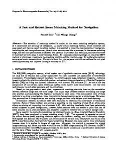
will ”annihilate” each other, despite the fact they represent the same geometric constraints and are therefore not mutually contradictory (see Figure 2). The problem of multiple detections is amplified in matching by view synthesis since covariantly detected local features are often repeatedly discovered in multiple synthetic views. To address this problem, we propose a modified matching strategy denoted first to first geometrically inconsistent – FGINN . Instead of comparing the first to the second closest descriptor distance, the distance of the first descriptor and the closest descriptor that is geometrically inconsistent with the first one is used. We call descriptors in one image geometrically inconsistent if the Euclidean distance between centers of the regions is ≥ n pixels (default: n = 10). The difference of the first-to-second closest ratio strategy and the FGINN strategy is illustrated in Figure 2. 3.4. Geometric verification The last step of the MODS is the geometric verification. It consists of three substeps. 3.4.1. Duplicate filtering The redetection of covariant features in synthetic views results in duplicates in tentative correspondences. The duplicate filtering prunes correspondences with close spatial distance (≈ 5 pixels) of local features in both images – all these correspondences except one – with smallest descriptor distance ratio – are

7

Figure 2: Green regions – correct correspondences rejected by the standard first to second closest ratio test (second closest region is in red), but recovered by the first to first geometrically inconsistent ratio (first geometrically inconsistent region is in yellow) matching strategy. DoG regions (top), MSERs (bottom).

eliminated from the final correspondences list. The number of pruned correspondences can be used later for evaluating the quality (probability of being correct) in PROSAC-like [31] geometric verification. 3.4.2. RANSAC The LO-RANSAC [32] algorithm searches for the maximal set of geometrically consistent tentative correspondences. The model of the transformation is set either to homography or epipolar geometry, or automatically determined by a DegenSAC [26] procedure. 3.4.3. Local affine frame check Since the epipolar geometry constraint is much less restrictive than a homography, wrong correspondences consistent with some (random) fundamental matrix appear. The local affine frame consistency check (LAF-check) eliminates virtually all incorrect correspondences. The procedure uses coordinates of the closest and furthest ellipse points from the ellipse center of both matched local affine frames to check whether the whole local feature is consistent with estimated geometry model (see Figure 3). The check is performed for the geometric 8

] Figure 3: The LAF-check. While centers of both regions A and B are consistent with found homography, farthest (1) and closest (2) points of the ellipse pass the check only for region A.

model obtained by RANSAC. Regions which do not pass the check are discarded from the list of inliers. If the number of correspondences after the LAF-check is fewer than the user defined minimum, matcher continues with the next step of view synthesis. 4. Implementation and parameter setup In this subsection, we discuss the tilt-rotation-detector setups of the MODS algorithm, and threshold selection for the first to first geometrically inconsistent – FGINN matching strategy validation. 4.1. View synthesis for different detectors and descriptors The two main parameters of the view synthesis, tilt {t} sampling and the latitude step ∆φbase , were explored in the following synthetic experiment. A set of simulated views with latitudes angles θ = (0, 20, 40, 60, 65, 70, 75, 80, 85◦ ), corresponding to tilt series t = (1.00, 1.06, 1.30, 2.00, 2.36, 2.92, 3.86, 5.75, 11.47)2 was generated for each of 150 random images from the Oxford Building Dataset3 [33]. Example images are shown in Figure 4. The ground truth affine matrix A was computed for each simulated view using equation (1) and used in the final verification step. The original image was matched against its warped version, and the running time and number of inliers for each combination of the detector, tilt and rotation (see Table 3) were computed. In all, 84 setups for each of the 8 detectors on the 150 image pairs were evaluated. As an example, we show the relation between the density of the view-sphere sampling and the number of images matched for the DoG detector in Figure 5. Since our goal is to find a variety of detector-tilt-rotation configurations operating with different matching ability – run-time trade-offs, we defined “easy”, 2 assuming 3 available

that the original image is the fronto-parallel view at http://www.robots.ox.ac.uk/∼vgg/data/oxbuildings/

9

Figure 4: Two examples of image sets from the synthetic dataset. Original unwarped images are from the Oxford buildings dataset [33].

1 Matched images [%]

Matched images [%]

1

0.5

0

0.8 0.6 0.4 0.2 0 2

2 4 6 8 10 Viewpoint tilt difference

a

b

c

d

e

f

g

i

h

k

j

l

4

72 90

6

120

8

180

10

240 360

Viewpoint tilt difference

Synth tilt setup

3

In−plane synth rotation step [deg]

5 4.5

2.5 4 3.5 3 Time [s]

Time [s]

2

1.5

2.5 2

1 1.5 1

0.5

0.5

0

a

b

c

d

e f g Synth tilt setup

h

i

j

k

l

0 360

240

180 120 In−plane synth, rotation step [deg]

90

72

Figure 5: Top: the percentage of images matched depending the synthetic viewpoint difference for the DoG detector with tilt configurations given in Table 3. Left: different tilt synthesis configurations (for ∆φ = 240◦ ), right: different rotation synthesis configurations (for tilt set (d) = {1,5,9}). Bottom: running time per image pair for the respective configuration.

10

Table 3: View synthesis configuration evaluation. Configuration is a triplet - the detector, descriptor and the set of the synthesized views. DoG-SIFT, Hessian-Affine-SIFT, Harris-Affine-SIFT, Detector-descriptor combination MSER-SIFT, SURF-SURF, SURF-FREAK, AGAST-FREAK, ORB a = {1}, b = {1,2}, c = {1,8}, d = {1,5,9}, e = {1,4},f = {1,4,8}, g = {1,2,4,8}, h √ = {1,3,6,9}, √ i= Tilt set {1,4,8,10}, j = {1,2,4,6,8}, k = {1, 2, 2, 2 2, 4, √ 4 2, 8}, l = {1,2,3,4,5,6,7,8,9}. 360, 240, 180, 120, 90, 72, 60 φbase [◦ ]

“medium” and “hard” problems on the synthetic dataset. Successful two-view matching was defined as recovering n ≥ 50 ground truth correspondences on a synthetically warped image. The threshold is set high – synthetic warping of an image is underestimating the reduction of the number of matchable features induced by the effects of a corresponding viewpoint change e.g. due to nonplanarity of the scene or illumination changes. The matcher is considered to solve an “easy” problem if percentage of the matched images f ≥ 50% of total images, “medium” if f ≥ 90% of images matched and solved “hard” if f ≥ 99% of the images are matched. The experiment with the synthetically warped dataset gives a hint about the limits of configurations. Three configurations that solved the maximum tilt difference for each case fastest for a given detector were selected for evaluation. The configurations are specified in Table 4. The average time necessary to match a given synthetic tilt difference for different detectors with the optimal configuration is shown in Figure 6. The computations were performed on the Intel i7 3.9GHz (8 cores) desktop with 8Gb RAM with parallel processing. Note that view synthesis significantly increases the matching performance of all detectors, but not uniformly. The left plot of Figure 6 shows that a very sparse viewsphere sampling greatly improves matching at almost no computational cost for all detectors. However, after reaching a certain density, additional views do not add correspondences in the hardest cases – see the right graph of Figure 6. The ORB detector-descriptor clearly outperforms other detectors in terms of speed, but fails to match all images with the maximum tilt difference. The Hessian-Affine shown the best performance and it matched all pairs. 4.2. First geometrically inconsistent nearest neighbor ratio correspondence selection strategy The following protocol was used to find the thresholds and to evaluate the performance of the proposed First Geometrically Inconsistent Nearest Neighbor FGINN strategy. First, similarity covariant regions were detected using the DoG detector (we also tried Hessian-Affine, MSER and SURF, with very similar results) and described using four popular descriptors – RootSIFT, SURF, LIOP [35] and MROGH [20] which are typically matched with the secondnearest region SNN strategy. Then for each keypoint descriptor, the first, second

11

6 4

DoG HarrisAffine HessianAffine MSER AGAST−FREAK ORB SURF−FREAK SURF−SURF

2 0

10

10

8

8

6

6

Time [s]

Time [s]

8

Time [s]

10

4 2

2

4 6 8 10 Max synthetic tilt matched

12

0

4 2

2


12

0

2


12

Figure 6: Performance of view synthesis configurations on the synthetic dataset. Average time needed to match (left)“easy”, (center) “medium” and (right)“hard” problems. The time for the fastest detector configuration that solved corresponding problems for a given tilt is shown.

and first geometrically inconsistent descriptors in the other image were found. The matching keypoints were then labeled as correct if their Sampson error was within 1 pixel of the ground truth location given by homography for the image pair, and incorrect otherwise. The experiment was performed on 26 image pairs of the publicly available datasets [9],[34] (image pairs 1-3, precise homography provided) and [36] (the homography was estimated using provided precise ground truth correspondences). The recall-precision curves for correspondences from all images were plot with a varying ratio threshold from 0 to 1 in Figure 7. The FGINN curves for SIFT and SURF slightly outperform standard SNNs, while for LIOP and MROGH the difference is much more significant. The significantly higher benefit of the FGINN rule for LIOP and MROGH can be explained by their lower sensitivity to keypoint shift which in turn means that undesirable suppression of keypoints happens in a larger neighborhood. The lower sensitivity to shifts was experimentally verified. 5. Experiments We have tested MODS and, as a baseline, ASIFT4 and single detector configurations specified in Table 4 on seven public. datasets [10],[30],[37], [38], [39], [40], [41]. Implementation details of the MODS algorithm and parameter setting. The kdtree algorithm from FLANN library [42] was used to efficiently find the N-closest descriptors. The distance ratio thresholds of the FGINN matching strategy were experimentally selected based on the CDFs of matching and non-matching descriptors. The MODS algorithm allows to set the minimum desired number of inliers which have a very low probability to be a random result as a stopping criterion. 4 Reference

code from http://demo.ipol.im/demo/my affine sift

12

Table 4: View synthesis configurations with best synthetic dataset performance. Configurations Detector Easy Medium Hard {t} = {t} = {1; 5; 9}, {t} = {1; 2; 4; 6; 8}, {1; 2; 3; 4; 5; 6; 7; 8; 9}, DoG-SIFT ∆φ = 360◦ /t ∆φ = 60◦ /t ∆φ = 180◦ /t {t} = {t} = {t} = {1; 3; 6; 9}, {1; 2; 3; 4; 5; 6; 7; 8; 9}, {1; 2; 3; 4; 5; 6; 7; 8; 9}, HarrAff-SIFT ∆φ = 360◦ /t ∆φ = 360◦ /t ∆φ = 120◦ /t {t} = {1; 5; 9}, {t} = {1; 5; 9}, {t} = {1; 2; 4; 6; 8}, HessAff-SIFT ∆φ = 360◦ /t ∆φ = 360◦ /t ∆φ = 60◦ /t {t} √ = √ {t} = {1; 8}, {t} = {1; 3; 6; 9}, {1; MSER-SIFT √ 2; 2; 2 2; 4; ◦ ∆φ = 360◦ /t ∆φ = 60◦ /t 4 2; 8}, ∆φ = 60 /t {t} = {1; 4; 8; 10}, {t} = {1; 3; 6; 9}, {t} = {1; 3; 6; 9}, AGAST-FREAK ∆φ = 360◦ /t ∆φ = 60◦ /t ∆φ = 72◦ /t {t} = {t} √ = √ {t} = {1; 5; 9}, {1; 2; 3; 4; 5; 6; 7; 8; 9}, {1; 2; 2; 2 2; 4; ORB ◦ √ ∆φ = 360 /t ◦ ∆φ = 90 /t 4 2; 8}, ∆φ = 72◦ /t {t} √ = {t} = {t} √ = √ √ √ √ {1; {1; {1; SURF-FREAK √ 2; 2; 2 2; 4; ◦ √ 2; 2; 2 2; 4; ◦ √ 2; 2; 2 2; 4; ◦ 4 2; 8}, ∆φ = 60 /t 4 2; 8}, ∆φ = 90 /t 4 2; 8}, ∆φ = 72 /t {t} = {t} = {t} = {1; 5; 9}, {1; 2; 3; 4; 5; 6; 7; 8; 9}, {1; 2; 3; 4; 5; 6; 7; 8; 9}, SURF-SURF ◦ ∆φ = 360 /t ∆φ = 360◦ /t ∆φ = 72◦ /t

The recommended value – 15 inliers to the homography – did not produce a false positive results in experiments. Computations were performed on Intel i3 CPU @ 2.6GHz with 4Gb RAM with 4 cores. 5.1. MODS variants testing on Extreme Viewpoint and Oxford Dataset To evaluate the performance of matching algorithms, we introduce a twoview matching evaluation dataset5 with extreme viewpoint changes, see Table 5. The dataset includes image pairs from publicly available datasets: adam and mag [16], graf [9] and there [34]. The ground truth homography matrices were estimated by LO-RANSAC using√correspondences √ √ from all detectors in view synthesis configuration {t} = {1; 2; 2; 2 2; 4; 4 2; 8}, ∆φ = 72◦ /t. The number of inliers for each image pair was ≥ 50 and the homographies were manually inspected. For the image pairs graf and there precise homographies are provided by Cordes et.al. [34]. Transition tilts τ were computed using equation (1) with SVD decomposition of the linearized homography at center of the first image of the pair (see Table 5). Oxford [9] dataset with 42 image pairs (1-2, ..., 1-6) was used for easier wide baseline problems. Experimental protocol. The evaluated algorithms matched image pairs and the output keypoints correspondences were checked with ground truth homogra5 Available

at http://cmp.felk.cvut.cz/wbs/index.html

13

1

1

0.8

0.8

Precision

Precision

0.6 DoG−SIFT SNN DoG−SIFT FGINN SURF: SNN SURF FGINN DoG−LIOP SNN DoG−LIOP FGINN DoG−MROGH SNN DoG−MROGH FGINN

0.4

0.2

0 0

0.2

0.4

0.6

0.4

0.2

0.6

0.8

1

DoG−SIFT SNN DoG−SIFT FGINN SURF: SNN SURF FGINN DoG−LIOP SNN DoG−LIOP FGINN DoG−MROGH SNN DoG−MROGH FGINN

0 0

0.2

0.4

Recall

0.6

0.8

1

Recall

Figure 7: Comparison of the FGINN and SNN matching strategies for SIFT, SURF, LIOP and MROGH on images from the Oxford [9] and Cordes et.al. [34] datasets. Markers show operationg points for the common distance ratio threshold = 0.8. Matching without (left) view synthesis an using view synthesis (right) with parameters {t} = {1; 5; 9}, ∆φ = 360◦ /t. The recall and precision of the correspondence filtering step, therefore the maximum recall is 1 when all correspondences are kept.

phies. The image pair is considered as solved, when at least 10 output correspondences are correct. Figure 8 compares the different view synthesis configurations. Note that no single detector solved all image pairs. The Hessian-Affine, MSER, Harris-Affine and DoG successfully solved resp. 13, 13, 12 and 13 out of the 15 image pairs however, at the expense of the high computational cost. We also noticed that if one would know the suitable detector and configuration for each image, it is possible to match all image pairs. 15

Pairs matched

10

Best for each pair AGAST_FREAK DoG HarrisAffine HessianAffine MSER ORB SURF_FREAK SURF_SURF

5

0 0

5

10 15 Total time [s]

20

25

15

15

10

10

5

5

0 0

50


200

250

0 0

50

100

150 Total time [s]

200

250

300

Figure 8: Performance of different configurations on the Extreme View Dataset. Cumulative percentage of image pairs successfully matched in a given time for configurations defined in Table 4. Each mark represents one image pair. The fastest detector configuration which was able to match each pair was selected. Left – ’easy’, middle – ’medium’, left – ’hard’ configurations. An images is considered matched if 10 correct inliers were found.

The MODS algorithm with more time-consuming configurations solves all image pairs and does it faster than a suitable configuration for each image pair – see Figure 9. We have tested several variants of the MODS configurations,

14

Table 5: The Extreme View Dataset – EVD. Image sources: C – [34], Ox – [9], M – [16]. # 1 2 Name there graf C Ox Ref. τ – 6.3 3.6 tilt Size 1536 800 x x [pxl] 1024 640 Image 1

#

3 4 adam mag M M 4.8

20

600 600 x x 450 450 Image 2

5 6 7 8 9 10 11 12 13 14 15 grandpkk face girl shop dum index cafe fox cat vin EVD EVD EVD EVD EVD EVD EVD EVD EVD EVD EVD 2.9

7.1

6.9

8.0

9.1

6.9

6

11

2

7

12

3

8

13

4

9

14

5

10

15

Pairs matched

1

1

1

0.8

0.8

11.9

22.5

47

49.8

1000 1000 1000 x x x 563 598 715 Image 2

0.6

0.6 Best single MODS:1−7 MODS:2−7 MODS:3*−6 MODS:3−7 MODS:3,1:7 MODS:2,4,7 MODS:5,1−7 ASIFT

0.4

0.2

0 0

8.5

1000 1000 1000 1000 1000 1000 1000 800 x x x x x x x x 667 750 750 750 562 729 750 533 Image 1 Image 2 Image 1 # #

20


80

100

Best single MODS:1−7 MODS:2−7 MODS:3*−6 MODS:3−7 MODS:3,1:7 MODS:2,4,7 MODS:5,1−7 ASIFT

0.4

0.2

0 0

10

20


50

60

Figure 9: Performance of MODS configurations specified in Table 2. Cumulative percentage of image pairs successfully matched in time. Left - EVD dataset, right - Oxford dataset. The graphs are cropped. Each mark represents one image pair. The fastest single detector configuration which is able to match each pair was selected and plotted separately. Image considered matched if 10 correct inliers was found.

15

Detector DoG

Table 6: ASIFT view synthesis configuration View synthesis setup √ √ √ {S} = {1}, {t} = {1; 2; 2; 2 2; 4; 4 2; 8}, ∆φ = 72◦ /t

stated in Table 2. Experiments shows that the proposed MODS configuration is very fast on the easy WBS problems as in Oxford dataset (see Figure 9, right graph) and has very little overhead on the harder EVD dataset – it is the second best after configuration without ORB steps. The results of the MODS medium configuration – without first sparse synthesis step – shows fruitfulness of the progressive view synthesis. ASIFT is able to match only 6 image pairs from the dataset. The ASIFT algorithm generates a lower number of correct inliers and works slower than our identical DoG configuration (which has the same tilt-rotation set). The main causes are the elimination of ”one-to-many”, including correct, correspondences, the inferiority of the standard second closest ratio matching strategy and a simple brute-force algorithm of matching used in ASIFT. Fig. 10 shows the breakdown of the computational time. The most time consuming parts – detection and description (including the dominant orientation estimation) – take 40% and 35% resp. of the all time. Without applying the fast SIFT computation from [29], the SIFT description takes more than 50% of the time. The ORB is an exception - the synthesis is not so profitable, since it takes more time than detection and description itself. Note that the whole process is almost linear in the area of the synthesized views. The only super-linear part, matching, takes only 10% of the time.

MODS

Synthesis Detection Orientation Description Matching RANSAC Misc

SURF DoG ORB MSER HA 0

20

40 60 Time [%]

80

100

Figure 10: Percentages of time spent in the main stages of the matching with view synthesis process on a single core, easy configuration. Detection and SIFT description, i.e. the dominant gradient estimation and the descriptor computation are the most time-consuming parts.

16

5.2. MODS testing on a non-planar dataset 5.2.1. The dataset and evaluation protocol The evaluation dataset consists of 35 image sequences taken from the Turntable dataset [10] (“Bottom” camera) shown in Table 7. Eight image sets contain objects with relatively large planar surfaces and the remaining ones are lowtextured, “general 3D” objects. The view marked as “0◦ ” in the Turntable dataset was used as a reference view and 0−90◦ and 270-355 ◦ views with a 5◦ step were matched against it using the procedure described in Sec. 5, forming a [−90◦ , 90◦ ] sequence. Note that the reference view is not usually the “frontal” or “side” view, but rather some intermediate view which caused asymmetry in results (see Fig. 11, Table 8). The output of the matchers is a set of the correspondences and the estimated geometrical transformation. The accuracy of the matched correspondences was chosen as the performance criterion, similarly to the protocol in [43]. For all output correspondences, the symmetrical epipolar error [27] eSymEG was computed according to the following expression: 2 1 1 + , (2) eSymEG (F, u, v) = v> Fu × (Fu)21 + (Fu)22 (F> v)21 + (F> v)22 where F – fundamental matrix, u, v – corresponding points, (Fu)2j – the square of the j-th entry of the vector Fu. The ground truth fundamental matrix was obtained from the difference in camera positions [27], assuming that turntable is fixed and the camera moved around the object, according to the following equation: F = K −> RK > [KR> t]× ,    cos φ 0 − sin φ ,K =  1 0 R= 0 sin φ 0 cos φ

mf FRX

0 0

0 nf FRY

0

m 2 n 2





 sin φ ,t = r , 0 1 − cos φ 1 (3)

where R is the orientation matrix of the second camera, K – the camera projection matrix, t – the virtual translation of the second camera, r – the distance from camera to the object, φ – the viewpoint angle difference, FRX , FRY – the focal plane resolution, f – the focal length, m, n – the sensor matrix width and height in pixels. The last five parameters were obtained from EXIF data. One of the evaluation problems is that background regions, i.e. regions that are not on the object placed on the turntable, are often detected and matched influencing the geometry transformation estimation. The matches are correct, but consistent with an identity transform of the (background of) the test images, not the fundamental matrix associated with the movement of the object on the turntable. In order to solve this problem, the median value of the correspondence errors was chosen as the measure of precision because of its tolerance to the low number of outliers (e.g. the above-mentioned background correspondences), and

17

Table 7: Reference views of the image sequences used in the evaluation (from [10]).

Abroller

Bannanas

Camera2

Car

Car2

CementBase

Cloth

Conch

Desk

Dinosaur

Dog

DVD

FloppyBox

FlowerLamp

Gelsole

GrandfatherClock

Horse

Keyboard

Motorcycle

MouthGuard

PaperBin

PS2

Razor

RiceCooker

Rock

RollerBlade

Spoons

TeddyBear

Toothpaste

Tricycle

Tripod

VolleyBall

18

Table 8: Experiment on the 3D dataset. The configurations are defined in Table 4. The number of correctly matched image pairs and the run-time per pair. Best results are boxed . Results within 90% of the best are in bold. The configurations are sorted by average time for image pair. Image sets solved (out of 35) Viewpoint angular difference Time Matcher 0◦ 5◦ 10◦ 15◦ 20◦ 25◦ 30◦ 35◦ 40◦ ≥ 45◦ [s] HessianAffine easy 35 32 29 26 22 17 13 14 9 6 0.9 SURF-SURF easy 35 31 24 18 15 12 7 5 4 2 0.9 HessianAffine medium 35 30 26 24 18 17 12 10 7 10 1.0 ORB easy 35 31 27 20 16 11 10 5 5 4 1.0 AGAST-FREAK easy 35 28 29 26 19 17 12 9 7 6 1.3 DoG easy 35 33 30 22 18 12 10 7 5 3 1.4 MSER easy 35 28 22 21 15 13 10 8 7 5 1.5 SURF-SURF hard 35 26 16 11 9 7 6 4 3 3 2.1 HarrisAffine easy 35 29 22 12 8 6 5 3 2 1 2.7 AGAST-FREAK hard 35 31 28 25 20 17 15 10 8 5 4.7 HarrisAffine medium 35 27 20 11 7 6 5 4 3 2 4.7 HessianAffine hard 35 29 24 20 20 17 15 11 9 6 5.6 DoG medium 35 32 26 21 16 11 10 9 6 5 6.8 AGAST-FREAK medium 35 29 23 22 18 14 13 6 6 6 7.2 ORB hard 35 31 24 19 16 7 5 4 1 4 7.3 SURF-FREAK easy 35 25 21 13 10 8 6 3 2 2 7.3 ORB medium 35 30 26 18 17 10 5 4 2 4 8.3 SURF-FREAK medium 35 22 15 10 9 7 6 4 1 2 9.1 SURF-SURF medium 35 25 20 13 11 7 3 3 2 2 10.7 SURF-FREAK hard 35 25 17 14 10 9 4 3 1 2 10.9 MSER hard 35 29 24 24 19 16 12 13 8 8 14.5 HarrisAffine hard 35 27 16 8 5 5 5 3 2 2 15.2 DoG hard 35 32 24 17 16 13 12 8 7 8 16.7 MSER medium 35 29 26 23 21 14 10 9 7 9 17.5 ASIFT 35 32 24 18 13 8 7 5 4 3 27.6 MODS:1-7 35 31 27 27 22 22 14 9 10 11 6.7

its sensitivity to the incorrect geometric model estimated by RANSAC. An image pair is considered as correctly matched if the median symmetrical epipolar error on the correspondences using ground truth fundamental matrix is ≤ 6 pixels. 5.2.2. Results Figure 11 and Table 8 show the percentage and the number of image sequences respectively for which the reference and tested views for the given viewing angle difference were matched correctly. The difference between easy, medium and hard configurations is small for structured scenes — unlike planar ones. Difficulties in matching are caused not by the inability to detect distorted regions but by object self-occlusions. Therefore synthesis of the additional views does not bring more correspondences. Experiments with view synthesis confirmed [10] results that the HessianAffine outperforms other detectors for matching of structured scenes and can

19

easy−AGAST−FREAK −15° 0° 15° 30°

medium−AGAST−FREAK −15° 0° 15° 30°

−30° −45°

45°

−60°

−45° 60°

−75°

75°

−90°

90°

45°

−60°

60°

−75°

75°

−90°

90°

easy−DoG −15° 0° 15° −30°

30°

−30° 45°

−60° −75°

75°

−90°

90°

60°

−75°

75°

−90°

90°

easy−HarrisAffine −15° 0° 15° 30°

−45°

45°

−60°

−45° 60°

−75°

75°

−90°

90°

75°

−90°

90°

30° 45°

−60°

−45° 60°

−75°

75°

−90°

90°

75°

−90°

90°

30°

−45°

−30° 45°

−60° −75°

75°

−90°

90°

75°

−90°

90°

easy−ORB −15° 0° 15° −30°

30°

−45°

−30° 45°

−60° −75°

75°

−90°

90°

75°

−90°

90°

easy−SURF−FREAK −15° 0° 15° −30° 30° −45°

45°

−60°

−45° 60°

−75°

75°

−90°

90°

75°

−90°

90°

easy−SURF−SURF −15° 0° 15° −30° −45°

45°

−60°

−45° 60°

−75°

75°

−90°

90°

75°

−90°

90°

−30° −45°

−75° −90°

90°

−60°

45° 60° 75° 90°

−60° −75° −90°

0

1

60°

−75°

0.5

75°

−90°

90°

−60°

0

1

60°

−75°

0.5

75°

−90°

90°

ASIFT −15° 0° 15° −30° 30° −45° 45°

30°

0.5

75°

hard−SURF−SURF −15° 0° 15° −30° 30° −45° 45° 60°

−75°

0

1

60°

−90°

45°

−60°

MODS −15° 0° 15°

−60°

−60°

medium−SURF−SURF −15° 0° 15° −30° 30°

30°

90°

hard−SURF−FREAK −15° 0° 15° −30° 30° −45° 45° 60°

−75°

0.5

75°

−75°

45°

−60°

60°

−90°

medium−SURF−FREAK −15° 0° 15° −30° 30°

0

1

hard−ORB −15° 0° 15° −30° 30° −45° 45° 60°

−75°

90°

−60°

45°

−60°

0.5

75°

−75°

30°

−45° 60°

60°

−90°

medium−ORB −15° 0° 15°

0

1

hard−MSER −15° 0° 15° −30° 30° −45° 45° 60°

−75°

90°

−60°

45°

−60°

0.5

75°

−75°

30°

−45° 60°

60°

−90°

medium−MSER −15° 0° 15°

0

1

hard−HessianAffine −15° 0° 15° −30° 30° −45° 45° 60°

−75°

easy−MSER −15° 0° 15° −30°

−60°

45°

−60°

90°

−75°

medium−HessianAffine −15° 0° 15° −30° 30°

0.5

75°

hard−HarrisAffine −15° 0° 15° −30° 30° −45° 45° 60°

−75°

easy−HessianAffine −15° 0° 15° −45°

−75°

0

1

60°

−90°

45°

−60°

90°

−60°

medium−HarrisAffine −15° 0° 15° −30° 30°

0.5

75°

hard−DoG −15° 0° 15° −30° 30° −45° 45°

45°

−60°

1

60°

−90°

30°

−45° 60°

−30°

−60° −75°

medium−DoG −15° 0° 15°

−45°

−30°

hard−AGAST−FREAK −15° 0° 15° −30° 30° −45° 45°

−30°

0

1

60°

0.5

75° 90°

0

Figure 11: A comparison of view synthesis configurations on the Turntable dataset [10]. The 20 fraction of correctly matched images for a given viewpoint difference.

Figure 12: Correspondences found by MODS. Green – corresponding regions, cyan – epipolar lines. Objects with significant self-occlusion and mostly homogenious texture were selected.

21

Figure 13: Examples from the Extreme Zoom Dataset

be used alone in such scenes. MODS shows similar performance, but is slower than the Hessian-Affine configuration. The computations were performed on Intel i5 3.0GHz (4 cores) desktop with 16Gb RAM. Examples of the matched images are shown in Fig. 12. 5.3. MODS testing on other datasets 5.3.1. Extreme zoom dataset We introduce the Extreme Zoom dataset (EZD), which is a small subset of the retrieval dataset used in [41]. It consists of six sets of images with an increasing level of zoom (see examples in Figure 13). The state-of-the art matcher – ASIFT [16] and registration algorithm DualBootstrap [44] as well a results for MSER, ORB and Hessian-Affine matchers without view synthesis were compared to MODS. Image pairs are matched with tested algorithms. An image pair is considered solved when at least 10 output correspondences are correct. Results are shown in Table 9. Table 9: Results on the Extreme Zoom Dataset. Matcher Zoom level, matched I (max 6) II (max 6) III (max 6) IV (max 4) ORB 0 0 0 0 MSER 2 2 1 0 DBstrap 3 1 0 0 HessAff 5 3 2 0 ASIFT 3 3 2 0 MODS 6 3 3 0

5.3.2. Ultra wide-baseline dataset The MODS performance was evaluated on the city-from-air dataset from [37]. The dataset comprises 30 pairs (examples shown in Figure 14) of photographs of buildings taken from the air. The view points difference is quite large, the images contain repeated structures, illumination differs. The authors proposed a matcher based on HoG [45] descriptor with view synthesis and compare it to ASIFT and D-Nets [46] for skyscraper frontal face matching. We 22

follow the evaluation protocol which considers a pair matched correct only if the facade plane is matched (≥ 75% correct inliers). If the output homography was ground/roof, it is considered incorrect. The results are shown in Table 10. Note that no special adjustment is done in MODS for homography selection, so the reported performance is a lower bound.

Figure 14: Examples of image pairs from the Ultra wide-baseline dataset [37]

Table 10: Results on Ultra wide-baseline dataset (all results except Method Correct (or shifted) Different plane Altwaijry and Belongie [37] 9 1 ASIFT-homography 1 5 D-Nets 7 2 MODS 8 1

MODS taken from [37]) Failure/ground plane 20 24 21 21

5.3.3. Datasets with other than geometric changes Despite being designed for (extreme) wide baseline stereo problems, MODS performance was evaluated on other datasets: GDB-ICP [39] (modality, viewpoint and photometry changes), SymBench [38] (photometrical changes and photo-vs-painting pairs), and MMS [40] (infrared-vs-visible pairs) – see Table 11. The state-of-the art matcher – ASIFT [16] and registration algorithm DualBootstrap [44] as well a results for MSER, ORB and Hessian-Affine matchers without view synthesis were compared to MODS.

Short name GDB-ICP SymBench MMS EVD

Table 11: Evaluation Proposed by Kelman et.al. [39], 2007 Hauagge and Snavely [38], 2012 Aguilera et.al. [40], 2012 Mishkin et.al. [30], 2013

Datasets #images 22 pairs 46 pairs 100 pairs 15 pairs

Nuisance Illumination, modality Illumination, modality Modality Viewpoint change

Image pairs are matched with the tested algorithms. Output keypoints correspondences were checked against the ground truth homographies. An image pair is considered solved when at least 10 output correspondences are correct Our primary evaluation criterion is the ability to find sufficiently correct geometric transformations in a reasonable time; accurate geometry can be found in consecutive step. 23

The computations were performed on Intel i3 3.0GHz desktop (4 cores) with 4Gb RAM. Results are shown in the Table 12. MODS is the fastest method and it is able to match the most image pairs in GDB-ICP and SymBench datasets without using symmetrical parts or other problem-specific features. Images from the MMS dataset (as well as other thermal images) produce a small number of features as they do not contain many textured surfaces, and have very short geometrical baseline. Those are the main reasons why area-based method – Dual-Bootstrap – work significantly better than the feature-based methods. After lowering the threshold for detectors allowing to detect more feature points and using the orientation restricted SIFT [47] in addition to the RootSIFT, MODS-IR solved 83 out of 100 image pairs from MMS dataset. Table 12: Performance on non-WBS datasets. For comparison, results of MSER, ORB and Hessian-Affine matchers without view synthesis are added. Best results are in bold, average time per image pair is shown. Matcher GDB-ICP SymBench MMS EVD pairs time pairs time pairs time pairs time solved [s] solved [s] solved [s] solved [s] ASIFT 15/22 41.5 27/46 14.7 8/100 3.2 5/15 12.4 MODS:1-7 17/22 2.8 38/46 3.7 12/100 2.0 15/15 2.4 DBstrap 16/22 17.6 38/46 21.7 79/100 9.3 0/15 1.9 ORB 0/22 0.2 0/46 0.4 0/100 0.1 0/15 0.3 MSER 8/22 1.7 21/46 0.8 0/100 0.2 4/15 0.6 HessAff 11/22 1.9 29/46 1.5 2/100 0.4 2/15 1.1 MODS-IR:1-7 21/22 7.6 39/46 15.1 83/100 9.1 14/15 8.6

6. Conclusions An algorithm for two-view matching called Matching On Demand with view Synthesis algorithm (MODS) was introduced. The most important contributions of the algorithm are its ability to adjust its complexity to the problem at hand, and its robustness, i.e. the ability to solve a broader range of widebaseline problems than the state of the art. This is achieved while being fast on simple problems. The apparent robustness vs. speed trade-off is finessed by the use of progressively more time-consuming feature detectors, and by on-demand generation of synthesized images that is performed until a reliable estimate of geometry is obtained. The MODS method demonstrates that the answer to the question ”which detector is the best?” depends on the problem at hand, and that it is fruitful to focus on the ”how to combine detectors” problem. We are the first to propose view synthesis for two-view wide-baseline matching with affine-covariant detectors, which is superficially counter-intuitive, and we show that matching with the Hessian-Affine or MSER detectors outperforms the state-of-the-art ASIFT. View synthesis performs well when used with simple and very fast detectors like ORB, which obtains results similar to ASIFT but in orders of magnitude shorter time. 24

Minor contributions include an improved method for tentative correspondence selection, applicable both with and without view synthesis and a modification of the standard first to second nearest distance rule increases the number of correct matches by 5-20% at no additional computational cost. The evaluation of the MODS algorithm was carried out both on standard publicly available datasets as well as a new set of geometrically challenging wide baseline problems that we collected and will make public. The experiments show that the MODS algorithm solves matching problems beyond the state-of-theart and yet is comparable in speed to standard wide-baseline matchers on easy problems. Moreover, MODS performs well on other classes of difficult two-view problems like matching of images from different modalities, with large difference of acquisition times or with significant lighting changes. Acknowledgements The authors were supported by The Czech Science Foundation Project GACR P103/12/G084. References References [1] P. Pritchett, A. Zisserman, Wide baseline stereo matching, in: Computer Vision, 1998. Sixth International Conference on, 1998, pp. 754–760. doi: 10.1109/ICCV.1998.710802. [2] K. Mikolajczyk, C. Schmid, A performance evaluation of local descriptors, IEEE Transactions on Pattern Analysis and Machine Intelligence 27(10) (2005) 1615–1630. [3] T. Tuytelaars, K. Mikolajczyk, Local Invariant Feature Detectors: A Survey, Now Publishers Inc., Hanover, MA, USA, 2008. [4] J. Matas, O. Chum, M. Urban, T. Pajdla, Robust wide baseline stereo from maximally stable extrema regions, in: In British Machine Vision Conference, 2002, pp. 384–393. [5] K. Mikolajczyk, C. Schmid, Scale & affine invariant interest point detectors, Int. J. Comput. Vision 60 (1) (2004) 63–86. [6] D. G. Lowe, Distinctive image features from scale-invariant keypoints, Int. J. Comput. Vision 60 (2) (2004) 91–110. doi:10.1023/B:VISI. 0000029664.99615.94. URL http://dx.doi.org/10.1023/B:VISI.0000029664.99615.94 [7] H. Bay, T. Tuytelaars, L. V. Gool, Surf: Speeded up robust features, in: In ECCV, 2006, pp. 404–417.

25

[8] S. Belongie, J. Malik, J. Puzicha, Shape matching and object recognition using shape contexts, Pattern Analysis and Machine Intelligence, IEEE Transactions on 24 (4) (2002) 509–522. doi:10.1109/34.993558. [9] K. Mikolajczyk, T. Tuytelaars, C. Schmid, A. Zisserman, J. Matas, F. Schaffalitzky, T. Kadir, L. V. Gool, A comparison of affine region detectors, International Journal of Computer Vision 65 (2005) 2005. [10] P. Moreels, P. Perona, Evaluation of features detectors and descriptors based on 3d objects, International Journal of Computer Vision 73 (3) (2007) 263–284. doi:10.1007/s11263-006-9967-1. URL http://dx.doi.org/10.1007/s11263-006-9967-1 [11] E. Rosten, T. Drummond, Machine learning for high-speed corner detection, in: In European Conference on Computer Vision, 2006, pp. 430–443. [12] E. Mair, G. D. Hager, D. Burschka, M. Suppa, G. Hirzinger, Adaptive and generic corner detection based on the accelerated segment test, in: European Conference on Computer Vision (ECCV’10), 2010. URL http://www6.in.tum.de/Main/ResearchAgast [13] E. Rublee, V. Rabaud, K. Konolige, G. Bradski, Orb: An efficient alternative to sift or surf, in: Computer Vision (ICCV), 2011 IEEE International Conference on, 2011, pp. 2564–2571. doi:10.1109/ICCV.2011.6126544. [14] S. Leutenegger, M. Chli, R. Y. Siegwart, Brisk: Binary robust invariant scalable keypoints, in: Proceedings of the 2011 International Conference on Computer Vision, ICCV ’11, IEEE Computer Society, Washington, DC, USA, 2011, pp. 2548–2555. doi:10.1109/ICCV.2011.6126542. [15] A. Alahi, R. Ortiz, P. Vandergheynst, FREAK: Fast Retina Keypoint, in: IEEE Conference on Computer Vision and Pattern Recognition, IEEE Conference on Computer Vision and Pattern Recognition, Ieee, New York, 2012, cVPR 2012 Open Source Award Winner. [16] J.-M. Morel, G. Yu, Asift: A new framework for fully affine invariant image comparison, SIAM J. Img. Sci. 2 (2) (2009) 438–469. [17] J.-M. M. Guoshen Yu, Asift: An algorithm for fully affine invariant comparison, Image Processing On Line. [18] H. Aanaes, A. Dahl, K. Steenstrup Pedersen, Interesting interest points, International Journal of Computer Vision 97 (2012) 18–35. [19] S. Wang, Z. Zhao, P. Yu, Z. Guang, Infrared/visible image matching algorithm based on nsct and daisy, in: Image and Signal Processing (CISP), 2011 4th International Congress on, Vol. 4, 2011, pp. 2072–2075. doi:10.1109/CISP.2011.6100604.

26

[20] B. Fan, F. Wu, Z. Hu, Rotationally invariant descriptors using intensity order pooling, IEEE Transactions on Pattern Analysis and Machine Intelligence 34 (10) (2012) 2031–2045. doi:10.1109/TPAMI.2011.277. [21] V. Lepetit, P. Fua, Keypoint recognition using randomized trees, IEEE Trans. Pattern Anal. Mach. Intell. 28 (9) (2006) 1465–1479. doi:10.1109/ TPAMI.2006.188. URL http://dx.doi.org/10.1109/TPAMI.2006.188 [22] L. Moisan, B. Stival, A probabilistic criterion to detect rigid point matches between two images and estimate the fundamental matrix, Int. J. Comput. Vision 57 (3) (2004) 201–218. doi:10.1023/B:VISI.0000013094.38752. 54. [23] W. Liu, Y. Wang, J. Chen, J. Guo, Y. Lu, A completely affine invariant image-matching method based on perspective projection, Mach. Vision Appl. 23 (2) (2012) 231–242. doi:10.1007/s00138-011-0347-7. URL http://dx.doi.org/10.1007/s00138-011-0347-7 [24] Y. Pang, W. Li, Y. Yuan, J. Pan, Fully affine invariant surf for image matching, Neurocomputing 85 (0) (2012) 6 – 10. doi:10.1016/j.neucom. 2011.12.006. [25] P.-E. Forssén, D. Lowe, Shape descriptors for maximally stable extremal regions, in: IEEE International Conference on Computer Vision, Vol. CFP07198-CDR, IEEE Computer Society, Rio de Janeiro, Brazil, 2007. [26] O. Chum, T. Werner, J. Matas, Two-view geometry estimation unaffected by a dominant plane, in: Proceedings of the 2005 IEEE Computer Society Conference on Computer Vision and Pattern Recognition (CVPR’05) Volume 1 - Volume 01, CVPR ’05, IEEE Computer Society, Washington, DC, USA, 2005, pp. 772–779. doi:10.1109/CVPR.2005.354. URL http://dx.doi.org/10.1109/CVPR.2005.354 [27] R. I. Hartley, A. Zisserman, Multiple View Geometry in Computer Vision, 2nd Edition, Cambridge University Press, ISBN: 0521540518, 2004. URL http://www.robots.ox.ac.uk/~vgg/hzbook/ [28] R. Arandjelović, A. Zisserman, Three things everyone should know to improve object retrieval, in: IEEE Conference on Computer Vision and Pattern Recognition, 2012. [29] K. Lenc, J. Matas, D. Mishkin, A few things one should know about feature extraction, description and matching, in: Z. K´ ukelová, J. Heller (Eds.), CVWW 2014: Proceedings of the Computer Vision Winter Workshop 2014, Czech Society for Cybernetics and Informatics, Prague, Czech Republic, 2014, pp. 67–74.

27

´ [30] D. Mishkin, M. Perdoch, J. Matas, Two-view matching with view synthesis revisited, Research Report CTU–CMP–2013–15, Center for Machine Perception, K13133 FEE Czech Technical University, Prague, Czech Republic (June 2013). [31] O. Chum, J. Matas, Matching with prosac ” progressive sample consensus, in: Proceedings of the 2005 IEEE Computer Society Conference on Computer Vision and Pattern Recognition (CVPR’05) - Volume 1 - Volume 01, CVPR ’05, IEEE Computer Society, Washington, DC, USA, 2005, pp. 220–226. doi:10.1109/CVPR.2005.221. URL http://dx.doi.org/10.1109/CVPR.2005.221 [32] O. Chum, J. Matas, J. Kittler, Locally Optimized RANSAC, 2003, pp. 236–243. URL http://www.springerlink.com/content/5xx8b4q181pkey4q [33] J. Philbin, O. Chum, M. Isard, J. Sivic, A. Zisserman, Object retrieval with large vocabularies and fast spatial matching, in: Proceedings of the IEEE Conference on Computer Vision and Pattern Recognition, 2007. [34] K. Cordes, B. Rosenhahn, J. Ostermann, Increasing the accuracy of feature evaluation benchmarks using differential evolution, in: IEEE Symposium Series on Computational Intelligence (SSCI) - IEEE Symposium on Differential Evolution (SDE), 2011. URL http://dx.doi.org/10.1109/SDE.2011.5952056 [35] R. Gupta, H. Patil, A. Mittal, Robust order-based methods for feature description, in: Computer Vision and Pattern Recognition (CVPR), 2010 IEEE Conference on, 2010, pp. 334–341. doi:10.1109/CVPR.2010. 5540195. [36] K. Lebeda, J. Matas, O. Chum, Fixing the locally optimized ransac, in: R. Bowden, J. Collomosse, K. Mikolajczyk (Eds.), Proceedings of the British Machine Vision Conference, BMVA, London, UK, 2012, pp. 1013– 1023. doi:http://dx.doi.org/10.5244/C.26.95. [37] H. Altwaijry, S. J. Belongie, Ultra-wide baseline aerial imagery matching in urban environments, in: British Machine Vision Conference, BMVC 2013, Bristol, UK, September 9-13, 2013, 2013. doi:10.5244/C.27.15. URL http://dx.doi.org/10.5244/C.27.15 [38] D. C. Hauagge, N. Snavely, Image matching using local symmetry features, in: CVPR, 2012, pp. 206–213. [39] A. Kelman, M. Sofka, C. V. Stewart, Keypoint descriptors for matching across multiple image modalities and non-linear intensity variations, in: CVPR, 2007.

28

[40] C. Aguilera, F. Barrera, F. Lumbreras, A. D. Sappa, R. Toledo, Multispectral image feature points, Sensors 12 (9) (2012) 12661–12672. doi: 10.3390/s120912661. URL http://www.mdpi.com/1424-8220/12/9/12661 [41] A. Mikulik, F. Radenovic, O. Chum, J. Matas, Efficient image detail mining, in: ACCV, 2014. [42] M. Muja, D. G. Lowe, Fast approximate nearest neighbors with automatic algorithm configuration, in: International Conference on Computer Vision Theory and Application VISSAPP’09), INSTICC Press, 2009, pp. 331–340. [43] A. L. Dahl, H. Aanaes, K. S. Pedersen, Finding the best feature detectordescriptor combination, in: Proceedings of the 2011 International Conference on 3D Imaging, Modeling, Processing, Visualization and Transmission, 3DIMPVT ’11, IEEE Computer Society, Washington, DC, USA, 2011, pp. 318–325. doi:10.1109/3DIMPVT.2011.47. URL http://dx.doi.org/10.1109/3DIMPVT.2011.47 [44] G. Yang, C. Stewart, M. Sofka, C.-L. Tsai, Registration of challenging image pairs: Initialization, estimation, and decision, Pattern Analysis and Machine Intelligence, IEEE Transactions on 29 (11) (2007) 1973–1989. doi: 10.1109/TPAMI.2007.1116. [45] N. Dalal, B. Triggs, Histograms of oriented gradients for human detection, in: Computer Vision and Pattern Recognition, 2005. CVPR 2005. IEEE Computer Society Conference on, Vol. 1, 2005, pp. 886–893vol. 1. doi: 10.1109/CVPR.2005.177. [46] F. von Hundelshausen, D-nets: Beyond patch-based image descriptors, in: Proceedings of the 2012 IEEE Conference on Computer Vision and Pattern Recognition (CVPR), CVPR ’12, IEEE Computer Society, Washington, DC, USA, 2012, pp. 2941–2948. [47] K.-C. Chen, W.-H. Tsai, Vision-based autonomous vehicle guidance for indoor security patrolling by a sift-based vehicle-localization technique, Vehicular Technology, IEEE Transactions on 59 (7) (2010) 3261 –3271. doi:10.1109/TVT.2010.2052079.

29