NPTEL - ADVANCED FOUNDATION ENGINEERING-1. Module 1.
GEOTECHNICAL PROPERTIES OF SOIL AND OF. REINFORCED SOIL (
Lectures 1 to 4).
NPTEL - ADVANCED FOUNDATION ENGINEERING-1
Module 1 GEOTECHNICAL PROPERTIES OF SOIL AND OF REINFORCED SOIL (Lectures 1 to 4)
Topics
1.1 INTRODUCTION 1.2 GRAIN-SIZE DISTRIBUTION Sieve Analysis Hydrometer Analysis
1.3 SIZE LIMITS FOR SOILS 1.4 WEIGHT-VOLUME RELATIONSHIPS 1.5 RELATIVE DENSITY 1.6 ATTERBERG LIMITS 2.1
SOIL CLASSIFICATION SYSTEMS
2.2
AASHTO System Unified System Examples and Solutions
2.3
HYDRAULIC CONDUCTIVITY OF SOIL
2.4
STEADY-STATE SEEPAGE
2.5
FILTER DESIGN CRITERIA
2.6
EFFECTIVE STRESS CONCEPT
NPTEL - ADVANCED FOUNDATION ENGINEERING-1
3.1
CAPILLARY RISE IN SOIL
3.2
CONSOLIDATIONS-GENERAL
3.3
CONSOLIDATION SETTLEMENT CALCULATION
3.4
TIME RATE OF CONSOLIDATION
4.1 SHEAR STRENGTH Direct Shear Test Triaxial Tests 4.2 4.3
UNCONFINED COMPRESSION TES COMMENTS ON SHEAR STRENGTH PARAMETERS
Drained Friction Angle of Granular Soils Drained Friction Angle of Cohesive Soils 4.4 SENSITIVITY 4.5 SOIL REINFORCEMENT-GENERAL 4.6 CONSIDERATIONS FOR SOIL REINFORCEMENT Metal Strips Nonbiodegradable Fabrics Geogrids PROBLEMS REFERENCE
NPTEL - ADVANCED FOUNDATION ENGINEERING-1
Module 1
Lectures 1 GEOTECHNICAL PROPERTIES OF SOIL AND OF REINFORCE SOIL Topics 1.1
INTRODUCTION
1.2
GRAIN-SIZE DISTRIBUTION Sieve Analysis Hydrometer Analysis
1.3 SIZE LIMITS FOR SOILS 1.4 WEIGHT-VOLUME RELATIONSHIPS 1.5 RELATIVE DENSITY 1.6 ATTERBERG LIMITS
1.1 INTRODUCTION The design of foundations of structures such as buildings, bridges, and dams generally requires a knowledge of such factors as (a) the load that will be transmitted by the superstructure to the foundation system, (b) the requirements of the local buildings code, (c) the behavior and stress-related deformability of soils that will support the foundation system, and d the geological conditions of the under consideration. To a foundation engineer, the last two factors are extremely important because they concern soil mechanics. The geotechnical properties of a soil-such as the grain-size distribution, plasticity, compressibility, and shear strength-can are assessed by proper laboratory testing. And, recently, emphasis has been placed on in situ determination of strength and deformation properties of soil, because this process avoids the sample disturbances that occur during field exploration. However, under certain circumstances, all of the needed parameters cannot be determined or are not determined because of economic or other reasons. In such cases, the engineer must make certain assumptions regarding
NPTEL - ADVANCED FOUNDATION ENGINEERING-1 the properties of the soil. The assessment of the accuracy of soil parameters-whether they were determined in the laboratory and the field or were assumed-the engineer must have a good grasp of the basic principles of soil mechanics. At the same time, he or she must realize that the natural soil deposits on which foundation are constructed are not homogeneous is most cases. Thus the engineer must have a thorough understanding of the geology of the are-that is, the origin and nature of soil stratification and also the groundwater conditions. Foundation engineering is a clever combination of soil mechanics, engineering geology, and proper judgment derived from past experience. To a certain extent, it may be called an “art”. When determining which foundation is the most economical, the engineer must consider the superstructure load, the subsoil conditions, and the desired tolerable settlement. In general, foundations of buildings and bridges may be divided into two major categories: (a) shallow foundations and (2) deep foundations. Spread footings, wall footings, and mat foundations are all shallow foundations. In most shallow foundations, the depth of embedment can be equal to or less than three to four the width of the foundation. Pile and drilled shaft foundations are deep foundations. This chapter serves primarily as a review of the basic geotechnical properties of soil. It includes topics such as grain-size distribution, plasticity, and soil classification effective stress, consolidation, and shear strength parameters. It is based on assumption that you have already been exposed to these concepts in a basic mechanics course. 1.2 GRAIN-SIZE DISTRIBUTION In any soil mass, the sizes of various soil grains vary greatly. To classify a properly, you must know its grain-size distribution. The grain-size distribution of coarsegrained soil is generally determined by means of sieve analysis. For a fine grained soil, the grain-size distribution can be obtained by means of hydrometer analysis. The fundamental features of these analyses are presented in this section. For detailed descriptions, see any soil mechanics laboratory manual (for exam, Das, 1997). 1.2.1 Sieve Analysis A sieve analysis is conducted by taking a measured amount of dry, well-pulverized soil and passing it through a stack of progressively finer sieves with a pan at bottom. The amount of soil retained on each sieve is measured, and the cumulative percentage of soil passing through each sieve is determined. This percentage generally referred to as percent finer. Table 1 contains a list of U. S. sieve number and the corresponding size of their hole openings. These sieves are commonly used for the analysis of soil classification purposes. The percent finer for each sieve determined by a sieve analysis is plotted semi logarithmic graph paper, as shown in figure1.1Note that the grain diameter D, is plotted on the logarithmic scale, and the percent finer is plotted on the arithmetic scale.
NPTEL - ADVANCED FOUNDATION ENGINEERING-1
Figure 1.1 Grain-size distribution curve of a coarse grained soil obtained from sieve analysis Two parameters can be determined from the grain-size distribution curves coarsegrained soils: (1) the uniformity coefficient (Cu ) and (2) the coefficient gradation, or coefficient of curvature (Cz ). These coefficients are Table U. S. Standard Sieve Sizes Sieve no. 4 6 8 10 16 20 30 40 50 60 80 100 140 170 200 270 D
Cu = D 60 Cz = D
10
D 230
60 × D 10
Opening (mm) 4.750 3.350 2.360 2.000 1.180 0.850 0.600 0.425 0.300 0.250 0.180 0.150 0.106 0.088 0.075 0.053 [1.1]
[1.2]
NPTEL - ADVANCED FOUNDATION ENGINEERING-1 whereD10 , D30 , and D60 are the diameters corresponding to percents fines the 10, 30, and 60%, respectively. For the grain-size distribution curve shown in figure 1.1,D10 = 0.08 D30 = 0.17 mm, and D60 = 0.57 mm. Thus the values of Cu and Cz are Cu =
Cz =
0.57 = 7.13 0.08
0.172 = 0.63 (0.57)(0.08)
Parameters Cu and Cz are used in the Unified Soil Classification System, which described later in this chapter. Hydrometer Analysis Hydrometer analysis is based on the principle of sedimentation of soil particles water. This test involves the use of 50 grams of dry, pulverized soil. A deflocculating agent is always added to the soil. The most common deflocculating agent used the hydrometer is 125 cc of 4% solution of sodium hexametaphosphate. The soil is allowed to soak for at least 16 hours in the deflocculating agent. After the soaking period, distilled water is added, and the soil-deflocculating agent mixture is thoroughly agitated. The sample is then transferred to a 1000-m glass cylinder. More distilled water is added to the cylinder to fill it to the 1000-ml mark, and the mixture is again thoroughly agitated. A hydrometer is placed in the cylinder measure-usually over a 24-hour period-the specific gravity of the soil-water suspension in the vicinity of its bulb (figure 1.2). Hydrometer are calibrated show the amount of soil that is still in suspension at any given time, t. the large diameter of the soil particles still in suspension at time t can be determined Stoke’s law:
Figure 1.2 Hydrometer analysis
NPTEL - ADVANCED FOUNDATION ENGINEERING-1
D = �(G Where
18η
s −1)γ w
L
�
[1.3]
t
D = diameter of the soil particle
Gs = specific gravity of soil solids η = viscosity of water
γw = unit weight of water
𝐿𝐿 =effective length (that is, length measured from the water surface in the cylinder to the centerof gravity of the hydrometer, see figure 1.2) t = time
Soil particles having diameters larger than those calculated by equation (3) would have settled beyond the zone of measurement. In this manner, with hydrometer readings taken at various times, the soil percent finer than a given diameter D can be calculated, and a grain-size distribution plot can be prepared. The sieve and hydrometer techniques may be combined for a soil having both coarse-grained and fine-grained soil constituents. SIZE LIMITS FOR SOILS Several organizations have attempted to develop the size limits for gravel, sand, silt, and clay based on the grain sizes present in soils. Table 2 presents the size limits recommended by the American Association of State Highway and Transportation Officials (AASHTO) and the United Soil Classification systems (Corps of Engineers, Department of the Army, and Bureau of Reclamation): table 2 shows that soil particle smaller than 0.002 mm have been classified as clay. However, clays by nature are cohesive and can be rolled into a thread when moist. This property is caused by the presence of clay minerals such as kaolinite, illite, and montmorillon: In contrast, some minerals such as quartz and feldspar may be present in a soil particle sizes as small as clay minerals. But these particles will not have the cohesive property of clay minerals. Hence they are called clay-size particles, not clay particles. Table 2 Soil Separate Size Limits Classification Grain size (mm) system Unified Gravel: 75 mm to 4.75 mm Sand: 4.75 mm to 0.075 mm Silt and clay (fines): < 0.075 mm AASHTO Gravel: 75 mm to 2 mm Sand: 2 mm to 0.05 mm Silt: 0.05 mm to 0.002 mm Clay: < 0.002 mm
NPTEL - ADVANCED FOUNDATION ENGINEERING-1 WEIGHT-VOLUME RELATIONSHIPS In nature, soils are three-phase systems consisting of solid soil particles, water, an air (or gas). To develop the weight-volume relationships for a soil, the three phases can be separated as shown in figure 1.3. Based on this separation, the volume relationships can be defined in the following manner.
Figure 1.3 Weight-volume relationships Void ratio, e, is the ratio of the volume of voids to the volume of soil solids a given soil mass, or e=
Vv
[1.4]
Vs
Where Vv = volume of voids
Vs = volume of soil solids
Porosity, n, is the ratio of the volume of voids to the volume of the soil specimen, n=
Vv V
[1.5]
NPTEL - ADVANCED FOUNDATION ENGINEERING-1 Where V = total volume of soil Moreover, n=
Vv V
=V
Vv
s +V v
=
Vv Vs Vs Vv + Vs Vs
e
= 1+e
[1.6]
Degree of saturation, S, is the ratio of the volume of water in the void spaces the volume of voids, generally expressed as a percentage, or S(%) = Where
Vw Vv
× 100
[1.7]
Vw = volume of water
Note that, for saturated soils, the degree of saturation is 100%. The weight relationships are moisture content, moist unit weight, dry unit weight, and saturated unit weight. They can be defined as follows:
Where
Moisture content = w(%) =
Ws = weight of soil solids Ww = weight of water
Moist unit weight = γ =
W V
Ww × 100 Ws [1.8]
[1.9]
Where W = total weight of the soil specimen = Ws + Ww
The weight of air, Wa , in the soil mass is assumed to be negligible. Dry unit weight = γd =
Ws V
[1.10]
When a soil mass is completely saturated (that is, all void volume is occur by water), the moist unit weight of a soil [equation (9)] becomes equal to the saturated unit weight (γsat ). so γ = γsat if Vv = Vw .
NPTEL - ADVANCED FOUNDATION ENGINEERING-1 More useful relations can now be developed by considering a representation soil specimen in which the volume of soil solids is equal to unity, as shown in figure 1.3b. Note that if Vs = 1, from equation (4), Vv = e and the weight of the soil solids: Ww = Gs γw
Where
Gs = specific gravity of soil solids
γw = unit weight of water (9.81 kN/m3 , or 62.4 lb/ft 3 )
Also, from equation (8), the weight of water Ww = wWs . Thus, for the soil specimen under consideration, Ww = wWs = wGs γw . Now, for the general relation for most unit weight given in equation (9), γ=
W
W s +W w
=
V
V s +V v
=
G s γ w (1+w)
[1.11]
1+e
Similarly, the dry unit weight [equation (10)] is γd =
Ws V
=V
Ws
s +V v
=
Gs γw
[1.12]
1+e
From equations (11) and (12), note that γ
γd = 1+w
[1.13]
If a soil specimen is completely saturated as shown in figure 1.3c, Vv = e
Also, for this case Vv =
Thus
Ww wGs γw = = wGs γw γw
e = wGs (for saturated soil only)
[1.14]
The saturated unit weight of soil becomes γsat =
W s +W w V s +V v
=
G s γ w +eγ w 1+e
[1.15]
Relationships similar to equations (11, 12 and 15) in terms of porosity can also be obtained by considering a representative soil specimen with a unit volume. These relationships are
NPTEL - ADVANCED FOUNDATION ENGINEERING-1 γ = Gs γw (1 − n)(1 + w)
[1.16]
γd = (1 − n)Gs γw
[1.17]
γsat = [(1 − n)Gs + n]γw
[1.18]
Table 3 provides several useful relationships for γ, γd , and γsat .
Except for peat and highly organic soils, the general range of the values of specific gravity of soil solids (Gs ) found in the nature is rather small. Table 4 gives some representative values. For practical purposes, a reasonable value can be assumed in lieu of running a test. Table 5 presents some representative values for the void ratio, dry unit weight, and moisture content (in a saturated state) of some naturally occurring soils. Note that in most cohesionless soils the void ratio varies from about 0.4 to 0.8. The dry unit weight in these soils generally fall within a range of about 90 − 120 lb/ft 3 (14 − 19 kN/m3 ). RELATIVE DENSITY
In granular soils, the degree of compaction in the field can be measured according to relative density, Dr ,which is defined as Dr (%) = e
e max −e
max
−e min
× 100
[1.19]
Where emax = void ratio of the soil in the loosest state emin = void ratio in the densest state e = in situ void ratio
Table 3 Various Forms of Relationships for 𝛄𝛄, 𝛄𝛄𝐝𝐝 , 𝐚𝐚𝐚𝐚𝐚𝐚 𝛄𝛄𝐰𝐰 Given Moist unit weight, γ Relationship (1 + w)Gs γw w, Gs , e 1+e (Gs + Se)γw S, Gs , e 1+e (1 + w)Gs γw w, Gs , S w, Gs , n S, Gs , n
wG
1+ Ss Gs γw (1 − n)(1 + w)
NPTEL - ADVANCED FOUNDATION ENGINEERING-1 Gs γw (1 − n) + nSγw
γ, w
Gs , e
Dry unit weight (γd )
Gs , n Gs , w, S
wG
e, w, S
γsat , n γsat , Gs Gs , e
1 + � S s� eSγw (1 + e)w γsat − nγw (γsat − γw )Gs (Gs − 1)
Saturated unit weight (γsat )
Gs , n Gs , Wsat e, wsat
n, wsat γd , e
γd , n γd , S
γd , wsat
γ 1+w Gs γw 1+e Gs γw (1 − n) Gs γw
Table 4 Specific Gravities of Some Soils Soil type Quartz sand Silt Clay Chalk Loess Peat
(Gs + e)γw 1+e [(1 − n)Gs + n]γw 1 + wsat � �G γ 1 + wsat Gs s w e 1 + wsat � �� � γw wsat 1+e 1 + wsat n� � γw wsat e γd + � �γ 1+e w γd + nγw 1 �1 − � γd + γw Gs γd (1 + wsat ) Gs 2.64-2.66 2.67-2.73 2.70-2.9 2.60-2.75 2.65-2.73 1.30-1.9
Table 5 Typical Void Ratio, Moisture Content, and Dry Unit Weight for Some Soils Natural Dry unit weight, γd moisture (lb/ft 3 ) (kN/m3 ) Void ratio content in Type of soil e saturated
NPTEL - ADVANCED FOUNDATION ENGINEERING-1
Loose uniform sand Dense uniform sand Loose angulargrained silty sand Dense angulargrained silty sand Stiff clay Soft clay Loess Soft organic clay Glacial till
0.8 0.45 0.65
condition (%) 30 16 25
92 115 102
14.5 18 16
0.4
15
120
19
0.6 0.9-1.4 0.9 2.5-3.2 0.3
21 30-50 25 90-120 10
108 73-92 86 38-51 134
17 11.5-14.5 13.5 6-8 21
The values of emax are determined in the laboratory in accordance with the test procedures outlined in the American Society for Testing and Materials, ASTM Standards (1997), Test Designation D-4254). The relative density can also be expressed in terms of dry unit weight, or Dr (%) = �γ
γ d −γ d (min ) γ d (max ) � γd d (max ) −γ d (min )
× 100
[1.20]
Where γd = in situ dry unit weight
γd(max ) = dry unit weight in the densest state; that is, when the void ratio is emin γd (min ) = dry unit weight in the loosest state; that is, when the void ratio is emax
The denseness of a granular soil is sometimes related to its relative density. Table 6 gives a general correlation of the denseness and Dr . For naturally occurring sands, the magnitudes of emax and emin v[equation (9)] may vary widely. The main reasons for such wide variations are the uniformity coefficient, Cu , and the roundness of the particles, R. the uniformity coefficient is defined in equation (1). Roundness is defined as
Table 6 Denseness of a Granular Soil Relative density, Dr (%) 0-20 20-40 40-60 60-80 80-100 minimum radius of the particle edges
R = inscribed
radius of the entire particle
Description Very loose Loose Medium Dense Very dense [1.21]
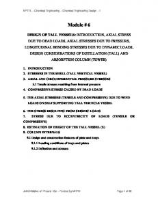
NPTEL - ADVANCED FOUNDATION ENGINEERING-1 Measuring R is difficult, but it can be estimated. Figure1.4 shows the general range of the magnitude of R with particle roundness. Figure 1.5 shows the variation of emax and emin with the uniformity coefficient for various values of particle roundness (Youd, 1973). This range is applicable to clean sand with normal to moderate skewed particle-size distribution.
Figure 1.4 General range of the magnitude of R
Figure 1.5 Approximate variation of emax and emin with uniformity coefficient (based on Youd, 1973)
NPTEL - ADVANCED FOUNDATION ENGINEERING-1 Example 1 A 0.25 ft 3 moist soil weights 30.8 lb. when dried in an oven, this soil weights 28.2 lb. givenGs = 2.7. Determine the a. b. c. d. e. f.
Moist unit weight, γ Moisture content, w Dry unit weight, γd Void ratio, e Porosity, n Degree of saturation, S
Solution
Part a. Moist Unit Weight From equation (9),
Part b. Moisture Content
γ=
w=
Part c. Dry Unit Weight
W 30.8 = = 123.2 lb/ft 3 V 0.25
Ww 30.8 − 28.2 = × 100 = 9.2% Ws 28.2
From equation (10),
Part d. Void Ratio
γd =
Ws 28.2 = = 112.8 lb/ft 3 V 0.25
From equation (4), e=
Vs =
Part e. Porosity
Vv Vs
Ws 28.2 = = 0.169 ft 3 Gs γw (2.67)(62.4) e=
0.25 − 0.169 = 0.479 0.169
From equation (6), n=
e 0.479 = = 0.324 1 + e 1 + 0.479
NPTEL - ADVANCED FOUNDATION ENGINEERING-1
Part f. Degree of Saturation From equation (7), S(%) =
Vw × 100 Vv
Vv = V − Vs = 0.25 − 0.169 = 0.081 ft 3 Vw =
Ww 30.8 − 28.2 = = 0.042 ft 3 γw 62.4
S=
Example 2
0.042 × 100 = 51.9% 0.081
A soil has a void ratio of 0.72, moisture content= 12%, and Gs = 2.72. Determine a. Dry unit weight (kN/m3 ) b. Moist unit weight (kN/m3 ) c. Weight of water in kN/m3 to be added to make the soil saturated
Solution
Part a. Dry Unit Weight From equation (12), γd =
Gs γw (2.72)(9.81) = = 15.51 kN/m3 1+e 1 + 0.72
Part b. Moist Unit Weight From equation (11), γ=
Gs γw (1 + w) (2.72)(9.81)(1 + 0.12) = = 17.38 kN/m3 1+e 1 + 0.72
Part c. Mass of Water to be Added From equation (15), γsat =
(Gs + e)γw (2.72 + 0.72)(9.81) = 19.62 kN/m3 1+e 1 + 0.72
Water to be added = γsat − γ = 19.62 − 17.38 = 2.24 kN/m3
NPTEL - ADVANCED FOUNDATION ENGINEERING-1 Example 3 The maximum and minimum dry unit weights of a sand are 17.1 kN/m3 and 14.2 kN/ m3 , respectively. The sand in the field has a relative density of 70% with a moisture content of 8%. Determine the moist unit weight of the sand in the field. Solution From equation (20), Dr = �
γd − γd(min ) γd(max ) �� � γd(max ) − γd(min ) γd
0.7 = �
γd − 14.2 17.1 �� � � 17.1 − 14.2 γd
γ = γd (1 + w) − 16.11 �1 +
ATTERBERG LIMITS
8 � = 17.4 kN/m3 100
When a clayey soil is mixed with an excessive amount of water, it may flow like a semiliquid. If the soil is gradually dried, it will behave like a plastic, semisolid, or solid material depending on its moisture content. The moisture content, in percent, at which the soil changes from a liquid to a plastic state, is defined as the liquid limit (LL). Similarly, the moisture contents, in percent, at which the soil change from a plastic to a semisolid state and from a semisolid to a solid state are define as the plastic limit (PL) and the shrinkage limit (SL), respectively. These limit a referred to as Atterberg limits (figure 1.6).
Figure 1.6 Definition of Atterberg limits The liquid limit of a soil is determined by Casegrande’s liquid device (AST Testing Designation D-4318) and is defined as the moisture content at which a groove closure of 12in. (12.7 mm) occurs at 25 blows.
NPTEL - ADVANCED FOUNDATION ENGINEERING-1 The plastic limit is defined as the moisture content at which the soil crumble when rolled into a thread of 18 in. (3.18 mm) in diameter (ASTM Testing Designation D-4318). The shrinkage limit is defined as the moisture content at which the does not undergo further volume change with loss of moisture (ASTM Testing Designation D-427). Figure 1.6 shows this limit.
The difference between the liquid limit and the plastic limit of a soil is define as the plasticity index (PI), or PI = LL − PL
[1.22]
Table 7 gives some representative values of liquid limit and plastic limit for several clay minerals and soils. However, Atterberg limits for various soils will variable considerable, depending on the soil’s origin and the nature and amount of clay minerals in it.
Table 7 Typical Liquid and Plastic Limits for Some Clay Minerals and Soils Description Kaolinite Illite Montmorillonite Boston Blue Clay Chicago clay Louisiana clay London clay Cambridge clay Montana clay Mississippi gumbo Loessial soils in north and northwest China
Liquid limit 35-100 50-100 100-800 40 60 75 66 39 52 95 25-35
Plastic limit 25-35 30-60 50-100 20 20 25 27 21 18 32 15-20
NPTEL - ADVANCED FOUNDATION ENGINEERING-1