Modulus fault attacks. Experiments and refinements. Conclusion. Modulus Fault Attacks. Against RSAâCRT Signatures. Ãric Brier1. David Naccache2. Phong Q.
Introduction
Modulus fault attacks
Experiments and refinements
Modulus Fault Attacks Against RSA–CRT Signatures ´ Brier1 David Naccache2 Eric Phong Q. Nguyen2,3 Mehdi Tibouchi2 1 Ingenico 2 Ecole ´
normale sup´ erieure 3 INRIA
CHES 2011, Nara, 2011–09–30
Conclusion
Introduction
Modulus fault attacks
Experiments and refinements
Outline
Introduction Modulus fault attacks Basic idea Using orthogonal lattices Experiments and refinements Simulation and experiments Solving the N ′ problem
Conclusion
Introduction
Modulus fault attacks
Experiments and refinements
Conclusion
Signing with RSA–CRT • RSA signatures:
σ = µ(m)d mod N For suitable padding functions µ (e.g. FDH, PSS...) this is a provably secure signature scheme. • Remains the most widely used signature scheme today.
Implemented in many embedded applications (esp. smart cards). • However, modular exponentiation is rather slow. • Very commonly used improvement: using the Chinese
Remainder Theorem. 1. σp = µ(m)d mod p−1 mod p 2. σq = µ(m)d mod q−1 mod q 3. σ = CRT(σp , σq ) mod N • Roughly 4-fold speed-up.
Introduction
Modulus fault attacks
Experiments and refinements
Conclusion
The Boneh-DeMillo-Lipton fault attack (1997) • The problem with CRT: fault attacks. • A fault in signature generation makes it possible to recover
the secret key! 1. σp = µ(m)d mod p−1 mod p 2. σq′ ≠ µ(m)d mod q−1 mod q 3. σ ′ = CRT(σp , σq′ ) mod N
← fault ← faulty signature
• Then σ ′e is µ(m) mod p but not mod q, so the attacker can
then factor N: p = gcd(σ ′e − µ(m), N) • This attack applies to any deterministic padding, including
“provably secure” ones like FDH.
Introduction
Modulus fault attacks
Experiments and refinements
Conclusion
Shamir’s trick • Faults against RSA–CRT signatures have been an active
research subject since then. Many variants and countermeasures have been proposed. • One simple countermeasure due to Shamir is to compute the signature as follows (r is a small fixed integer like 231 − 1): 1. 2. 3. 4.
σp+ = µ(m)d mod r ⋅ p σq+ = µ(m)d mod r ⋅ q if σp+ ≡/ σq+ (mod r ), abort σ = CRT(σp+ , σq+ ) mod N
• If one of the half-exponentiations is perturbed, signature
generation is very likely to abort, and hence the fault attacker cannot factor anymore!
Introduction
Modulus fault attacks
Experiments and refinements
Outline
Introduction Modulus fault attacks Basic idea Using orthogonal lattices Experiments and refinements Simulation and experiments Solving the N ′ problem
Conclusion
Introduction
Modulus fault attacks
Experiments and refinements
Conclusion
Attacking the modulus
• A lot of work has been invested into protecting the
exponentiations in RSA–CRT signature generation. • So what about attacking another part of the algorithm? • Idea: attack the modular reduction instead! 1. σp = µ(m)d mod p ← correct 2. σq = µ(m)d mod q ← correct 3. σ ′ = CRT(σp , σq ) mod N ′ ← faulty signature: wrong modular reduction! • This new, strange type of faults can also be used to factor N.
Introduction
Modulus fault attacks
Experiments and refinements
Conclusion
Using the fault (I) • More precisely, suppose we can obtain the same signature on
a certain message twice, once correctly and once with a fault. Then we get: ⎧ ⎪ ← correct ⎪σ = CRT(σp , σq ) mod N ⎨ ′ ′ ⎪ ⎪ ⎩σ = CRT(σp , σq ) mod N ← faulty • Applying the CRT to these two relations, we obtain the value CRT(σp , σq ) mod NN ′ . • Now recall that: CRT(σp , σq ) = α ⋅ σp + β ⋅ σq where α = q ⋅ (q −1 mod p)
β = p ⋅ (p −1 mod q)
• In particular, CRT(σp , σq ) is an integer of size ≈ N 3/2 , so if
we know it modulo NN ′ ≈ N 2 , we actually know its value in Z.
Introduction
Modulus fault attacks
Experiments and refinements
Conclusion
Using the fault (II) Each pair formed of a correct and of a faulty signature gives us an equation of the form: v =α⋅x +β⋅y where v is known, α, β are unknown, fixed and of size N, and x, y are unknown, of size N 1/2 , and depend on the signature. One such relation doesn’t get us far, but since (x, y ) is small compared to (α, β), we expect multiple relations of this form to allow us to recover the x’s and y ’s, and hence factor N. So suppose we can obtain a vector v of ` CRT values, so that we have an equation: v = αx + βy The goal is to recover x and y from v. To do so, we can used a cryptanlytic technique introduced by Nguyen and Stern in the 1990s: orthogonal lattices.
Introduction
Modulus fault attacks
Experiments and refinements
Outline
Introduction Modulus fault attacks Basic idea Using orthogonal lattices Experiments and refinements Simulation and experiments Solving the N ′ problem
Conclusion
Introduction
Modulus fault attacks
Experiments and refinements
A primer on lattices
A lattice L is a subgroup of Zn for some n: a regular arrangement of points in Rn .
Conclusion
Introduction
Modulus fault attacks
Experiments and refinements
A primer on lattices
Often represented by a basis (minimal generating set of vectors in L).
Conclusion
Introduction
Modulus fault attacks
Experiments and refinements
A primer on lattices
dim(L) = 2
The number of vectors in a basis is called the rank or dimension dim(L). It is well-defined.
Conclusion
Introduction
Modulus fault attacks
Experiments and refinements
A primer on lattices
dim(L) = 1
The number of vectors in a basis is called the rank or dimension dim(L). It is well-defined.
Conclusion
Introduction
Modulus fault attacks
Experiments and refinements
A primer on lattices
dim(L) = 2
The number of vectors in a basis is called the rank or dimension dim(L). It is well-defined.
Conclusion
Introduction
Modulus fault attacks
Experiments and refinements
Conclusion
A primer on lattices
Some bases are better than others: with shorter, almost orthogonal vectors. We call them reduced basis.
Introduction
Modulus fault attacks
Experiments and refinements
Conclusion
A primer on lattices
We have algorithms, such as LLL, to compute reduced bases. In low dimension (say ≲ 100), we can obtain “optimal” lattice reduction in practice.
Introduction
Modulus fault attacks
Experiments and refinements
Conclusion
A primer on lattices
vol(L) = 7
Another important invariant: lattice volume; d-dimensional volume of the parallelipiped defined by a basis. Independent of the basis.
Introduction
Modulus fault attacks
Experiments and refinements
Conclusion
A primer on lattices
vol(L) = 7
Another important invariant: lattice volume; d-dimensional volume of the parallelipiped defined by a basis. Independent of the basis.
Introduction
Modulus fault attacks
Experiments and refinements
Conclusion
A primer on lattices
vol(L)1/2 ≈ 2.6
2.2 3.2
For “typical” (e.g. random) lattices, vectors in a short basis are all roughly the same length ≈ vol(L)1/ dim(L) .
Introduction
Modulus fault attacks
Experiments and refinements
A primer on lattices
Given a lattice L of dimension d in Zn , the set of vectors in Zn orthogonal to all of the vectors in L is also a lattice L⊥ , of dimension n − d and volume vol(L⊥ ) = vol(L).
Conclusion
Introduction
Modulus fault attacks
Experiments and refinements
Conclusion
A primer on lattices
Given a basis of L, we can compute a reduced basis of L⊥ using an algorithm due to Nguyen and Stern (LLL in dimension n + d).
Introduction
Modulus fault attacks
Experiments and refinements
Conclusion
A primer on lattices
Given a basis of L, we can compute a reduced basis of L⊥ using an algorithm due to Nguyen and Stern (LLL in dimension n + d).
Introduction
Modulus fault attacks
Experiments and refinements
Conclusion
Lattice attack overview (I) • Recall that we have a vector v = αx + βy in Z` with x, y
unknown. We want to recover these hidden vectors. Let L = Zv ⊂ Z` . • Compute a reduced basis (b1 , . . . , b`−1 ) of the lattice L⊥ of vectors in Z` orthogonal to v. The volume of this lattice is vol(L⊥ ) = vol(L) = ∥v∥ ≈ N 3/2 • Since v = αx + βy, the bi ’s satisfy:
α⟨bi , x⟩ + β⟨bi , y⟩ = 0 • But the smallest nonzero solution (s, t) to αs + βt = 0 is of
size ≈ N, so a given √ bi is either orthogonal to both x and y, or it is of norm > N. • Only ` − 2 independent vectors orthogonal to both x and y, so √ b`−1 must be of length > N. The remaining vectors b1 , . . . , b`−2 generate a lattice L′ of volume ≈ vol(L)/∥b`−1 ∥ ≈ N.
Introduction
Modulus fault attacks
Experiments and refinements
Conclusion
Lattice attack overview (II) • Since L′ has no reason to be special, assume heuristically that
it behaves like a random lattice. In particular, we expect all of the vectors in the reduced basis (b1 , . . . , b`−2 to be roughly of length vol(L′ )1/(`−2) ≈ N 1/(`−2) . √ • In particular, if ` ≥ 5, they are all of length ≪ N. Therefore, they are orthogonal to x, y. • Then, compute a reduced basis (x′ , y′ ) of the orthogonal
lattice (L′ )⊥ . This lattice is of volume vol(L′ ) ≈ N, and √ in particular doesn’t contain many vectors of length ≤ `N (we can enumerate them easily). But x is one of them! √ • For each pair (s, t) such that z = sx′ + ty′ is of length ≤ `N, compute gcd(v − z, N). When we reach z = x, this GCD is p, because v is equal to x mod p but not mod q. • Hence, we have factored N (provided that ` ≥ 5)!
Introduction
Modulus fault attacks
Experiments and refinements
Conclusion
Lattice attack overview (II) • Since L′ has no reason to be special, assume heuristically that
• •
•
•
it behaves like a random lattice. In particular, we expect all of the vectors in the reduced basis (b1 , . . . , b`−2 to be roughly of length vol(L′ )1/(`−2) ≈ N 1/(`−2) . √ In particular, if ` ≥ 5, they are all of length ≪ N. Therefore, they are orthogonal to x, y. Then, compute a reduced basis (x′ , y′ ) of the orthogonal lattice (L′ )⊥ . This lattice is of volume vol(L′ ) ≈ N, and √ in particular doesn’t contain many vectors of length ≤ `N (we can enumerate them easily). But x is one of them! √ For each pair (s, t) such that z = sx′ + ty′ is of length ≤ `N, compute gcd(v − z, N). When we reach z = x, this GCD is p, because v is equal to x mod p but not mod q. Hence, we have factored N (provided that ` ≥ 5)! (At least heuristically).
Introduction
Modulus fault attacks
Experiments and refinements
Outline
Introduction Modulus fault attacks Basic idea Using orthogonal lattices Experiments and refinements Simulation and experiments Solving the N ′ problem
Conclusion
Introduction
Modulus fault attacks
Experiments and refinements
Conclusion
Simulation of the attack Since the attack is heuristic, validation is in order. Simulate the attack as follows: • Pick random p, q-parts (xi , yi ). • Compute the corresponding CRT values vi in Z. • Try to factor N using the orthogonal lattice attack. Namely: 1. Compute a reduced basis (b1 , . . . , b`−1 ) of the orthogonal lattice of Zv) with LLL. 2. Compute a reduced basis (x′ , y′ ) of the orthogonal lattice of Zb1 ⊕ ⋯ ⊕ Zb`−2 . √ 3. Enumerate the vectors z of Zx′ ⊕ Zy′ of length at most `N and compute the GCDs gcd(v − z, N) until a factor is found.
Introduction
Modulus fault attacks
Experiments and refinements
Conclusion
Simulation results Number of faulty signatures ` 4 5 6 1024-bit moduli 48% 100% 100% 1536-bit moduli 45% 100% 100% 2048-bit moduli 46% 100% 100% Success probability of the attack with various parameters. Modulus size 1024 1536 Average search space π`N/V 24 23 Average total CPU time 16 ms 26 ms Efficiency of the attack with ` = 5.
2048 24 34 ms
Introduction
Modulus fault attacks
Experiments and refinements
Conclusion
The attack in practice We carried out the attack against an implementation of RSA–CRT signatures on an unprotected 8-bit microcontroller. 1. Decapsulate the chip. 2. Target the SRAM and find the location of the modulus N. 3. Strike with 4. After obtaining 5 pairs of correct and faulty signatures, factor N in a fraction of a second as expected.
Introduction
Modulus fault attacks
Experiments and refinements
Conclusion
The attack in practice We carried out the attack against an implementation of RSA–CRT signatures on an unprotected 8-bit microcontroller. 1. Decapsulate the chip.
2. Target the SRAM and find the location of the modulus N. 3. Strike with 4. After obtaining 5 pairs of correct and faulty signatures, factor N in a fraction of a second as expected.
Introduction
Modulus fault attacks
Experiments and refinements
Conclusion
The attack in practice We carried out the attack against an implementation of RSA–CRT signatures on an unprotected 8-bit microcontroller. 1. Decapsulate the chip. 2. Target the SRAM and find the location of the modulus N.
3. Strike with 4. After obtaining 5 pairs of correct and faulty signatures, factor N in a fraction of a second as expected.
Introduction
Modulus fault attacks
Experiments and refinements
Conclusion
The attack in practice We carried out the attack against an implementation of RSA–CRT signatures on an unprotected 8-bit microcontroller. 1. Decapsulate the chip. 2. Target the SRAM and find the location of the modulus N. 3. Strike with lasers!
4. After obtaining 5 pairs of correct and faulty signatures, factor N in a fraction of a second as expected.
Introduction
Modulus fault attacks
Experiments and refinements
Conclusion
The attack in practice We carried out the attack against an implementation of RSA–CRT signatures on an unprotected 8-bit microcontroller. 1. Decapsulate the chip. 2. Target the SRAM and find the location of the modulus N. 3. Strike with a focused laser beam.
4. After obtaining 5 pairs of correct and faulty signatures, factor N in a fraction of a second as expected.
Introduction
Modulus fault attacks
Experiments and refinements
Conclusion
The attack in practice We carried out the attack against an implementation of RSA–CRT signatures on an unprotected 8-bit microcontroller. 1. Decapsulate the chip. 2. Target the SRAM and find the location of the modulus N. 3. Strike with 4. After obtaining 5 pairs of correct and faulty signatures, factor N in a fraction of a second as expected.
Introduction
Modulus fault attacks
Experiments and refinements
Outline
Introduction Modulus fault attacks Basic idea Using orthogonal lattices Experiments and refinements Simulation and experiments Solving the N ′ problem
Conclusion
Introduction
Modulus fault attacks
Experiments and refinements
Conclusion
Problem with the faulty moduli • Earlier, I claimed that to obtain the CRT values vi in Z, we
• • • •
needed pairs (σi , σi′ ) formed of a correct and a faulty signature on the same message. But this is not enough: to compute vi = CRT(σi , σi′ ), one needs to know the faulty modulus Ni′ . Not very realistic: the signing device is unlikely to output its public modulus together with a signature. Fortunately, with a few more faulty of a certain reasonable shape, we can find the vi ’s without knowing the faulty moduli. We give solutions under the following two fault models: 1. Single-byte faults: the faulty moduli Ni′ only differ from N on 8 consecutive bits (e.g. glitch attack when copying the modulus from memory on an 8-bit architecture). 2. LSB faults: the faulty moduli Ni′ only differ from N on the least significant half of all bits (e.g. laser beam targeted at the LSBs of N in memory).
Introduction
Modulus fault attacks
Experiments and refinements
Solution for LSB faults (I) • Suppose that, on a given message m, we can obtain not a
correct-faulty signature pair (σ, σ ′ ), but several faulty signatures σj′ , 1 ≤ j ≤ k corresponding to unknown faulty √ moduli Nj′ = N + εj (∣εj ∣ ≪ N). • Given this data, we want to recover the CRT value v in Z. • We can write: v = σ + t0 ⋅ N = σj′ + tj ⋅ (N + εj ) √ for some integers tj of size N. • Hence, for 1 ≤ j ≤ k, σ − σj′ ≡ tj εj (mod N), and since ∣tj εj ∣ ≪ N, the equality holds in Z. • As a result, we get tj = t0 for all j, and hence: σ − σj′ = t0 ⋅ εj • If gcd(ε1 , . . . , εk ) = 1, we can compute t0 as
gcd(σ − σ1′ , . . . , σ − σj′ ), and deduce v accordingly.
Conclusion
Introduction
Modulus fault attacks
Experiments and refinements
Conclusion
Solution for LSB faults (II) • The probability that this method works is the probability that
ε1 , . . . , εk are coprime, namely 1/ζ(k). This converges quickly to 1 as k grows, and this theoretical value is verified very well in simulation. • Since we need ` = 5 CRT values to carry out the lattice
attack, this method requires k ⋅ ` faulty signatures overall and has a success probability of ζ(k)−` . • Taking ` = 5, k = 9 (45 faults in total) gives a success
probability > 99%. • Validated experimentally using laser fault injection, even with
k as low as 4 (theoretical success probability of 67%)!
Introduction
Modulus fault attacks
Experiments and refinements
Conclusion
Conclusion • This new attack presents a number of nice features: • Quite efficient and doesn’t require too many faults (45 faulty signatures enough in a typical setting for > 99% success rate). • Not thwarted by e.g. Shamir’s trick. • However, it does have some limitations: • Must be able to obtain a correct and a faulty signature with the same CRT value: not possible with probabilistic paddings like PSS. • Most seriously: a faster, frequently used technique for CRT interpolation (Garner’s formula) avoids reducing mod N altogether, and hence defeats this attack. • Possible extension to protected RSA–CRT implementations
that do a final modular reduction? To discrete log settings?
Introduction
Modulus fault attacks
Experiments and refinements
Thank you!
Conclusion