Atmos. Chem. Phys., 10, 5707–5718, 2010 www.atmos-chem-phys.net/10/5707/2010/ doi:10.5194/acp-10-5707-2010 © Author(s) 2010. CC Attribution 3.0 License.
Atmospheric Chemistry and Physics
Molecular hydrogen (H2) emissions and their isotopic signatures (H/D) from a motor vehicle: implications on atmospheric H2 M. K. Vollmer1 , S. Walter2 , S. W. Bond1 , P. Soltic3 , and T. R¨ockmann2 1 Empa,
Swiss Federal Laboratories for Materials Science and Research, Laboratory for Air Pollution and Environmental ¨ Technology, Uberlandstrasse 129, 8600 D¨ubendorf, Switzerland 2 Institute for Marine and Atmospheric research Utrecht, Utrecht University, Princetonplein 5, 3508TA Utrecht, The Netherlands 3 Empa, Swiss Federal Laboratories for Materials Science and Research, Laboratory of I. C. Engines, Uberlandstrasse ¨ 129, 8600 D¨ubendorf, Switzerland Received: 24 November 2009 – Published in Atmos. Chem. Phys. Discuss.: 5 February 2010 Revised: 26 May 2010 – Accepted: 10 June 2010 – Published: 29 June 2010
Abstract. Molecular hydrogen (H2 ), its isotopic signature (deuterium/hydrogen, δD), carbon monoxide (CO), and other compounds were studied in the exhaust of a passenger car engine fuelled with gasoline or methane and run under variable air-fuel ratios and operating modes. H2 and CO concentrations were largely reduced downstream of the three-way catalytic converter (TWC) compared to levels upstream, and showed a strong dependence on the air-fuel ratio (expressed as lambda, λ). The isotopic composition of H2 ranged from δD=−140‰ to δD = −195‰ upstream of the TWC but these values decreased to −270‰ to −370‰ after passing through the TWC. Post-TWC δD values for the fuelrich range showed a strong dependence on TWC temperature with more negative δD for lower temperatures. These effects are attributed to a rapid temperature-dependent H-D isotope equilibration between H2 and water (H2 O). In addition, post TWC δD in H2 showed a strong dependence on the fraction of removed H2 , suggesting isotopic enrichment during catalytic removal of H2 with enrichment factors (ε) ranging from −39.8‰ to −15.5‰ depending on the operating mode. Our results imply that there may be considerable variability in real-world δD emissions from vehicle exhaust, which may mainly depend on TWC technology and exhaust temperature regime. This variability is suggestive of a δD from traffic that varies over time, by season, and by geographical location. An earlier-derived integrated pure (end-member) δD from anthropogenic activities of −270‰ (Rahn et al., 2002)
Correspondence to: M. K. Vollmer (
[email protected])
can be explained as a mixture of mainly vehicle emissions from cold starts and fully functional TWCs, but enhanced δD values by >50‰ are likely for regions where TWC technology is not fully implemented. Our results also suggest that a full hydrogen isotope analysis on fuel and exhaust gas may greatly aid at understanding process-level reactions in the exhaust gas, in particular in the TWC.
1
Introduction
The poorly understood budget of atmospheric molecular hydrogen (H2 ) has received increased attention over the past years because of a potentially massive disturbance in the near future due to a potential shift towards a hydrogen energy economy. Recent studies have revealed potential negative impacts on stratospheric ozone and on earth’s climate systems via the role of H2 in atmospheric chemistry; however, quantitative estimates are highly uncertain, largely due to unknown leakage rates of H2 to the atmosphere from future H2 energy systems. In the traffic sector, current H2 emissions from conventional combustion engine systems would disappear, but could be replaced by leakage and purged losses from H2 -powered vehicles. H2 is abundant in the atmosphere at relatively high concentrations (hereafter expressed as dry air mole fraction) of 450 ppb – 550 ppb (parts-per-billion, 10−9 , molar). Its source and sink strengths are given here as ranges found in the literature (Novelli et al., 1999; Hauglustaine and Ehhalt, 2002; Sanderson et al., 2003; Rhee et al., 2006; Price et al., 2007; Xiao et al., 2007; Ehhalt and Rohrer, 2009): The major
Published by Copernicus Publications on behalf of the European Geosciences Union.
5708 sources are in-situ photochemical production from methane (CH4 ) and other hydrocarbons (30–77 Tg a−1 ), fossil fuel emissions (11–20 Tg a−1 ), biomass burning (10 – 20 Tg a−1 ), and minor emissions from microbial nitrogen (N2 ) fixation on land and in the oceans (6–10 Tg a−1 ). The dominant sink of H2 is enzymatic destruction in soil (55–88 Tg a−1 ), but there is also considerable removal through oxidation by the hydroxyl radical in the atmosphere (15–19 Tg a−1 ). These fluxes result in a tropospheric lifetime of H2 of 1.4–2.2 a. Due to the dominant soil sink and the larger land coverage in the Northern Hemisphere, this hemisphere exhibits smaller tropospheric concentrations compared to the Southern Hemisphere, which is an unusual distribution for atmospheric trace gases. Stable isotope measurements of H2 using the hydrogen/deuterium (H/D) ratio have greatly added to differentiating various sources and sinks (Brenninkmeijer et al., 2003; Ehhalt and Rohrer, 2009). This is particularly true because of largely differing isotopic signatures of the sources. For example, H2 from CH4 oxidation is particularly enriched in deuterium with δD values ∼130‰ to 180‰ (Rahn et al., 2003; Rhee et al., 2006; Feilberg et al., 2007; R¨ockmann et al., 2003; Pieterse et al., 2009), biogenic H2 is extraordinarily depleted (δD ∼ −700‰, e.g. Rahn et al. (2002); Walter and et al. (2010)), and combustion-derived H2 has δD values of approximately −170‰ to −270‰ (Gerst and Quay, 2001; Rahn et al., 2002). Automobile exhaust is believed to dominate anthropogenic H2 emissions, and has recently been estimated globally at 4.2–5.4 Tg a−1 with a decreasing trend, based on a fleet-integrated tunnel emission study (Vollmer et al., 2007). The single available isotope study of regional traffic emissions using polluted air samples from the Los Angeles basin by Rahn et al. (2002) suggests an urban pollution isotopic signature of −270‰ for this region. Samples taken near the exhaust of individual vehicles in their study showed considerable variability in the isotopic signature, as did a few samples collected in a parking garage by Gerst and Quay (2001), which showed less depleted δD. Engine and catalytic converter technology is evolving rapidly, and along with the increasing diversity of fuel types, presents a challenge for vehicle emissions characterization. Such studies can be conducted on various levels of detail, and range from regional scale atmospheric observations of polluted air masses to single unit process studies. Isotope investigations can greatly improve the distinction from other sources and sinks of pollutants. For vehicle exhaust, progress has recently been achieved through isotopic studies of e.g. carbon monoxide, CO (Tsunogai et al., 2003), methane, CH4 (Chanton et al., 2000; Nakagawa et al., 2005), and nitrous oxide, N2 O (Toyoda et al., 2008). Here we present results from a study on a passenger car engine for which we have measured pre- and post-catalytic H2 concentrations and – to our knowledge for the first time – H/D signatures under variable engine and fuel settings. Atmos. Chem. Phys., 10, 5707–5718, 2010
M. K. Vollmer et al.: Molecular hydrogen from traffic 2 2.1
Materials and methods Experimental setup
The engine experiment was conducted in 2008 on an engine test bench at the Empa Internal Combustion Engines Laboratory using a naturally-aspirated passenger car engine with four cylinders, 2-L displacement, and the capability to combust either gasoline or natural gas. The engine was equipped with a state-of-the art engine control unit, which was originally calibrated to achieve Euro-4 emission limits for a midsize passenger car. On the test bench, the control parameters could be modified to study e.g. the influence of the air-tofuel ratio on combustion and emissions. The combustion air fed to the engine was conditioned to a temperature of 295 K and a relative humidity of 50%. The exhaust system was equipped with a single three-way ceramic substrate catalytic converter (TWC) with a cell density of 600 cells per square inch (cpsi) and coated with palladium and rhodium as the catalytically active materials. Ceria, an oxide of the element cerium, was used in the TWC’s wash-coat to achieve the desired oxygen storage capacity. For the sake of the later temperature discussion, it is worthy to mention that a TWC is not actively heated but that it is initially cold (termed “cold start” in traffic studies) after engine start-up until sufficient hot exhaust gas passes through it to make it fully functional (light-off temperature). For air-to-fuel ratio feedback control, the engine was equipped with a linear lambda (λ) sensor upstream of the catalyst and a switching-type λ sensor downstream of the TWC for bias control. Linear λ sensors are able to measure deviations of λ very precisely but they unfortunately show a relatively slow signal drift, which depends on many factors. To compensate for this drift, the bias of the linear λ sensor is corrected occasionally using the signal of a much simpler switching-type λ sensor mounted downstream of the TWC. Such switching-type sensors show a very stable and steep signal change at λ=1 but no useful information of the actual λ value in fuel-rich or fuel-lean operating conditions. The engine control used a square signal “λ-wobbling” function with an amplitude of 0.02 to the nominal λ setting. These rich-lean excursions are very often used in modern engine controls to enhance the TWC’s efficiency, and to perform diagnosis of the TWC during engine operation using the TWC’s dynamic response to this wobbling. The experiment was conducted for 4 different operating modes (OMs) as is shown in Table 1, where OM-1 used the same engine settings as OM-2, but in the first case the TWC was cooled by active air ventilation of the exhaust manifold and the piping upstream of the TWC. All OMs reflect relatively low engine power, which are frequently used in normal operations of passenger cars. OM-2 is a standard setting, which is widely used in engine research for comparative purposes. OM-3 and OM-4 differ from OM-2 in torque and crankshaft speed and represent low revolution per minute (rpm) and high-rpm driving, both at double the engine power www.atmos-chem-phys.net/10/5707/2010/
M. K. Vollmer et al.: Molecular hydrogen from traffic
5709
Table 1. Operating modes (OM) for the experiments conducted on a passenger car engine. The three-way catalytic converter (TWC) was actively cooled in operating mode 1. OM-1 through OM-4 are gasoline-fuelled, OM-3-CH4 is methane-fuelled. Upstream and downstream TWC temperatures are lambda-dependent (low temperatures for low lambda). Although the TWC is not actively heated, some downstream temperatures are higher due to exothermic reactions occurring within the TWC. Operating Mode (OM) OM-1 OM-2 OM-3 OM-4 OM-3-CH4
Crankshaft speed [r.p.m]
Torque
Power
[N m]
[kW]
2000 2000 2000 4000 2000
31.6 31.6 63.2 31.6 63.2
6.6 6.6 13.2 13.2 13.2
Downstream TWC cooling
Upstream TWC temperature range [◦ C]
Downstream TWC temperature range [◦ C]
yes no no no no
460–490 530–556 598–629 690–721 566–590
456–534 512–586 566–642 665–753 558–620
of OM-1 and OM-2. In order to study the air-to-fuel settings on the pollutant emissions before and after TWC, the λ for each OM was varied around λ = 1.0. To prevent undesired fuelling changes caused by a λ bias control, bias control was turned off. The gasoline used for these experiments was market fuel with research octane number 95.5, a density of 736 kg m−3 , a sulphur content of 22.6 mg kg−1 , and an H/C ratio of 1.97. One of the purposes of this experiment was to study the interference of H2 in the exhaust on the lambda probe. For this reason all operating modes were repeated using CH4 as the engine fuel (commercial bottled CH4 based on fossil-fuel natural gas). However, the focus of the H2 stable isotope study was on the exhaust of the gasoline-powered engine, and we therefore discuss the CH4 results only briefly in the context of the H2 isotopes. In addition to the chemical species discussed here, measurements in the exhaust were made of O2 , nitrogen oxides (NOx , NO, NO2 ), CH4 , shortchained hydrocarbons (C2 –C4 ), some aromatics, total hydrocarbons (HC), water (H2 O), N2 O, and sulphur dioxide (SO2 ). Samples for D/H isotope analysis were collected at ∼2 bar in 1-L glass flasks fitted with 2 stopcocks (NORMAG, Illmenau, Germany), and others at ∼3 bar in ∼2-L internally electro-polished stainless steel (ss) canisters using a small membrane pump (KNF model N86-KTE). The sampling stream was cooled in an ice bath before entering the pump and the condensed water was periodically removed. The samples were further dried using magnesium perchlorate (Mg(ClO4 )2 ) before collection in the flasks. Analysis of the samples was performed within 3 months after their collection. 2.2
Instrumentation
H2 concentrations were measured on-line using a commercially available electron impact ionization mass spectrometer (EIMS, H-Sense, V&F Analyse und Messtechnik, Absam, Austria). The instrument precision is ∼1% (1σ of 1min mean). However the measurements were affected by a blank of ∼8 ppm (parts-per-million, 10−6 , molar), likely www.atmos-chem-phys.net/10/5707/2010/
caused by some H2 O interference in the system. This blank was determined and corrected for by comparing the EIMS results with the concentration results from the flask samples, which were available for the low-concentration range (λ >1). While this blank correction is of little relevance for the highconcentration samples, it resulted in considerable uncertainties of up to 50% for some of the low-concentration samples. Calibration of the instrument was achieved using commercial standards (30 ppm and 1000 ppm, Messer Schweiz, accuracies 0.5%) and during an independent validation study, the instrument was found to exhibit linear response within the range of our measured concentrations (Br¨uhlmann, 2004). Overall accuracies of the H2 concentrations are estimated at 5 ppm or 3%, whichever is greater. CO, CO2 , and H2 O were measured on-line using an automotive Fourier Transformation Infra-red (FTIR) instrument (AVL SESAM). This instrument was calibrated during commissioning using high-precision gases and did not need recalibration during the experiment. Estimated uncertainties are 0.14% for H2 O, 0.12% for CO and 0.33% for CO2 . The CO and CO2 concentrations were converted to dry air mole fractions using this instrument’s H2 O results. Earliermentioned compounds, which are not discussed here, were also measured on this FTIR and on a standard engine emission bench instrument (Horiba Mexa 9200). Isotopic measurements of H2 from the flask samples were conducted in the isotope laboratory of the Institute for Marine and Atmospheric research Utrecht (IMAU), Utrecht University using isotope ratio mass spectrometry (Rhee et al., 2004). Isotope results are reported using the “delta” notation, δD = [(D/H)s /(D/H)VSMOW −1]×1000‰, where s is the H2 of the sample and VSMOW is Vienna standard mean ocean water used as reference (Craig, 1961; Gonfiantini, 1978). The mean of the 1-σ precisions from repeated analysis and duplicate samples is 11‰, which is poorer than for ambient air measurements and caused by the high concentrations employed in this study.
Atmos. Chem. Phys., 10, 5707–5718, 2010
5710 2.3
M. K. Vollmer et al.: Molecular hydrogen from traffic Results and discussion
H2/CO (molar)
CO concentration [ × 103 ppm ]
δD in H2 [ %o ]
3
H2 concentration [ × 10 ppm ]
The results for our compounds of interest are listed in Table 2 7 OM−4 a) and shown in Fig. 1 as a function of the air-fuel ratio. The airOM−3 6 OM−2 fuel ratio is expressed here as a lambda (λ) value, whereby OM−1 5 OM−3−CH4 λ 1 corresponds to fuel-lean combustion (excess oxygen present). H2 and CO are pro3 duced during incomplete combustion, and their abundance is 2 related, amongst other chemical reactions, through the water1 gas shift reaction H2 + CO2 ↔ H2 O + CO. Pre-TWC results 0 showed largest emissions under fuel-rich conditions, with concentrations up to ∼14 000 ppm for H2 and ∼41 000 ppm fuel−rich fuel−lean for CO. These concentrations decreased with increasing λ to −100 about 1000–1500 ppm for H2 and 4000–7000 ppm for CO b) for the leanest samples. From the presence of large H2 con−150 centrations in all pre-TWC samples, we conclude that the H2 −200 concentration and isotope ratio in the intake air (which we −250 measured in a nearby ambient sample with a concentration −300 of 573 ppb and a δD of 83.3‰) is not relevant in the following discussion. −350 Post-TWC emissions of H2 and CO were lower compared −400 to the pre-TWC emissions. Here the emissions were also larger in the fuel rich range, but nearly disappeared in the 20 c) fuel-lean range. For H2 , most concentrations of the fuel-lean experiments were below typical ambient atmospheric values 15 of ∼0.5 ppm, implying that under these conditions, H2 is de10 stroyed on the TWC. The post-TWC H2 concentrations in the fuel-rich range were highly dependent on the operating 5 mode, with highest emissions for OM-4. In contrast, the post-TWC concentrations for CO showed remarkably sim0 ilar λ dependence for all 4 operating modes. The cooling of the TWC also had significant effects on 1.6 d) post-TWC H2 emissions. The reduction of the TWC temper1.4 atures in OM-1 by ∼ 50 ◦ C compared to OM-2 (Table 1) re1.2 sulted in a reduction of H2 emissions to less than half of those 1 in the fuel-rich range, but had no effect on the CO emissions. 0.8 These observations demonstrate that reactions other than the 0.6 water-gas-shift play a role, because the latter alone would be 0.4 driving the equilibrium to higher H2 yield at reduced tem0.2 peratures (Haryanto et al., 2009), and not the opposite we’ve 0 observed. One possible explanation for these observations 0.94 0.96 0.98 1 1.02 is that the TWC’s active sites are occupied by hydrocarbons air−fuel ratio λ [ ] thereby preventing adsorption of H2 O required for the watergas-shift reaction (e.g. Auckenthaler, 2005). Our D/H isotope analysis shows largely differing isotope Fig. 1. Engine exhaust concentrations for H2 (a) and its isotope Engine exhaustratio concentrations and its H isotope ratio δD (b), CO (c), and the ratio H 2 (a) δD (b), COfor (c),Hand the ratio ratios between the individual settings, withFig. the1.following 2 /CO (d) vs. the air-fuel ratio (λ)upstream upstream(open (opensymbols) symbols)and anddownstream downstream(filled (filledsymbols) symbols)ofofthe three-way the air-fuel three major observations. Firstly, for a givenvs.air-fuel ratio,ratio (λ) the three-way catalytic (TWC) converter. The colors differentiate the H2 in the post-TWC exhaust was more depleted in deu(TWC) converter. The colors differentiate the four main operating modes of the gasoline-fuelled engin the four main operating modes of the gasoline-fuelled engine and terium compared to the pre-TWC exhaust. For the range isotope results for one the methane-fuelled mode in (b). Theoperating data for the lowest λ are omitted to isotope resultsoperating for one methane-fuelled mode in (b). where pre- and post-TWC samples were available, the preThe data for the lowest λ are omitted to show the remaining results remaining TWC δD values ranged from −140‰ to −195‰ but results these in closer detail. Vertical and horizontal dashed lines are visual aids at λ=1 and zero in closer detail. Vertical and horizontal dashed lines are visual aids values decreased to between −270‰ and −370‰ after passrespectively. at λ=1 and zero y-values, respectively. ing through the TWC. Secondly, the post-TWC D/H ratios showed a strong dependence on λ with lower δD in the fuelAtmos. Chem. Phys., 10, 5707–5718, 2010
18 www.atmos-chem-phys.net/10/5707/2010/
M. K. Vollmer et al.: Molecular hydrogen from traffic
5711
Table 2. Temperatures, trace gas concentrations, and H2 isotope ratio for pre-TWC (three-way catalytic converter) and post-TWC exhaust gasoline and from a methane-fuelled engine. The operating modes (OM) OM 1–4 are gasoline fuelled and OM 3-CH4 is methane fuelled. These OM are further specified in Table 1. Pre-TWC Operating Mode
Lambda []
1 1 1 1 1 1 1 1 1 1 1 1 1 1 1 2 2 2 2 2 2 2 2 2 2 2 2 2 2 2 3 3 3 3 3 3 3 3 3 3 3 3 3 3 3 4 4 4 4 4 4 4 4 4 4 4 4 4 4 4 3-CH4 3-CH4 3-CH4 3-CH4 3-CH4 3-CH4 3-CH4 3-CH4 3-CH4 3-CH4 3-CH4 3-CH4 3-CH4 3-CH4 3-CH4
0.892 0.942 0.972 0.982 0.984 0.986 0.988 0.990 0.992 0.994 0.996 0.998 1.000 1.002 1.012 0.892 0.942 0.972 0.982 0.984 0.986 0.988 0.990 0.992 0.994 0.996 0.998 1.000 1.002 1.012 0.894 0.944 0.974 0.984 0.986 0.988 0.990 0.992 0.994 0.996 0.998 1.000 1.002 1.004 1.014 0.896 0.946 0.976 0.986 0.988 0.990 0.992 0.994 0.996 0.998 1.000 1.002 1.004 1.006 1.016 0.902 0.952 0.982 0.992 0.994 0.996 0.998 1.000 1.002 1.004 1.006 1.008 1.010 1.012 1.022
Temp. [◦ C] 466 481 485 487 487 488 488 488 490 489 490 490 490 490 491 530 545 551 553 554 553 555 553 555 553 555 555 556 555 555 598 616 620 624 623 623 625 625 625 625 627 625 626 626 629 690 710 715 717 719 717 718 719 719 720 719 720 721 720 720 566 583 588 589 590 588 589 588 588 590 588 589 586 586 587
H2 conc. [103 ppm] 13.91 6.52 3.88 3.12 2.99 2.87 2.73 2.65 2.57 2.40 2.26 2.15 2.05 1.98 1.50 13.92 6.50 3.81 3.03 2.88 2.78 2.68 2.54 2.44 2.31 2.17 2.08 1.99 1.83 1.43 13.25 5.86 3.25 2.58 2.45 2.33 2.18 2.05 1.96 1.83 1.72 1.59 1.52 1.44 0.98 13.93 6.57 4.04 3.25 3.13 2.99 2.81 2.70 2.62 2.44 2.35 2.18 2.07 1.98 1.54 24.35 12.33 6.33 4.92 4.64 4.41 3.96 3.70 3.50 3.34 3.08 3.05 2.80 2.69 1.93
www.atmos-chem-phys.net/10/5707/2010/
δD-H2 [‰] – – – – – – – – –141 – – – – – – – – – – – – – – –173 – – – – – – – – – – – – – – –195 – – – – – – – – – – – – – – –163 – – – – – – – – – – – – – – – – – – – – –
Post-TWC
CO conc. [103 ppm] 38.86 18.93 11.63 9.60 9.26 9.01 8.64 8.61 8.41 8.17 7.94 7.59 7.30 7.13 5.71 39.18 18.89 11.78 9.56 9.28 9.04 8.87 8.55 8.35 8.14 7.89 7.67 7.45 6.90 5.71 38.96 18.45 10.80 8.85 8.55 8.24 7.96 7.71 7.36 7.02 6.70 6.16 5.95 5.74 4.22 41.39 20.73 13.50 11.32 11.08 10.67 10.15 9.89 9.44 9.18 8.97 8.63 8.43 8.28 7.04 35.52 19.46 10.99 9.20 8.97 8.62 8.25 7.79 7.39 7.19 6.69 6.75 6.20 5.97 4.53
CO2 conc. [103 ppm]
Temp. [◦ C]
122 139 145 146 146 146 147 147 147 147 147 147 147 147 148 122 139 145 146 146 146 147 147 147 147 147 147 147 147 147 123 140 146 148 148 148 148 148 149 149 149 149 149 150 149 120 139 143 145 145 145 145 146 146 146 146 146 146 147 147 88 102 108 110 111 110 111 110 110 111 111 111 110 110 110
456 483 504 513 515 517 520 523 525 528 530 532 534 531 521 512 537 556 563 566 567 569 571 576 576 581 580 586 580 570 568 596 616 627 627 629 632 633 634 638 640 638 638 635 626 668 701 725 737 739 741 743 745 749 750 753 751 748 745 735 567 586 608 618 617 620 620 615 609 603 596 589 590 581 571
H2 conc [103 ppm]
δD-H2 [‰]
CO conc. [103 ppm]
9.37 0.79 0.42 0.36 0.34 0.32 0.29 0.26 0.22 0.17 0.11 0.06 0.02 0.00 0.00 9.58 2.44 2.42 1.51 1.17 0.87 0.69 0.56 0.48 0.35 0.26 0.14 0.02 0.00 0.00 9.89 2.02 1.23 0.96 0.88 0.78 0.69 0.57 0.46 0.35 0.13 0.00 0.00 0.00 0.00 14.00 5.32 3.02 2.04 1.78 1.50 1.24 0.92 0.64 0.30 0.04 0.00 0.00 0.00 0.00 19.32 3.74 0.76 0.21 0.13 0.09 0.15 0.00 0.00 0.00 0.00 0.00 0.00 0.00 0.00
– – −375 – – – – – –367 – – – – –162 – – – – – – – –324 – –328 – –317 – – –228 – – – –319 – – – –296 – –297 – –287 – – –178 – – – – – – – – – –273 – – – – –162 – – – –377 – – – – – –295 – – –255 – – –
37.93 17.03 8.05 5.27 4.59 3.97 3.17 2.51 1.92 1.23 0.60 0.14 0.00 0.00 0.00 37.80 16.48 8.06 5.08 4.45 3.82 3.08 2.32 1.73 1.02 0.56 0.13 0.00 0.00 0.00 37.49 16.69 7.73 4.20 3.53 2.81 2.15 1.53 0.95 0.50 0.08 0.00 0.00 0.00 0.00 38.46 17.29 7.98 4.31 3.61 2.88 2.19 1.52 0.91 0.43 0.06 0.00 0.00 0.00 0.00 34.14 15.62 4.11 0.24 0.06 0.02 0.06 0.00 0.00 0.00 0.00 0.00 0.00 0.00 0.00
CO2 conc [103 ppm] 124 143 152 154 155 156 156 156 157 157 158 157 157 157 155 123 143 152 155 155 156 156 156 157 157 157 157 157 156 156 124 143 153 156 156 156 157 157 157 158 157 157 157 157 155 123 143 152 155 156 156 157 157 157 157 157 156 156 156 155 92 107 117 119 119 119 119 118 118 117 117 116 116 115 114
Atmos. Chem. Phys., 10, 5707–5718, 2010
5712
M. K. Vollmer et al.: Molecular hydrogen from traffic
rich range (lowest δD values are −370‰) and higher δD in the fuel-lean range (up to δD = −160‰). Thirdly, we observed systematic differences between the operating modes, with OM-1 showing the lowest δD values and OM-4 exhibiting the highest δD values.
−200 fuel−rich
2
H2 isotope equilibration with H2 O
fuel−lean
δD of H [ %o ]
2.4
−100
−300 −400
The finding of lower isotope δD values after vs. before the OM−4 −500 TWC is opposite to what would be expected if H2 was reOM−3 moved through a normal chemical (oxidation) process where OM−2 −600 the light isotopologues are removed preferentially. We hyOM−1 pothesize that our observed isotopic signatures are controlled OM−3−CH4 by a temperature-dependent isotope equilibration process be−700 0 200 400 600 800 1000 tween H2 and H2 O. The latter is the dominant pool of hy° Temperature [ C ] drogen in the exhaust as it is abundant at concentrations of ∼130 000 ppm and hence more than one order of magnitude larger than any other hydrogen-containing compounds in the Fig. 2. Temperature-dependence of in δDmotor of H2vehicle produced in motor velambda range of interest, including H2 . For suchFig. an2.equiliTemperature-dependence of δD of H2 produced engine combustion. The short ◦ hicle engine combustion. The short solid horizontal lines of variable bration process, the hotter engine exhaust (∼ 800horizontal − 1000 C) lines of variable size denote the δD in H2 for various operating modes (see Fig. 1) on the VSM size denote the δD in H2 for various operating modes (see Fig. 1) results in a higher isotope ratio compared to the relatively scale of the downstream (post-TWC) exhaustcatalytic samples. conThe width of the on thethree-way VSMOWcatalytic scale ofconverter the downstream three-way ◦ cooler exhaust (∼ 500 − 700 C) downstream of the TWC verter (post-TWC) exhaust samples. The width of the lines indicate indicate the temperature ranges of the TWC. The solid curved line is a theoretical prediction (dotted lines i isotope (Bottinga, 1969). A similar temperature-dependent the temperature ranges of the TWC. The solid curved line is a theoa function a + b×T + c×T1/2 ) of δD in H2 in isotopic equilibrium with H2 O (Bott equilibration process was recently suggested byextrapolation Affek and usingretical prediction (dotted lines is our extrapolation using a function Eiler (2006) for the oxygen isotopes in CO2 and H2and O plotted in 1969) relative to δD of H1/2 reference. curved is shifted bywith the H estimated δD of H2 2 O) as a + b×T + c×T of aδD in H2 inThis isotopic equilibrium 2O car exhaust and by Rahn et al. (2002) for H2 –H2gasoline O in high(Bottinga, 1969) and plotted relative to δD ofetHal., O as a reference. exhaust (–80 ‰ to –110 ‰ vs. VSMOW, [Schimmelmann 2006], dashed curved lines) in 2 temperature steam reforming and low-temperature photoThis curved line is shifted by the estimated δD of H2 O in gasoline to match the scale of reference. The fuel-rich post-TWC gasoline δD agree well with the predicted va biological processes. exhaust (−80‰ to −110‰ vs. VSMOW, (Schimmelmann et al., The results for the pre-TWC samples are plotted asorder dashed inthe the scale upperofright corner in the approxi 2006), dashed curved lines) in to lines match reference. To explore the above hypothesis we investigate whether The fuel-rich post-TWC gasoline δD agree well with the predicted temperature range of the exhaust gas when exiting the engine. the post-TWC samples at the different TWC temperatures values. The results for the pre-TWC samples are plotted as dashed of the 4 operating modes show this equilibration effect. In lines in the upper right corner in the approximate temperature range Fig. 2 we compare the isotope ratios of the post-TWC fuelof the exhaust gas when exiting the engine. rich samples with results from the theoretically derived H2 – H2 O isotope equilibrium as studied by Bottinga (1969). We natural gas mixture from which the CH4 in our experiment plot the isotope results as a function of the exhaust temperawas extracted. ture ranges as measured before and after the TWC. For a diIn the above evaluation, we have ignored the hydrogen rect comparison of our results to those of Bottinga (1969) the added to the system from the water in the intake air. At δ values should be reported relative to the H2 O with which λ = 1, the H2 O concentration of the intake air contributes to the H2 is in equilibrium but unfortunately H2 O was not col∼10 % to the total hydrogen pool. This is calculated based lected for isotope analysis. However, as the H2 O is the domon the relative humidity in the air intake, which is controlled inant hydrogen pool in the exhaust, its δD can be approxiat 50 %, and the measured H2 O in the exhaust, which is the mated by that of the gasoline, which is estimated at –80‰ dominant hydrogen contribution in the exhaust. Because this to −110‰ vs. VSMOW (Schimmelmann et al., 2006). We experiment was conducted during a cold season (January), therefore convert the theoretical results (Bottinga, 1969) to the intake air had to be moisturized (rather than dried) to the VSMOW scale by shifting them by these offsets (Fig. 2). maintain it at 50 % humidity. This was done by adding loOur measured δD values of the fuel-rich post-TWC samples cal tap water, with an isotope ratio likely to be in the range then show a temperature-dependence that is very similar to δD = −50‰ to −100‰ (Sch¨urch et al., 2003). This is close that derived from theory (Fig. 2). This holds for the experito the isotopic composition of gasoline used above, and takments with gasoline. The δD of the sample collected when ing this additional hydrogen source into account would shift CH4 was used as fuel is offset by ∼80‰ from the range for the line in Fig. 2 by 1 are probably of little quantitative relevance because the H2 concentrations are very small. In contrast, emissions during cold starts and in the fuel-rich range (λ−270‰) and fuel-rich TWC emissions (