Map (SOM) algorithm. The time series produced by several sensors measuring the process parameters as well as other process data are used in mapping the ...
MONITORING AND MODELING OF COMPLEX PROCESSES USING HIERARCHICAL SELF-ORGANIZING MAPS Olli Simula, Esa Alhoniemi, Jaakko Hollm�en, and Juha Vesanto Helsinki University of Technology Laboratory of Computer and Information Science FIN-02150 Espoo, Finland email: fOlli.Simula, Esa.Alhoniemi, Jaakko.Hollmen, Juha.Vesantog@hut.�
ABSTRACT
In this paper, a neural network based analysis method for monitoring and modeling the dynamic behavior of complex industrial processes is considered. The method is based on the unsupervised learning property of the Self-Organizing Map (SOM) algorithm. The time series produced by several sensors measuring the process parameters as well as other process data are used in mapping the process behavior and dynamics into the network.
by combining the measurements, contains all the relevant information of the process and is now used for training the SOM. Measurement vector (Feature vector)
Input measurements Data buffer Output measurements
1. INTRODUCTION
Analysis, modeling, and control of complex nonlinear systems constitutes a di�cult problem area. Such systems, e.g. machines or industrial processes, should be described using a set of variables, which can be determined by various measurements and parameters. The problem in process analysis is to �nd the characteristic states, or clusters of states, that determine the general behavior of the system and re�ect the measurements. In modeling, the behavior of the system should be described in a closed form in order to be able to predict the future behavior. In control applications, the purpose is to a�ect the characteristic behavior of the system e.g. by adjusting the parameters. In complex systems, the dependencies between various process parameters are di�cult to �nd and it may not be possible to determine their relations analytically. However, neural networks techniques can be used to construct a system model using large quantities of data measured from the process. Especially, the Self-Organizing Map (SOM), is an e�cient method in analyzing large amounts of data. The SOM �1] is a nonlinear projection method that can be used to visualize the characteristic states and clusters in an e�cient way. It can be used to build a data-driven model without any explicit modeling of the system. Recently, the SOM has been used in fault diagnosis for detection and identi�cation of faults in machine operation in various applications �2, 3, 4]. In this paper, a novel method to use SOMs in two hierarchical levels to analyze both the static and dynamic behavior of the system is considered.
2. SYSTEM ANALYSIS USING THE SOM 2.1. Data acquisition
The analysis of a process is based on data measured from di�erent parts of the system as depicted in Figure 1. The distorted and noisy data are collected from the automation system into data bu�er. Parameters may include input and output measurements as well as various process parameters. This measurement vector, or feature vector obtained
preprocessing
Process Input
Output
Process parameters
E D
C
A B
Map training and labeling
Self-Organizing Map
Figure 1. Training the SOM using process data. 2.2. Data preprocessing
Before training, the measurements are usually preprocessed. Typical procedure includes data �ltering or "cleaning" (removal of erroneous information), feature computation, and data normalization. The normalization in SOM applications is often such that each feature will have zero mean and variance of unity. All the normalized features have thus equal in�uence in the map formation. The importance of di�erent features can also be modi�ed by weighting some of them.
2.3. The SOM algorithm
The SOM algorithm, or the Kohonen map, �1] is a nonlinear projection method from a high-dimensional input space onto a (usually) two-dimensional regular lattice of neurons. Interconnected neurons of the lattice can be rectangularly or hexagonally arranged. Because the mapping is topology preserving, measurement (or feature) vectors close to each other in the input space lie close to each other in the map, too.
Each node of the SOM contains a weight vector the dimension of which is equal to the dimension of the feature vector. Originally, the weight vectors are initialized to random values. During the training, the weight vectors are modi�ed based on the input feature vectors according to the following rules.
Step 1: Winner node search. For each training set vector x, the winner node is searched by calculating the distances between the input vector and the weight vectors of the map nodes, mi . The node c having it's weight vector
closest to input vector is the winner node: kx ; mc k = min fkx ; mi kg: (1) i Di�erent distances may be used� the most commonly used is (squared) Euclidean distance. The distance between a weight vector and the input is also called quantization error.
Step 2: Adaptation. When the winner node c, i.e. the best matching unit (BMU), is found, the weight vectors mi
economical points of view. By including all these kinds of parameters into the feature vector, the entire process and its various e�ects can be analyzed.
2.5. An example of process analysis
As an example case, dynamic behavior of a computer system is considered here. This system was monitored with regard to utilization rates and tra�c volumes. With this kind of measurement scheme, the model re�ects the load characteristics of the system. The 9-dimensional measurement vector consists of the following measurements from the system: (a) read blocks from the shared disk, (b) written blocks to the shared disk, (c) user CPU usage in %, (d) system CPU in %, (e) interrupt CPU usage in %, (f) CPU waiting for I/O in %, (g) CPU standing idle %, (h) number of input packets from the network, (i) number of output packets to the network. Measurements from (c) to (g) add up to 100%. A training set, which was collected from a workstation during the normal operation, was used in training a SOM.
are updated according to the following rule:
n i (t) + �(t)�x(t) ; mi (t)]� i 2 Nc mi (t + 1) = m mi (t)� otherwise:
(2) Here Nc is the neighborhood of the winner node c, and �(t) is the learning coe�cient. Both are decreasing with time during the training. Steps 1 and 2 are repeated until the map has converged, which may be tested using average quantization error of training vectors. If there are not enough input samples, they may be recycled during the training. As a result of this competitive learning, the clusters corresponding to characteristic features are formed onto the map automatically. The training is carried out in an unsupervised way. After the map has been organized, the clusters can be labeled by using a limited number of known samples. The labeling corresponds to a physical interpretation of the formed clusters. The training and labeling of the SOM is depicted in Figure 1.
2.4. The use of SOM
As the SOM algorithm is a nonlinear projection method, it e�ciently maps di�erent characteristic features into the clusters on the map, without explicit modeling of the system. The feature selection is, however, the most important factor in the success of modeling { the choice of features directly dictates the domain of applicability of the resulting model. The importance of di�erent features can also be highlighted by scaling or weighting them. In practical situations, for instance in industrial environments, some measurement values may be missing due to some faulty situation in the instrumentation. These kinds of occasionally missing values can, however, be handled by the SOM algorithm �5]. The SOM has successfully been used in modeling and analysis of various systems. It has been applied in fault detection and analysis of power transformers �6] and medical instrumentation (anesthesia system) �7]. In the analysis of industrial processes, subprocesses of a pulp factory �8] and a steel production process have been investigated. Various parameters with no direct or visible connection can also be considered. For instance, industrial processes can be investigated from technological, environmental, and
HIGH LOAD IDLE NORMAL OPERATION DISK INTENSIVE
Figure 2. U-matrix representation of the SelfOrganizing Map.
In Figure 2 we can see the u-matrix representation �9] of the trained SOM. The dark areas are gaps in the measurement space, which divide the input space into clusters. Clusters can be seen as operational states of the system. In the leftmost part of the SOM, the system stands idle, which is the case during the night. The central part of the map represents normal operation of the system, while the rightmost part corresponds to high CPU load (upper corner) and disk intensive state (lower corner).
(a)
(b)
(c)
(d)
(e)
(f)
(g)
(h)
(i)
Figure 3. Relative distributions of the measurements in planes representation
Relative distributions of the nine measurements are illustrated in the component planes representation in Figure 3. Dark color indicates small value while light color indicates large value. The component planes clearly show the correlations between di�erent measurements and parameters, e.g. CPU operation (c), (d), (e) and network operation (h), (i). We can get insight about the dynamic behavior of the system by investigating the trajectory plot of consecutive measurements. By mapping the consecutive measurements to the SOM and drawing a line between the best-matching units, we get a trajectory describing the state transfers of the system. A trajectory plot corresponding to this example can be seen in Figure 5.
3. HIERARCHICAL SOMS
In the hierarchical SOM construction, there are SOMs on two levels: (1) state map and (2) a dynamics map associated to each node of the state map. The state map can be used to track the operating point of the process being investigated� the dynamics maps are used in prediction of the next state on state map. Each node of the dynamics map represents actually a "path" leading into the corresponding state. The dynamics of the process is thus described by means of the dynamics maps. The structure of hierarchical maps is illustrated in Figure 4.
3.1. Training the hierarchical maps
Suppose we have a set of feature vectors x(0), x(1), . . . , x(N ;1). The training of the system is performed as follows:
� First, the state map is trained using feature vectors x(t)� a robust process state space is built. The weight
vectors of the state map are frozen. � Next step is training of the dynamics maps. The bestmatching units (BMUs) for the training set vectors are determined: the BMU of vector x(t) is denoted by c. The training set for the dynamics map of the state map node c is formed by concatenating subsequent vectors into a single vector, representing the history of state transitions, in the following way:
Trajectory 2 Trajectory 3 Node C
Trajectory 1
State map
Trajectory 3 Trajectory 2 Trajectory 1
Dynamics map for node C
Figure 4. A hierarchical map construction: the state map and dynamics map of neuron A. 4. PROCESS MONITORING TOOL
We have developed a software tool to be used in SOM-based process analysis. The tool can be used to train maps, and to analyze the map structure. Clustering of di�erent process states can be viewed in multiple ways. Dynamic phenomena may be analyzed, too: process behavior can be monitored by visualizing the trajectory showing the movement of the operating point of the process. The structure of the hierarchical maps presented above is currently being implemented in the program, which makes it possible to make predictions and visualize them to the user. Figure 5 shows the program map display. The main view is the state map, which is controlled via a separate control panel shown in Figure 6. The program provides the user with several possibilities to study the process using the state map.
xhist = �x(t ; � )T x(t ; 2 � � )T : : : x(t ; n � � )T ]T : (3) Because the topological ordering of the dynamics maps is not important, they are plain vector quantizers. They are trained using the SOM algorithm for a short time using neighborhood, and after that, only BMUs are adapted for a long period of time. Parameters � and n should be selected in a sensible way so that it is possible to describe the process dynamics using vectors xhist . As stated before, a dynamics map is associated with each node of the state map. In prediction, a dynamics map vector is formed using current and n ; 1 previous measurement vectors. This vector is compared with all dynamics map trajectory templates of all state nodes. The state map node having the best matching trajectory in its dynamics map is the predicted next state.
Figure 5. The map display of the monitoring tool. The u-matrix, a trajectory and labels are shown. Dark colors indicate large values.
Both the u-matrix presentation and the individual component planes (as in Figure 3) can be shown. The weight vector and labels associated with a node of the state map may be examined and the labels can be shown on the map display. On the control panel the feature vector component names, absolute and relative values are shown (Figure
6, left side). The feature vector components can be arranged to groups facilitating process monitoring especially if the feature vector dimension is high. The BMUs for arbitrary vectors using arbitrary vector components can be easily found. A time-series database from the process can be loaded to the program. The BMUs of the consecutive measurement vectors form a trajectory which can be viewed on the map either completely or as a chronological demo showing a userspeci�ed number of state trajectory steps at a time. On the control panel the relative value of the quantization error or user-speci�ed feature vector component is shown (Figure 6, right top half). The user can examine the measurement vectors and associated labels and quantization errors in a particular node. The distribution of the data can be shown on the map. The training tool o�ers preprocessing of the data, full control of the parameters of the SOM learning rule, teaching using only user-speci�ed feature vector components and teaching of the local predictor maps. The data used in the training may have missing values.
Figure 6. The control panel of the monitoring tool. 5. CONCLUSIONS
In this paper, neural networks based method for analysis and monitoring of complex systems has been presented. The Self-Organizing Map algorithm has been used in two hierarchical levels to model both the static states and the dynamic behavior of the system. Because the maps are trained using measured data the history of the system, including the dynamic behavior, is coded into the map structure. The model can thus be used in predicting the future behavior of the system. The SOM based modeling method has been implemented into a software tool, Dumbo. This allows detailed analysis of the process behavior and the various parameters. In addition, arti�cial data can be generated for simulation purposes. As an example, the monitoring of a computer system has been presented in this paper. The method has also been used in the analysis and modeling of complex industrial processes which cannot be described analytically. The Self-Organizing Map turns out to be a useful and ef�cient tool in analyzing complex systems, of which we have little a priori information. Applying the SOM in system
monitoring we can create means to monitor di�erent con�gurations and operation environments. Practical applications, similar to the example described in this paper are, for instance, various resource management problems and fault diagnosis of large computer systems. Possible applications include also embedded multiprocessor systems, e.g. switching systems in telecommunications, which are di�cult or even impossible to model and analyze exactly.
REFERENCES
�1] Teuvo Kohonen. Self-Organizing Maps. Springer, Berlin, Heidelberg, 1995. �2] Teuvo Kohonen, Erkki Oja, Olli Simula, Ari Visa, and Jari Kangas. Engineering applications of the selforganizing map. To appear in Proceedings of the IEEE in 1996. �3] Olli Simula and Jari Kangas. Neural Networks for Chemical Engineers, volume 6 of Computer-Aided Chemical Engineering, chapter 14, Process monitoring and visualization using self-organizing maps. Elsevier, Amsterdam, 1995. �4] Viktor Tryba and Karl Goser. Self-Organizing Feature Maps for process control in chemistry. In T. Kohonen, K. Mkisara, O. Simula, and J. Kangas, editors, Arti�cial Neural Networks, pages 847{852, Amsterdam, Netherlands, 1991. North-Holland. �5] T. Samad and S. A. Harp. Self-organization with partial data. Network: Computation in Neural Systems, 3(2):205{212, May 1992. �6] Mika Kasslin, Jari Kangas, and Olli Simula. Process state monitoring using self-organizing maps. In I. Aleksander and J. Taylor, editors, Arti�cial Neural Networks, 2, volume II, pages 1531{1534, Amsterdam, Netherlands, 1992. North-Holland. �7] Mauri Vapola, Olli Simula, Teuvo Kohonen, and Pekka Merilinen. Representation and identi�cation of fault conditions of an anaesthesia system by means of the Self-Organizing Map. In Maria Marinaro and Pietro G. Morasso, editors, Proc. ICANN'94, Int. Conf. on Arti�cial Neural Networks, volume I, pages 350{353, London, UK, 1994. Springer. �8] Esa Alhoniemi and Olli Simula. Monitoring and modeling of complex processes using the self-organizing map. To appear in the 1996 International Conference on Neural Information Processing (ICONIP'96). �9] A. Ultsch and H.P. Siemon. Kohonen's self organizing feature maps for exploratory data analysis. In Proc. INNC'90, Int. Neural Network Conf., pages 305{308, Dordrecht, Netherlands, 1990. Kluwer.