Monitoring Moving Objects using Low Frequency Snapshots in Sensor Networks. Egemen Tanin ... Let us consider a simple wildlife monitoring application.
Monitoring Moving Objects using Low Frequency Snapshots in Sensor Networks Egemen Tanin NEC Labs, Cupertino, CA Univ. of Melbourne, Australia
Songting Chen NEC Labs, Cupertino, CA
Junichi Tatemura NEC Labs, Cupertino, CA
Wang-Pin Hsiung NEC Labs, Cupertino, CA
Abstract Monitoring moving objects is one of the key application domains for sensor networks. In the absence of cooperative objects and devices attached to these objects, target tracking algorithms have to be used for monitoring. In this paper, we present that many of the applications of moving object monitoring systems could be addressed with low-frequency snapshot-based queries. With the realization of this query type, we show that existing target tracking algorithms may not be the least expensive solutions. We introduce an approach that uses two alternating strategies. We maintain a cheap low-quality knowledge of moving objects’ location between snapshots and trigger expensive sensor readings only when a snapshot period has elapsed. With extensive experiments we show that our approach is significantly more energy efficient than established methods. It is also more effective than existing data-and-query centric in-network query processing schemes as it can maintain object identities between snapshots.
1
Introduction
Monitoring moving objects is a key application domain in sensor networks. Objects can be tracked using tags with identification and positioning capabilities. As an alternative, the network itself can utilize tracking algorithms to collect data about objects, i.e., when tags are not available due to non-cooperative objects or other tagging difficulties. In this paper, we aim for the application domain where objects cannot be easily tagged or assumed to be cooperative. Examples of this domain include various wildlife monitoring systems and defense applications. Let us consider a simple wildlife monitoring application and assume that a scientist runs the following sample query on a monitoring network: SELECT FROM SAMPLE INTERVAL FOR
animals.id, animals.location animals 3mins 24hrs
In this application, moving objects are automatically given some ids by the system and the query is seeking to retrieve these id’s with location information for wildlife at three minute intervals throughout a day. For this application, there are basically two main directions to consider for data acquisition. First, the system can take snapshots every three minutes of the entire deployment area and then identify the wildlife among large sets of readings. Data association is already known to be a difficult process [13] and the complexity of the problem is amplified with the fact that the interval of data collection, three minutes, can potentially include all animals significantly changing their locations in an arbitrary manner. As a second direction, target tracking algorithms can be used for continuously tracking the wildlife (e.g.,[18]). However, in this case, readings and node communications will take place throughout the three minute period even though the user may not be interested in all the individual readings. In fact, our example uses the same sampling period that was used in ZebraNet [9] and [1] validates this interval as adequate for statistical purposes for this vast application domain. In summary, with this new low-frequency snapshot query type, we are left to either compromise from identification information or from power consumption using existing tracking techniques. In this paper, we introduce a new power efficient approach for addressing moving object monitoring queries where the frequency of data collection is too low for highquality target tracking and standard data collection methods for sensor networks would not satisfy the identification requirements. Our solution deploys two alternating strategies for monitoring moving objects. We introduce a lowquality and power efficient tracking algorithm with measures to prevent emerging data association and track deterioration problems, and maintain targets’ tracks until a highquality snapshot of the moving objects is needed. With extensive experiments we show that our approach is significantly more energy efficient than existing target tracking algorithms without a loss in snapshot quality. It is also more capable than standard data acquisition methods as we still
maintain object identification information. We first present the related work in Section 2. We then give the details of our work in Section 3. We demonstrate the behavior of our approach using extensive simulations in Section 4. Finally, we summarize our findings and future plans with Section 5.
2
Related Work
Our work is directly related to two areas of research in sensor networks. First, we give a brief overview of data acquisition methods and present that existing methods are inadequate for our example query. Then, we focus on target tracking techniques using wireless sensor networks which we use at our base to build a new algorithm.
2.1
Data Acquisition in Sensor Networks
One of the first data acquisition methods for wireless sensor networks, Directed Diffusion, is presented in [8]. In Directed Diffusion, base stations regularly publish their interests for different types of data. These announcements are used to create paths to the data sources and then paths are reinforced through continuous acquisition. In [11, 16] authors introduced the first prototypes for data management for sensor networks (where we have also borrowed our query syntax from). These systems commonly use random trees for query dissemination as well as data acquisition. Tree based methods benefit from packet merging and data aggregation. In addition, [11] presents Semantic Routing Trees for improving the query dissemination process. Recently, [7] has built upon the existing sensor data management strategies to include event models for optimizing data acquisition. Also recently, [14] argued that model-based data acquisition can conflict with outlier detection and introduced spatio-temporal suppression methods for improving the energy efficiency of the acquisition process. Finally, [4] builds upon [7] and allows for outlier detection as well. Although there are many more data acquisition techniques in the literature, we limit our discussion to these well-known methods to highlight our differences. To the best of our knowledge, none of the existing sensor network data acquisition methods address queries that involve moving object ids. These methods focus on taking efficient snapshots of a sensor deployment while object identification between snapshots is not addressed. Some of the approaches, e.g., model-driven data acquisition [7], could be adapted to improve the energy efficiency of moving object monitoring as well as to maintain object ids, however, they require motion modeling and, thus, non-trivial extensions to their base methods.
2.2
Target Tracking
We aim to monitor multiple moving objects with our work. Many of the classical methods for multi-target tracking have mostly focused on centralized systems (e.g., [3, 12]). Recently, target tracking has become a key application domain for wireless sensor networks. This triggered further activity on distributed target tracking systems. We cannot do justice to this vast area of research in this subsection and for more information on this area the reader is encouraged to follow [15] and a detailed description of commonly used technologies and methods are given in [2]. In this subsection, we summarize some of the key work that we are also using methods from. The key difference between target tracking and our work is that we do not aim to continuously track moving objects but rather take infrequent snapshots. However, we build upon target tracking algorithms to maintain object identities. In [5], Chu et al. introduces information-driven sensor querying methods that are used to pick the most informative sensors to improve existing sensor readings and [10, 17, 18] improve upon this approach for continuously tracking a single target. We use the algorithms given in [10] at our base (more details given in Section 2.2.1). In [10], a leader-based algorithm is used to track a target by using probabilistic estimations of which next sensor, target tracking leader, could have the “best” reading. In this manner, leadership and thus tracking duties are passed from one sensor to another. However, unlike [10, 17, 18], our aim is not to pick sensors with the most informative readings for tracking but rather to keep a low-quality, cheap, version of moving objects’ localities so that, later, identities can be associated with further readings. Thus, in our work, only the snapshots contain highquality readings. 2.2.1
A Tracking Algorithm for Sensor Networks
In [10], Liu et al. present a leader-based algorithm for tracking a target in a sensor network and using their notation, we let x(t) denote the target position at time t in two dimensions, z (t) denote the sensor measurement at time t, and z (t) gives the measurement history up to time t. Their algorithm can be presented as an iteration over the following model over time. At time t, a sensor receives a message containing a probability distribution, a belief state, p(x(t) |z (t) ) from a previous leader. This sensor, new leader, then makes a measurement z (t+1) . Using this measurement and previous belief, the new leader finds the new belief using a Bayesian filter as follows: p(x(t+1) |z (t+1) ) ∝ p(z (t+1) |x(t+1) ) ·
Z
p(x(t+1) |x(t) ) · p(x(t) |z (t) )dx(t)
It then guesses the next “best” leader among its neighborhood of sensors and passes on the message. Here the integral is used to convolve the old belief with the possible next position of the target. (This is because the target can be anywhere in a circular area centered at the previous reading and only limited by an upper bound on target’s speed. The integral is then combined with the new reading.) If the target direction and speed are known, then the integral can be easily eliminated from this formula. In this application of the Bayesian state estimation theory to sensor networks, a key question is the selection of the next “best” sensor for leadership during tracking. For selecting the next “best” leader, one can use a metric that favors the sensor in the neighborhood with a possible future reading that on average will have the greatest impact, change, on the current belief (Liu et al [10] use Kullback-Leibler divergence from information theory). In our paper, we make decisions based mainly on object movements and thus instead choose other sensors from the neighborhood for our query type. Let us first consider a simple example for a stationary target [5]. Figure 1 gives a simple example of different choices that one can have for picking sensors to locate a target. In this figure, using four range-based sensors, e.g., acoustic amplitude sensors, A, B, C, and D, we would like to determine the location of the stationary target T. If the first reading was made using sensor A, then the probability distribution that emerges from this sensor’s reading can be approximated by the gray circular band on the left of the figure (the probability distribution within the band is assumed to be uniform to simplify the presentation). We now have three sensors left to further improve our belief. Ideally, using all will pinpoint this target to the best extent available in this deployment but will also cost more energy than picking only one or two additional sensors. Reading data from C and D reduce the possibility of where the target is to two subregions of the first gray band, i.e., intersections of the bands of the left, middle, and right. However, reading data from B improves our belief to a single area immediately, i.e., intersecting the left band with the one on the top. If possible, for example, many application programmers would have probably liked their algorithms to pick the sequence A, C, B to A, C, D for accuracy purposes. After reading from C, one can decide to use B rather than D, given a quality of service level and energy constraints. However, we will use a different logic in picking sensors to read data from for our problem.
3
Two Alternating Strategies
To present our two phase approach, we first visit a leader selection algorithm that favors certain energy savings to high-quality sensor readings. Then, we present our algorithm for taking high-quality snapshots.
Figure 1. Different combinations of readings
3.1
Low Quality Tracking
Let us assume that the current leader, sensor, where the belief is held is denoted as l(t) for an object. Let us also assume that the neighborhood of this sensor, e.g., other sensors in communication range, is denoted as a set N . We would like to choose a k ∈ N to become the next leader, i.e., l(t+1) , so that we will pass on the belief and acquire new readings from. We assume that l(t) knows the attributes of the sensors in its neighborhood such as sensing ranges, modalities, etc.
Figure 2. Metric to choose the next leader As our purpose is to reduce the energy consumption as much as possible and maintain a low quality knowledge about an object’s location, our metric for leader selection does not consider information utility of a sensor to improve belief state at any given time. We introduce a greedy heuristic that favors the sensor that the object is most likely to spend the most time crossing, hence reducing the need for another leader selection and communication as much as possible. We assume that the communication costs are the dominating factor in a sensor network. Thus, our heuristic must aim at minimizing the number of leader selections for a moving object between snapshots. For example, in a setting like figure 2, when an object is about to move out of the sensing range of a sensor (ranges shown on the fig-
ure), A in this figure, for the next reading, we may consider N ={B,C}. From an information utility point of view, B may be the “best” candidate as it may perhaps reduce the quality of the belief significantly. However, C will be our choice as it will eliminate an intermediate handover of leadership from B to C in the near future if the object maintains its direction. Thus, it is important to note that l(t+1) can be the same node as l(t) for quite some time for our case. This may be the most energy efficient choice although the reading from C may not improve our belief by much.
The initial leader selections can be trivially done by choosing the nearest sensors that objects enter the deployment area and suppressing the other sensors in their vicinity. For detecting an object’s direction, multiple initial measurements by the first leader can be used. An object id can be assigned using the unique id of the sensor for this deployment and combining this id with another id, e.g., a value from a counter hosted in this sensor. For environments where a perimeter is not defined, more elaborate methods for target initiation could be needed to suppress multi-track/leader generation per object.
3.1.1
Figure 3. Considering alternatives Thus, considering figure 3, lets look at the logistics of eliminating alternative leaders for an object. In this figure, leader F is about to handover the leadership realizing that at time t + 1 the target could be out of its sensing range. For a given N of F, F has to consider only the sensors that are in sensing range of the target at t + 1 (shown by a circle centered at target position at t+1) assuming a motion vector maintained from target’s previous motion from t − 1 to t. These are D and E. Among these sensors, the sensor with the range encapsulating the longest segment of the assumed trajectory should be chosen. This is sensor E for our case. This sensor is our l(t+1) . Another choice will not be needed until the object is about to move out of range from this new leader. We call this metric the maximum predicted trajectory coverage metric. Discrete versions of this metric as well as versions that include a level of random or learnt deviation in motion can also be developed. Hence, to achieve our goal, we require that moving objects prefer to keep their direction between leader handovers so that we can utilize the target dynamics to predict the next “best” leaders most of the time. (We also assume that the reading intervals and the deployment structure are fine grain enough so that we can catch any target within a neighborhood multiple times.) We will revisit the implications of this assumption with our experiments, altering various parameters, and in comparison to classical tracking algorithms, and see that our approach is resilient to change in target dynamics.
Recovery
When a moving object updates its direction, we also update the direction attached to this object. However, a direction change may require a relatively complicated recovery procedure. The leader selection algorithm may have chosen a different leader using the old direction of the moving object (during the previous belief update) than the one that can read this moving object. Thus, the current leader may not be able to read the object at this round at all. As we rely heavily on the choice of the leader and due to the lower quality of our belief state, we will face problems, especially in the presence of multiple objects. We address these problems while we address the data association problem for tracking multiple targets. Classical target tracking also addresses the data association problem, e.g., when multiple target tracks intersect. Nearest neighbor (NN) algorithms are frequently used, due to their simplicity, in data association. Other alternatives include Multiple Hypothesis Tracking (MHT) [12] and Joint Probabilistic Data Association (JPDA) [3] which are more accurate but computationally more expensive methods. Recently, more advanced methods for wireless sensor networks have been developed [6, 13]. In our work, we do not aim to improve existing data association algorithms but use a known algorithm and combine with our track deterioration problem/solution. We present a NN based approach for recovery and data association. However, our work is not limited to any specific data association algorithm. If the previous belief, combined with the target’s possible future positions, cannot be directly associated with a reading, i.e., two probability distributions do not overlap, we start a recovery procedure to re-associate the id with a reading from the neighborhood. The current leader sends a broadcast message to its neighborhood and collects all the readings. It then combines them (similar to Figure 1) to obtain a single distribution. For the object that the leader suppose to keep track of, it finds the nearest neighbor to the predicted belief (e.g., using center of weights) and associates this reading with the id. For a less greedy algorithm, leaders can communicate in a region and assign readings to ids by minimizing an aggregate deviation function.
3.2
Snapshots
We assume that a query for monitor moving objects can be based at any randomly chosen location in the network. Snapshots are collected at this base station regularly. In our example query, in Section 1, this is done at every three minutes. The belief state is updated at a higher frequency, e.g., using the previously established notation, at every 0.5 seconds such as t = 0, t + 1 = 0.5, and so on. The belief state update is, thus, 360 times more frequent than the reporting rate per object. (We do not present any specific data acquisition structure or method such as a random tree as our method can be combined with multiple acquisition strategies easily, e.g., [11].) In a classical target tracking algorithm, the period between reports is not much larger than the belief state update period, e.g., the belief state update period could be 0.5 seconds while reports can be send to a base station every 5 seconds [10, 18]. Classical tracking algorithms sometimes use lengthy reports (or store them at individual sensors) regarding the full track information that occurred in between reports. However, this is redundant for our query type. When the time to report comes, sending the belief state to the base station, with the id of the associated target, would suffice. For our method, as we maintain a belief state that is of possibly lower-quality, we have to do more work. Due to the significant difference between snapshot and belief-stateupdate frequencies, for our work, our experiments show that this extra cost can easily be tolerated. For snapshots, comparable to the case presented in Section 3.1.1, the current leaders for targets communicate to the nodes in the sensing ranges of their targets when the snapshot period elapses. After receiving the responses, they aggregate these readings to achieve high-quality beliefs on their targets and then send this information to the base station with the ids. As we include all the nodes in a sensing range, a report per target is at the highest quality that the deployment can provide for that snapshot. However, unlike Section 3.1.1, the readings from multiple sensors can be combined using a simple product operation (i.e., similar to Figure 1) without further data association.
4 4.1
Experiments Costs
Let us assume that a network of sensors is deployed uniformly at random with a density of s sensors per m2 and each sensor has a sensing range of r meters. Also, lets assume that a single moving object travels on a straight line in this deployment for L meters with a constant speed of v meters per second. In addition, lets assume that we take snapshots at every D seconds and reevaluate the leadership and update our belief state at every d seconds. Thus, the object will move across the sensing range of approximately
s(πr2 + 2Lr) sensors. This is basically the area swept by a circle with a radius of r moving for L meters. At any given time, the object will be in the vicinity of approximately sπr2 sensors. Our leader selection algorithm can pick as little as L/2r sensors (leaders) for this object assuming that the arrangement of sensors align with the object movement. This is in fact the theoretical minimum on the number of sensors that can be used to cover a path of length L. On the other hand, [10] can potentially change leadership as much as L/vd times. For example, for an object that travels 600m, a network density of one sensor per m2 , a sensing range of 10m, a leadership reevaluation period of 0.5 seconds, reporting at every 300 seconds to a base station, and an object speed of one meter per second, we will use 30 sensors as leaders in the best case. However, [10] can use as much as 1200 leaders (out of approximately 12314 sensors). In reality, the target path is not known and fixed, and sensors do not perfectly align with the object’s path. One important aspect of our method that we did not include in the example above is that we take a large number of readings for snapshots at every D seconds. Assuming that the classical method reports the readings at every D seconds like our method does, we do in fact have a bound on D. At every snapshot we will send one broadcast message and combine the readings from sπr2 many sensors per target (and then send a report to the base station). Thus, for a given target, there will be L/vD many such reports while the classical tracking will have no extra effort. Given the example above, we will have 2 reports. Each report will use approximately 314 sensors, i.e., in total 628. It appears, for these values, our method can use almost half the number of messages used by a classical tracking algorithm excluding message passing costs to the base station. We may also have a higher quality reading for the reports. Our experiments show that our method use a significantly smaller number of messages with respect to the classical tracking method in [10] under various realistic settings.
4.2
Experimental Settings
We have run experiments comparing our approach to the tracking algorithm in [10] (Section 2.2.1). The classical tracking algorithm uses the same NN-based data association and recovery method as our approach for comparison purposes. So tracks lost in our comparisons are solely due to the quality of readings and not due to the differences in association methods. Also, for a better comparison, we use the same angular and speed limits to diffuse the object dynamics for both approaches, i.e., the integrals and thus the areas used in our Bayesian filter for convolving the old belief with the possible next position of the target are the same. This should not to be confused with leader selection. Leader selection and snapshots constitute the main differences between the two competing approaches that we test
expected, our method does not perform as well as the classical tracking (up to 1.23 times more messages). It is important to note that our gains are quite visible for most of the frequencies that we have tested. In the same experiment, we have also observed the number of sensor readings (Figure 6). As expected, the number of readings decrease when we take a smaller number of snapshots with our approach (from 260K messages to 75K) and remain a bit higher than classical tracking due to costs of snapshots (1.08 times more readings at 300 seconds/report).
Number of Messages
140000 120000
TFLFS
100000
Classical Tracking
80000 60000 40000 20000 0 0
100
200
300
Seconds/Report
Figure 5. Altering the reporting period 300000 Number of Readings
in our experiments. We use J-Sim (www.j-sim.org) at our base to implement a simulation environment. Unlike other comparable simulations, our moving objects do not have active tags. We simulate realistic acoustic amplitude sensors with noisy readings on J-Sim. We simulate a 500 meter by 500 meter area monitored by a 50 by 50 sensor grid. The sensing range of each sensor is 15m and the communication range is 25m. Our moving objects are wildlife that roam in this area. We assume that the area is fenced and hence targets are forced to turn when they reach the boundaries. Our default parameter values include: 10 animals moving in the area (with a varying speed of 1 to 5 meters per second and they each follow a linear path, with some jitter, until a turn is forced via random turns or they hit a boundary fence); 0.5 seconds as the interval between sensor readings; reports are send at every 3 minutes to the base station located at one of the corners of the deployment. The simulation runs for 1 hour in simulated time and we measure the communication and sensing costs as well as the quality of tracking for the two algorithms for that hour of our given example query. In average, objects are observed to make 120 turns during this time with our default settings. Each comparative experiment is run 5 times and averages are reported in our results.
250000
TFLFS
200000
Classical Tracking
150000 100000 50000 0 0
100
200
300
Seconds/Report
Figure 4. Readings, sensors a and b
Figure 6. Readings vs reporting period
4.3
Results
Figure 5 presents our first comparative result. We abbreviate and refer to our approach as Tracking For Low Frequency Snapshots (TFLFS) in our charts. For this experiment we altered the frequency of reports and observed the number of messages used in the two methods (message loads are the same for both methods). We see a significant gain in number of messages in the system (thus energy) with our method for low-frequency snapshots (up to 9.38 times at 300 seconds/report). For very high frequencies, as
0.6 Tracking Quality
Figure 4 illustrates a moving object “1” and four sensor readings for this object to present our experimentation environment. The readings are represented as small grids of probability distributions (labeled with an object id plus sensor name pair on the figure; only one object and two sensors are shown).
0.5 0.4 0.3 TFLFS
0.2
Classical Tracking
0.1 0.0 0
100
200
300
Seconds/Report
Figure 7. Tracking quality We also wanted to collect data on our tracking quality with the first experiment. Figure 7 presents this information. The tracking quality is measured as the average distance in meters between the center of weight of a reading and the
0.6 TFLFS
Report Quality
0.5
Classical Tracking
0.4
quality, with changing sensing frequency, is not affected for both of the methods (and thus not reported here) and therefore we conclude that the changes in our method’s tracking quality does not affect our method significantly. Hence, we choose the sensing time that is used throughout the examples in the paper, 0.5s, to be able to compare our benefits using the time preferred in related work [10, 18]. 120000 Number of Messages
actual position of a moving object. As we see in the figure, our tracking quality is significantly low for our default settings (0.53 meters of deviation for 180 seconds/report). The only time our quality is comparable to classical tracking is when the readings are improved with high frequency snapshots. However, for the snapshots themselves, we obtain a significantly better result consistently, due to the fact that we combine readings from all the sensors in the sensing range for a target (Figure 8: 2.83 times more accurate for 180 seconds/report). Thus, our approach enables significant energy savings without loss of quality in snapshots.
100000
TFLFS
80000
Classical Tracking
60000 40000 20000 0 0.25
0.3 0.2 0.1
0.75 1.25 1.75 Seconds/Reading
Figure 9. Impact of sensing frequency
0 200
300
Seconds/Report
Figure 8. Report quality For the next experiment, we have altered the sensing frequency. Figure 9 shows that this has a large impact on the number of messages (due to leadership change) for the classical system while it has almost no impact on our method. This is an important result as it means that our benefits allow for a large bracket of flexibility for the sensing frequency parameter without a significant impact on energy consumption. It is important to note that a period of 2 seconds between two readings (especially for an object moving at 5m/s) allows only a few readings within a sensor’s range even under perfect circumstances where an object crosses the range from the diameter. Our method still outperforms the classical method. The number of readings per method decrease in comparable amounts for both methods in this experiment. Thus, the figure for this result is not presented for the brevity of the presentation. In addition, as changing the sensing frequency can be seen as a dual for analyzing the effect of changing the average speed of targets, we skip this parameter in this paper. Figure 10 presents an interesting result for changing the sensing frequency. We see that our method has a different tracking quality for different levels of sensing frequency while the classical tracking does not fluctuate much. The reason for this is that with a very high number of readings, we actually delay changing leadership more than the classical method does and therefore we cannot get a reading from a new sensor on the same target easily. As the frequency decreases, we approach to the classical method. However, for a small number of readings, our method now starts to loose the benefits obtained from switching leaders. The report
Tracking Quality
100
0.8 0.7 0.6 0.5 0.4 0.3 0.2 0.1 0 0.25
TFLFS Classical Tracking
0.75 1.25 Seconds/Reading
1.75
Figure 10. Quality with sensing frequency 100 Percentage of Incorrect Identification
0
80
TFLFS Classical Tracking
60 40 20 0 40
80
120 160 200 240 280 320 360 Number of Turns
Figure 11. Loosing an object For the next experiment, we wanted to see the number of target ids that we get confused on, i.e., loosing the track of a target forever, in comparison to the classical tracking. With our default settings we did not see a significant difference between the two methods and hence we altered the number of targets to 30 and the period between sensor readings to 1.5s to stimulate more data association problems in the system. We changed the number of turns an object
Number of Messages
160000
settings, leading to our longer term future work.
140000
TFLFS
120000
Classical Tracking
100000
References
80000 60000 40000 20000 0 1
6
11
16
Number of Moving Objects
Figure 12. Increasing the number of objects takes as the parameter that we alter to compare the behavior of the two methods. Figure 11 presents the results. Even under these circumstances, we did not observe a very significant difference between the two methods although our method performed worse than the classical method with a small margin in some runs. Both methods gradually loose more targets with the increasing number of turns. Thus, our method does not necessarily lead to a significant increase in targets lost under these settings. As the final experiment, we altered the number of objects in our setup. We observe that in Figure 12, with the increasing number of objects, our benefits are amplified. As expected, with each object, we gain more energy savings in comparison to the classical approach. (The number of readings for the two approaches linearly increase by comparable amounts and thus this figure is not presented here.)
5
Conclusions and Future Work
We have introduced the problem of efficiently monitoring moving objects using low-frequency snapshots. Using existing data acquisition methods object ids cannot be easily mapped between snapshots while existing target tracking techniques can be expensive solutions to the problem. Our method, using two alternating strategies in tracking, is shown to significantly outperform existing tracking algorithms. We maintain low-quality track information between snapshots and switch back to high-quality readings when a snapshot period elapses. The low-frequency snapshot-based queries for tracking moving objects leads to many new future research directions. Using a less greedy heuristic for leader selection could lead to more energy conservation. Also, we will investigate methods that use a constraint-based extension where most of the objects are known not to span large distances between snapshots. Thus, inter-snapshot perimeters can be guarded for efficient low-quality tracking. Snapshots can then be taken over small regions of the deployment if an object is known to be still in that region. However, we will first consider to test our work on irregular deployments where coverage holes exist. We suspect that multi-step track estimation may perform better for such
[1] J. Altmann. Observational study of behavior: sampling methods. Behavior, 49:227–267, 1974. [2] A. Arora, P. Dutta, S. Bapat, V. Kulathumani, H. Zhang, V. Naik, V. Mittal, H. Cao, M. Demirbas, M. Gouda, Y. Choi, T. Herman, S. Kulkarni, U. Arumugam, M. Nesterenko, A. Vora, and M. Miyashita. A line in the sand: a wireless sensor network for target detection, classification, and tracking. Comput. Networks, 46(5):605–634, 2004. [3] Y. Bar-Shalom and T. Fortmann. Tracking and Data Association. Academic Press, New York, NY, 1988. [4] D. Chu, A. Deshpande, J. M. Hellerstein, and W. Hong. Approximate data collection in sensor networks using probabilistic models. In ICDE, pages 48–60, 2006. [5] M. Chu, H. Haussecker, and F. Zhao. Scalable informationdriven sensor querying and routing for ad hoc heterogeneous sensor networks. Int. Jour. of High Perf. Comp. Appl., 16:293–313, 2002. [6] M. Chu, S. Mitter, and F. Zhao. Distributed multiple target tracking and data association in ad hoc sensor networks. In ISIF, pages 447–454, 2003. [7] A. Deshpande, C. Guestrin, S. Madden, J. M. Hellerstein, and W. Hong. Model-driven data acquisition in sensor networks. In VLDB, pages 588–599, 2004. [8] C. Intanagonwiwat, R. Govindan, and D. Estrin. Directed diffusion: A scalable and robust communication paradigm for sensor networks. In MobiCom, pages 56–67, 2000. [9] P. Juang, H. Oki, Y. Wang, M. Martonosi, L.-S. Peh, and D. Rubenstein. Energy-efficient computing for wildlife tracking: design tradeoffs and early experiences with ZebraNet. In ASPLOS, pages 96–107, 2002. [10] J. Liu, J. Reich, and F. Zhao. Collaborative in-network processing for target tracking. EURASIP Jour. on Appl. Sig. Proc., 4:378–391, 2003. [11] S. Madden, M. J. Franklin, J. M. Hellerstein, and W. Hong. TinyDB: an acquisitional query processing system for sensor networks. ACM Trans. on Database Sys., 30(1):122– 173, 2005. [12] D. Reid. An algorithm for tracking multiple targets. IEEE Trans. on Automatic Control, (6):843–854, 1979. [13] J. Shin, L. Guibas, and F. Zhao. Distributed algorithm for managing multi-target identities in wireless ad-hoc sensor networks. In IPSN, pages 223–238, 2003. [14] A. Silberstein, R. Braynard, and J. Yang. Constraint chaining: on energy-efficient continuous monitoring in sensor networks. In SIGMOD, pages 157–168, 2006. [15] J. Singh, U. Madhow, R. Kumar, S. Suri, and R. Cagley. Tracking multiple targets using binary proximity sensors. In IPSN, pages 529–538, 2007. [16] Y. Yao and J. Gehrke. Query processing for sensor networks. In CIDR, pages 233–244, 2003. [17] F. Zhao, J. Liu, J. Liu, L. Guibas, and J. Reich. Collaborative signal and information processing: an information-directed approach. Proceedings of the IEEE, 91(8):1199–1209, 2003. [18] F. Zhao, J. Shin, and J. Reich. Information-driven dynamic sensor collaboration for tracking applications. IEEE Sig. Processing Mag., 19(2):61–72, 2002.