Low-Power Appliance Monitoring using Factorial Hidden Markov Models Ahmed Zoha #1 , Alexander Gluhak 1 , Michele Nati 1 , Muhammad Ali Imran 1 1 Centre
for Communication Systems Research, University of Surrey, GU2 7XH, Guildford, UK, #
[email protected]
Abstract—To optimize the energy utilization, intelligent energy management solutions require appliance-specific consumption statistics. One can obtain such information by deploying smart power outlets on every device of interest, however it incurs extra hardware cost and installation complexity. Alternatively, a single sensor can be used to measure total electricity consumption and thereafter disaggregation algorithms can be applied to obtain appliance specific usage information. In such a case, it is quite challenging to discern low-power appliances in the presence of high-power loads. To improve the recognition of lowpower appliance states, we propose a solution that makes use of circuit-level power measurements. We examine the use of a specialized variant of Hidden Markov Model (HMM) known as Factorial HMM (FHMM) to recognize appliance specific load patterns from the aggregated power measurements. Further, we demonstrate that feature concatenation can improve the disaggregation performance of the model allowing it to identify device states with an accuracy of 90% for binary and 80% for multi-state appliances. Through experimental evaluations, we show that our solution performs better than the traditional event based approach. In addition, we develop a prototype system that allows real-time monitoring of appliance states.
I. I NTRODUCTION Today, energy conservation is a challenging issue and demand solutions for optimal utilization of available energy resources. A detailed review [1] of more than 60 feedback studies suggest that maximum energy saving within offices and residential spaces can be achieved using direct feedback mechanisms (i.e., real-time appliance level consumption information) as opposed to indirect feedback mechanisms (i.e., monthly bills, weekly advice on energy usage). The energy consumption information available from the current as well as emerging smart meters is in aggregated form, whereas an energy breakdown is inevitable in order to identify details of inefficient energy usage. Non-Intrusive Load Monitoring (NILM) is an attractive method to acquire appliance specific consumption information because unlike other load monitoring approaches it only requires a single meter per house or a building, which is easy to install and less costly, allowing the disaggregation of aggregated power measurements. The NILM based approaches can broadly be classified into event based and non-event based methods. The event based approach is based on the characterization of on-off events generated by appliances. The on-off events can be defined in terms of change in the real (P) and reactive (Q) power levels as proposed by Hart [2].
These events can further be defined in terms of steady-state or transient changes and accordingly steady-state and transient event based feature extraction methods are developed. The power change method is found to be accurate in discerning high-power appliances (Oven, Refrigerator, stove etc.) due to their distinctive steady state features. However, appliances with variable power draw characteristics and low-power consumption profile are difficult to disaggregate from the aggregated load measurements due to overlapping steady-state features. To improve the disaggregation accuracy, instead of power change, researchers [3] have experimented with current and voltage based features for appliance disaggregation. In [4] author make use of principal component analysis for feature extraction, whereas [5] proposed to use steady-state current harmonics to reduce the ambiguous overlapping of appliance signatures in the P-Q plane. In contrast to steady-state approaches, transient approaches [3], [6] have tried to sample the incoming current and voltage waveform at a high sampling frequency in order to extract distinctive features such as shape, size, duration, highorder harmonics to characterize an appliance operation in its transient state. Although, the use of transient features in conjunction with steady-state features provides an improved load disaggregation performance [6], nevertheless transient patterns are sensitive to wiring architecture, network geometry and demand costly hardware for sampling the electrical signal at higher data rate. On the other hand, the existing smart meters are only able to provide data at a low frequency resolution. In literature, mostly pattern recognition [3], [7] or optimization based approaches [6], [8] have been adopted to perform load disaggregation. However, the existing solutions achieve limited accuracy in real-world deployments due to the following reasons: Firstly, most of the research work in the past has focused on identifying large appliances such as HVAC systems neglecting the presence of low-power appliances. The inability of traditional NILM solutions to recognize low-power loads impacts the overall disaggregation accuracy, which can be improved by using circuit-level measurements, as highpower loads often receive dedicated circuits within houses. Motivated by this, in this paper we study the suitability of Factorial Hidden Markov Models (FHMM) for low power appliance monitoring using circuit-level energy measurements. Secondly, the current research work in NILM has focused mainly on the identification of binary operation (i.e. ON or
OFF) of the appliances. However, in a real-world setting many appliances often operate in more than two states. Therefore in our experimental evaluations, we have taken into consideration both the binary and multi-state operation of the appliances. An important aspect of our work is the selection of adequate feature sets, which are used for the proposed classifiers and corresponding modelling of power states of individual appliances. Through extensive evaluations based on collected real world data, we show that concatenation of power and statistical features can not only improve the binary state (ON/OFF) detection of appliances, but it works well even for the inference of multiple power states. Moreover, we have shown that our approach works in a real-time once the models are trained as opposed to traditional approaches which requires batch data for load disaggregation. At the same time, we have taken into account the applicability and cost of the solution because we make use of low frequency power measurements to develop generative model of the appliances for energy disaggregation. This type of measurements can easily be acquired from a smart meter without the need of any additional hardware. The remainder of the paper is organized as follows. In the next section, we provide an introduction to our proposed appliance model based on Factorial Hidden Markov Model (FHMM), whereas we present the results of our experimental evaluations in section 4. Finally, we summarize our findings and conclude our paper in section 5. II. A PPLIANCE D ISAGGREGATION USING FHMM The problem of appliance disaggregation can be formally expressed as follows. Given the sequence of aggregated power readings x = [x1 , ......xT ] of M appliances for t = [1, ....T ] time measurements, we want to discern the power contribution of m each appliance p = [pm 1 ......pT ] where p is dependent on the m m states of the appliances st = [sm 1 , .....sT ] s.t. m ∈ {1, ...., M}. i=M i At any point in time t the xt = ∑i=1 pt , whereas consumption information of each appliance state can be determined from the sub-metered data during the training phase. Hence, the problem is thus reduced to determining the states of the appliances stm during each time period t. Hidden Markov Models (HMM) [9] have been widely used to model stochastic processes and also well suited to model the combination of independent processes. The aggregated power signal x at the output of smart meter or an in-house circuit can be thought of a linear combination of power signals generated as a result of appliances changing their states. This time-varying signal can be best modeled by a variant of an HMM known as ”Factorial Hidden Markov Model” [10]. The Factorial Hidden Markov Model (FHMM) is a combination of multiple single HMM’s evolving in time separately, however the output of the model xt at any time t is dependent on the current states of all the HMM’s. We assume that we know the number and types of appliances a priori, therefore each target appliance can be modeled as a single HMM comprising of multiple states that defines its operational behavior. For example the LCD screen can have three operational states
ON, IDLE and OFF. The possible state transitions of an LCD screen can be represented as shown in Fig 1a. This simple model can be translated into a single HMM as shown in Fig 1b, where an observation symbol ot at any time t is governed by the hidden state variable st . An HMM model λ can simply be defined by initial state probability π, emission probability φ and state transition probability A s.t λ = {π, φ , A}. The π defines the initial probability of an appliance state at t = 1, whereas A is a transition matrix that defines the possible state transitions within a model. The φ represents the probability of an observation at time t given a particular state. In our case, the observation vector is a power drawn values of an appliance in each particular state and we assume φ to follow a Gaussian distribution : φ ≈ N (µk , σk ), where µ and σ are the mean and standard deviation of observation sequences in a particular state k. There are efficient algorithms as discussed in [9] for training the HMM Model (e.g. Baum-Welch Algorithm), for evaluating model likelihood (e.g. Forward Backward Algorithm) as well as for the inference of probable hidden state sequences (e.g. Veterbi Algorithm). As discussed earlier, our goal is to infer individual appliance states given the aggregated power readings x. To represent a combined load model for the appliances operating in parallel, it is possible to define a regular HMM model with a K m × K m transition matrices, where K is the number of states in each appliance. However such a model would impose a high computational requirements as state transitions grow exponentially with an inclusion of every new appliance. FHMM is an extension to HMM that limits the state transitions to MK × K transition matrices by introducing distributed state space architecture in which independent Markov chains contribute to a single observable output as shown in Fig 1c. The hidden state st is now split into M independent factors stm . However, the transition matrix is constrained in a way that there are no intermediate state transitions between the M independent chains but they are still linked via the observable output xt . We now discuss the model definition, learning and inference methods for an FHMM in the following subsections. A. Model Definition As discussed earlier, each chain in the FHMM has Markovian dynamics that is independent of each other. In addition, a hidden state is only dependent on its preceding state, whereas these two properties can be mathematically expressed as follows M
M M ) , p(s) = ∏ p(sM ) p(sM ) = (st=1 ) ∏(stM |st−1
(1)
M
t=1
Each appliance model is trained independently as a single HMM and using the properties of Eq (1), we can define the m initial probability distribution as p(s1 ) = ∏M m=1 π , and hence the transition matrices of our FHMM is expressed as M
p(st |st−1 ) =
∏ AM
(2)
m=1
x is the random variable representing the aggregated circuitlevel energy measurements. However, after feature extraction xt = ( f1 , .. fD )T , where D represents the dimension of the
s1
s2 st−1
Hidden State
s1:ON s2:Standby/Idle s3:OFF
s3
ot−1
Observation
(a)
(b)
st ot
Appliance 3
st−2
st−1
st
st+1
Appliance 2
st−2
st−1
st
st+1
Appliance 1
st−2
st−1
st
st+1
yt−2
yt−1
yt
yt+1
st+1 ot+1
Aggregated Pi=M Output i Y = i=1 pt
(c)
Fig. 1: (a) State Transition diagram of an LCD (b) A graphical representation of a Hidden Markov Model (HMM) (c) To define a combined load model, appliance HMMs are arranged in a specialized structure to form a Factorial HMM feature space which has a direct impact on the model performance as discussed in Section III. It has been mentioned earlier that in case of single appliance HMM, we assume the observation sequence to follow Gaussian distribution with mean µ and standard deviation σ , however in case of FHMM mean of observation sequence xt would be the sum of output W m generated by each independent appliance chain. In other words, the mean µt is dependent on the respective states of the appliances at that particular time t. Formally it can be expressed as M
µt =
∑ WsmtM
(3)
m=1
Hence the emission probability of the model can be expressed in terms of probability density function of the observable output conditioned on the states of the appliances. It can be defined as follows 1 D 1 1 p(xt |st ) = |C|− 2 (2π)− 2 exp{ (xt − µt )T C− 2 (xt − µt )} (4) 2 where C is a stationary covariance matrix, and once p(xt |st ) can be computed, the joint probability distributionp(xt , st ) can be defined as follows T
p(xt , st ) = p(s1 )p(x1 |s1 ) ∏ p(st |st−1 )p(xt |st )
(5)
t=2
Eq (5) can be expanded using Eq(2) and the value of p(s1 ) M
p(xt , st ) =
T
M
∏ π m p(x1 |s1 ) ∏ ∏ AM p(xt |st )
m=1
(6)
t=2 m=1
B. Learning and Inference In [10], the author has provided a comparison between the exact and approximate methods for training and inference in FHMM. Expectation Maximization (EM) algorithm which involves an expectation step (E-step) and a Maximization step (M-step), has proven to be successful with HMM. However, in case of FHMM, the E-step that basically performs inference of posterior distribution of model states p(s|x, λ ) becomes intractable for the model containing a large number of chains. To overcome this and to decrease the computational requirement several approximate inference methods have been proposed. In our work, we make use of structural variational approximation method that assumes a decoupling amongst the independent chains forming a simpler structure so that efficient forward backward algorithm could be applied. It introduces an approximate distribution Q(s) and the aim of
the inference task is to minimize the Kullback-Leibler (KL) divergence between approximate and exact distribution P(s). However an additional htm factor must be introduced in the place of emission probability in order to perform inference using standard Baum-Welch procedure. The htm can be thought of as a fictitious observation which represents a combination of different settings for stm . The probability of this responsibility factor is varied to minimize the KL divergence between Q(s) and P(s). Hence, the parameters of the approximate distribution becomes λ = {π m , Am , htm }. In order to minimize the KL divergence between Q(st ) and P(st ) , the htm factor must be updated using following equations 1 (7) htm = exp{(W m )T C−1 xetm − ∆m } 2 m T −1 m m ∆m k = ((Wk ) C Wk ) , xet = xt −
M
∑ W l Q(stl )
(8)
l6=m
The complete derivation of Eq (7) and (8) can be found be in [10]. We are interested to infer the most probable hidden state sequence within each chain, conditioned on the observation sequence x. Therefore, once our combined appliance model is trained, the decoding of the states can be done via applying standard Viterbi algorithm [9] on the independent chains due to their tractable structure. III. E XPERIMENTAL S ETUP AND E VALUATIONS The proposed approach has been evaluated by acquiring the data from a large test bed facility deployed in our research center. In order to train and test our appliance models, we have obtained energy consumption data from the employees work desks via smart plugs. These plugs are smart power outlets with an inbuilt energy meter and zigbee module, collocated to user work desks so that office appliances including PC workstation, LCD, laptop, desk lamp and a fan can be attached to it via the multi-socket as shown in Figure 2. Each plug act as a circuit-level monitoring device which logs the power measurement at a frequency of every 3 seconds. We have implemented an online version of our FHMM models using Matlab, assuming that the number and types of appliances are known a priori. The data collection has been done wirelessly, as each smart plug transmits data to a selected aggregation point (sink) using a wireless interface. The sink is further connected to a Management Gateway (GW) which reports the data
(a)
(b)
Fig. 2: (a)Experimental Setup for the Energy monitoring of the office work desks (b) A Snapshot of Real-Time Prototype to a central server, so that it can be stored in a database. The monitoring station queries the database periodically to acquire the last 5 power measurement samples xt = [xt−4 , ....., xt−1 , xt ] from the target work desks and forward it to the Matlab environment so that our proposed model can perform inference of the appliance states in real-time. Moreover, in order to demonstrate the usefulness of our approach for real life applications, we have implemented a live service in our office environment that provides increased awareness of the operational states of devices at each work desk. Our prototype system features a mobile user interface for Android smart phones, which allows employees to access the operational state of the devices at their desks in a visual way from wherever they are as shown in Figure 2b. To evaluate the performance of our proposed model, we have conducted experiments in two phases: Binary and multi-state operational phase. In the binary phase we have configured all the target appliances to operate just in two states :ON and OFF. For example, using the power-management options we have disabled any powersaving settings for the LCD Screen, Work Station (WS), and Laptop, so that they would always operate in a high power mode without switching to idle or standby states. However in the multi-state phase, we have taken into account all possible states for all the target devices. To train the appliance models, we have separately collected the data for each appliance during their binary as well as multi-state operations. For each appliance, we have collected a training data for an average duration of 30 minutes. We have designed 10 test cases for the evaluation of our proposed approach as shown in Table II. The unique combination of appliance state varies with the number of appliances and their respective states, for example lamp and LCD can follow four distinct combination sequence in case of binary operation. Accordingly, for each test case we have generated an average of 120 events by manually changing the states of the appliances. We now elaborate in detail the feature extraction process and the results of our experimental evaluation in the discussion below A. Feature Processing The power measurement includes real power (P), reactive power (Q), root mean square values of current (Irms ) and voltage (Vrms ) waveforms and the phase angle ϕ between them. Another term called apparent power (AP) which is the product
of Irms and Vrms is often used to calculate the power factor (PF). The power factor is simply a ratio between real and apparent power and it often varies from 0 to 1 depending on whether the load is reactive or resistive, similarly phase angle between current and voltage can also be used to discriminate a resistive or a reactive load. The relationship between the three powers can be expressed by the following equation : AP = P2 + Q2 . For our experiments, we have extracted five different features from the circuit-level measurements as listed in Table I. We have trained appliance models using these features, as a result we have to separately define five different FHMM’s, model F1 to model F5. For the case of feature F1, we have simply calculated the average of real power consumption of the observation window. For F2, the average of reactive power values is concatenated with the real power. Similarly for F3, F4,and F5 we have included three more features namely PF, standard deviation of real and reactive values respectively. In the feature selection process, we have adopted a heuristic approach, trying several feature combinations as listed in Table I to find out the best possible combination for the task of load disaggregation. In the following subsection, we have presented our results showing how feature concatenation can improve the model performance. TABLE I: Features for Appliance Models No F1 F2 F3
Features P P, Q P, Q, PF
F4
P, Q, PF, Pstd
F5
P, Q, PF, Pstd , Qstd
Comments 5 where P = 15 ∑t=1 Pt 5 where Q = 15 ∑t=1 Qt P where PF = AP q 5 where Pstd = 15 ∑t=1 (Pt − P)2 q 5 where Qstd = 15 ∑t=1 (Qt − Q)2
B. Performance Evaluation In order to evaluate the performance of a classifier, accuracy is a most commonly used metric. However, for a multi-class classification problem it is often impaired by data imbalance issue. Therefore, we have decided to adopt an F-measure instead as a metric to access the performance of our models. To provide a comparison, we have evaluated the performance of our approach with a traditional event detection algorithm that makes use of generalized likelihood ratio (GLR) approach to perform change detection in the power levels from the timeseries data. The detected changes are regarded to be as an event followed by a clustering mechanism which is used to match
(a)
(b)
(c)
Fig. 3: (a) F-measure comparison of FHMM Models for Binary State Classification (b) F-measure comparison of FHMM Models for Multi-State Classification (c) F-measure comparison of Event Based Approach versus Model 4
the events in order to identify an appliance state. The detailed discussion of this approach can be found in [11], [2]. 1) Binary State Classification As discussed earlier, we have separately trained five load models with respect to five different feature sets. The Fig 3a provides a performance comparison of all the five models for the case of binary state classification. The best appliance state recognition performance is achieved by the model F4 trained using feature F4. The average F-measure (for the 10 test cases) of model F4 is 0.906, whereas the separate F-score for each test case is listed in Table II. It is clearly evident from the results shown in Fig 3a that increasing the dimension of the feature space has a significant impact on the inference of our models. However, it is not true for the model F5 because the addition of feature Qstd negatively impact the performance of the model. The model F1 and F2, trained using the real and reactive power features shows the lowest performance especially for the test cases between 7 and 10. However, the additional power factor information along with real and reactive power features in model F3 significantly improves the inference of appliance states. In parallel, we have also evaluated the performance of event detection algorithm for all the test cases. In comparison to our best performing model F4, the GLR based method achieves an F-score of 0.804 as shown in Fig 3c. Our model has not only outperformed the event-based algorithm in recognizing appliance states from the aggregated measurement, but in case of individual load operations it recognizes each appliance with an accuracy of more than 90 % as listed in Table III. 2) Multi-state Classification It is clear from Fig 3b, that even for the case of multistate appliances model F4 shows superior performance over the other models. However it must be noted that average F-measure has dropped from 0.906 to 0.804 for multi-state appliance operation. It can be seen from Table II, that for test cases 9 and 10 the performance of the model falls below 0.67. The model F1 on the other hand clearly fails to recognize device states, whereas the accuracy decreases gradually as
TABLE II: F-measure of FHMM trained using F4 for the Test Cases of Binary and Multi-state Appliance Operation Test Cases 1 2 3 4 5 6 7 8 9 10 a
Appliances WS, LCD Laptop,Lamp Lamp, Fan Laptop, Fan WS, LCD,Lamp WS, Lamp,Laptop WS, LCD,Lamp,Laptop WS, LCD,Lamp,Fan WS, LCD,Laptop,Fan All 5 Appliances
FHMM (Binary) 0.987 0.980 0.976 0.862 0.941 0.931 0.90 0.88 0.839 0.768
a
FHMM (Multi-state)a 0.956 0.961 0.87 0.702 0.890 0.91 0.74 0.731 0.669 0.614
These F-measures are for the FHMM Models trained with feature F4.
TABLE III: Segregated Appliance Recognition Appliance Work Station 22” LCD Laptop Desk Lamp Table Fan
FHMM (Binary) 0.96 0.99 0.953 0.99 0.912
FHMM (Multi-state) 0.933 0.940 0.90 0.99 0.867
the number of appliances in each test case increases. The load disaggregation becomes even more challenging when the appliances with multiple states operate in parallel. This is clear from the results listed in Table III, that in case of segregated appliance operations our model F4 can recognize the target appliances with a high accuracy. Oppositely, in case of combine load operations the performance of the model decreases due to number of reasons as discussed in the next section. The concatenation of features however shows clear improvement in load disaggregation performance of the models as shown in Fig 3b. As for event based approach, the detection of multi-state device is even more challenging. In the evaluations, the average F-measure for an GLR based algorithm has dropped down to 0.67 for the case of multistate appliances as shown in Fig 3c. It is mainly because the possibility of similar power draw between states and their combinations increases in case of multi-state appliances operating in parallel. Additionally, state transitions causing unexpected power variations also impact the accuracy of event detection algorithm.
IV. D ISCUSSION AND C ONCLUSION We can summarize several important findings from the evaluations reported in Section III-B. We can easily conclude from our experiments that overall appliance state recognition is higher for FHMM as well as for event detection algorithm, if the appliances follows a binary operational pattern only. However, the performance severely degrades in case of devices switching to intermediate states. It is due to a number of reasons; firstly as the number of states grows the likelihood of state combinations resulting in a energy measurement that may overlap with a power consumption of another device also increases. For example, the power draw by a laptop and fan running in their active states is equivalent to LCD in an ON state. This results in an inaccurate detection of appliance states. This problem is severe for event detection approach because it rely on change detection in real and reactive power levels, which makes it difficult to discern appliances with similar power consumption. The possibility of such events increases if switching of multi-state appliances occurs frequently. Secondly, it is quite evident from the results shown in Fig 3 that the number and type of appliances operating in parallel can make the inference challenging. For example, in Table II the F-measure for the model F4 is low for all those test cases which contains a combination of fan, laptop and a LCD. Not only, it is due to the overlapping states of fan and laptop due to similar power consumption but combination of inductive and capacitive loads violates our assumption in Eq (3). According to Eq (3), at any point in time t the mean µt of the respective states linearly combine at the output, however it does not hold true completely for these cases. We have already discussed in Section III-A that reactive power is dependent on the phase angle between the current and voltage, and for capacitive loads the currents leads the voltage and the opposite happens for the inductive loads thus producing the leading and lagging power factor. Therefore, if loads containing capacitive and inductive elements (capacitors and motors) such as laptop and fan operates in parallel, the reactive powers of the loads instead of addition cancels out each other. Hence, the combination of capacitive and inductive loads makes the inference task more difficult because the calculation of joint probability distribution p(xt , St ) is based on the Eq (3). Resistive loads (i.e., lamps) on the other hand have no reactive power, so their combination with inductive and capacitive loads does not have any impact on the assumptions. We found out that real and reactive power alone is not adequate to train appliance load models, whereas concatenating it with PF and Pstd can significantly improve the identification of appliance states. The FHMM performs better in comparison to event based approach because it not only incorporates additional features but the prediction of the current state is also dependent on the previous state. The inference works on a principle of maximizing the posterior probability at time t which is governed by the transitional probability of the states within an appliance model. On the other hand, GLR based approach relies on change detection for event classification
which is susceptible to power draw variations and requires periodic training for threshold adjustments. Normally, during the start-up phase and state transitions some appliances take longer time to attain a stable state. For example, in our experiment there is a high variance of power draw values of a desktop fan at the start-up phase. This holds true as well when the fan speed has been changed from one level to another level. Similarly, the work station load varies depending on the CPU usage. These variations itself can act as distinctive signature for the case of probablistic models as the results shown in 3b clearly indicates that concatenation of Pstd feature has aided the inference mechanism. To conclude, our approach has been able to recognize appliance states with an F-measure score of 0.906 and 0.804 for the cases of binary and multi-state appliance operations respectively. In future, we plan to extend our work by increasing the type and number of target appliances used in the evaluations, and further investigate the use of other sources of information such as motion, sound, time as well contextual information to improve the disaggregation performance. ACKNOWLEDGMENTS We acknowledge the support from the REDUCE project grant (no:EP/I000232/1) under the Digital Economy Programme run by Research Councils UK - a cross council initiative led by EPSRC and contributed to by AHRC, ESRC, and MRC. R EFERENCES [1] K. Ehrhardt-Martinez, K. A. Donnelly, and J. A. Laitner, “Advanced metering initiatives and residential feedback programs: A meta-review for household electricity-saving opportunities,” American Council for an Energy-Efficient Economy (ACEE), Washington, DC, Tech. Rep. E105, 2010. [2] G. W. Hart, “Nonintrusive appliance load monitoring,” In IEEE Proc., vol. 80, no. 12, pp. 1870–1891, 1992. [3] M. Zeifman and K. Roth, “Nonintrusive Appliance Load Monitoring : Review and Outlook,” In IEEE Trans. Consum. Electron., vol. 57, pp. 76–84, 2011. [4] T. Kato, H. S. Cho, and D. Lee, “Appliance Recognition from Electric Current Signals for Information-Energy Integrated Network in Home Environments,” in In Proceedings of 7th International Conference on Smart Homes and Health Telematics (ICOST2009), Tours, France, vol. 5597, 2009, pp. 150–157. [5] C. Laughman, K. Lee, R. Cox, S. Shaw, S. Leeb, L. Norford, and P. Armstrong, “Power signature analysis,” In IEEE Power Energy Mag., vol. 1, pp. 56–63, 2003. [6] J. Liang, S. K. K. Ng, G. Kendall, and J. W. M. Cheng, “Load Signature StudyPart I: Basic Concept, Structure, and Methodology,” In IEEE Trans. Power Del., vol. 25, no. 2, pp. 551–560, 2010. [7] L. Farinaccio and R. Zmeureanu, “Using a pattern recognition approach to disaggregate the total electricity consumption in a house into the major end-uses,” In Energ. Build., vol. 30, no. 3, pp. 245–259, 1999. [8] K. Suzuki, S. Inagaki, T. Suzuki, H. Nakamura, and K. Ito, “Nonintrusive appliance load monitoring based on integer programming,” in In Proceedings of SICE Annual Conference, Tokyo, Japan, vol. 174, 2008, pp. 2742–2747. [9] L. R. Rabiner, “A tutorial on hidden markov models and selected applications in speech recognition,” Proceedings of the IEEE, vol. 77, no. 2, pp. 257–286, 1989. [10] Z. Ghahramani and M. I. Jordan, “Factorial hidden markov models,” Machine Learning, vol. 29, no. 10, pp. 245–273, 1997. [11] D. Luo, L. Norford, S. Leeb, and S. Shaw, “Monitoring hvac equipment electrical loads from a centralized location- methods and field test results.” ASHRAE Transactions, vol. 108, no. 1, pp. 841–857, 2002.