Key Words: control charts, multiple stream process, measurement system monitoring. In industry, it is common to measure critical characteristics of the products ...
Monitoring Processes With Multiple Gauges in Parallel Xuyuan Liu, R. Jock MacKay and Stefan H. Steiner Business and Industrial Statistics Research Group Dept. of Statistics and Actuarial Sciences University of Waterloo Waterloo, N2L 3G1 Canada
Abstract To monitor processes with multiple parallel gauges, we consider the issue of separating changes in the gauge bias from changes in the upstream process. We propose two new chart statistics based on the F test and a likelihood ratio test. We compare these proposals to available methods such as those discussed by Mortell and Runger (1995). The paper is motivated by a truck assembly process in which wheel alignment characteristics are measured on every truck produced by one of four alignment machines, arranged in parallel within the overall process.
Key Words: control charts, multiple stream process, measurement system monitoring
In industry, it is common to measure critical characteristics of the products from one process using multiple parallel gauges. For instance, in the assembly of light trucks, front wheel alignment is a key characteristic that affects the handling of a vehicle and the life of its tires. The characteristics measured include, among others, caster and camber angles on both the left and right side of the vehicle. In the assembly process, there is one production line. However, due to the high volume of trucks, there are four gauges to measure alignment characteristics. Each truck is measured by one gauge (100% inspection) and adjustments are made as necessary. A process map is given in Figure 1.
Measurement Process Gauge 1
Gauge 2 Assembly Process Gauge 3
Gauge 4
Figure 1: Truck Alignment Process with Four Parallel Gauges Each truck is assigned to a gauge haphazardly, depending on gauge availability. Due to this assignment procedure, we assume that the distributions of the true values of the alignment characteristics are the same for each gauge.
It is important to detect a change in the distribution of alignment characteristics as early as possible. Statistical Process Control (SPC) charts are the usual approach to monitor a process for changes in mean and variability. In this article, we develop control charts to simultaneously monitor the assembly process and the consistency of the measurement system and illustrate their application using the truck alignment example.
The need for formal process monitoring in the example became apparent during a project to reduce caster angle variation. At one point, the project team noticed that there were material differences in the average right caster angles among the four gauges. These differences existed despite a daily check of the four gauges with a “gold standard”, a mock-up of a truck suspension that could be pulled into the gauges.
2
Suppose we establish X & s control charts for an alignment characteristic on the combined output of the process shown in Figure 1. If we detect a signal on the X chart, we cannot tell whether the cause of the signal is a shift in the mean of the assembly process or a shift in the bias (mean) of one (or more) gauge(s). We have the same problem with the s chart. To address these problems, we specify two goals: 1) Detect shifts in the mean and variation of the true characteristic values; 2) Detect shifts in the bias of one or more of the individual gauges. We do not consider the detection of changes in measurement variation because we assume that the variation of assembly process is large relative to the measurement variation and thus changes in the measurement variation of a single gauge would be difficult to detect and have little impact on the overall variation. By achieving these two goals simultaneously, we will have more confidence that we can find the assignable cause or adjust the process if there is a signal from the charts. For example, a signal from a chart monitoring the measurement system may suggest recalibrating one of the gauges and making no adjustment to the rest of the process.
The problem is the same for any multiple stream process. The truck alignment example is a special case of a multiple stream process, where the multiple streams correspond to the four gauges. In general, we can use the charts to look for the changes in the overall process and stream-to-stream changes. Any monitoring methods developed for multiple stream processes can be applied to multiple gauge processes and vice versa.
In most cases, to establish a control chart there are two phases. In phase I, data are collected from the process according to a specified procedure that defines the frequency of sampling and the nature of the subgroup. After a fixed time, one or more statistics for each subgroup is plotted and the data are analyzed to determine the control limits. Subgroups with statistics outside of the control limits may (or
3
may not) be deleted and the control limits recalculated. At the end of phase I, control limits are established for real time monitoring in phase II.
To monitor a multiple stream process, Nelson (1986) (see also Montgomery (1991, Sec. 8.3)) proposes a group control chart. In this approach, a subgroup consists of n observations from each of the m streams and the chart statistics for each subgroup are the maximum and minimum stream averages. The control limits are based on the standard deviation of the subgroup averages, estimated in phase I from the average within-stream ranges across all subgroups. The control chart signals a shift in the overall process mean whenever the maximum or minimum stream average falls outside the control limits. To detect a shift in the mean of an individual stream, the stream numbers associated with the maximum and minimum average are used as plotting symbols on the chart. A signal occurs whenever the average of a particular stream is an extreme in r consecutive samples. We can apply a group control chart in our problem by substituting ‘gauge’ for ‘stream’.
Mortell and Runger (1995) discuss the group control chart and compare it to a different approach that uses the same sampling scheme. They found that the group control chart is not effective when the overall process variation is large relative to the measurement variation. This would be the case in most multiple gauge applications where the measurement variability and relative bias of the measurement systems tend to be small compared to the variation in the “true” values of the characteristic. To detect a change in the overall mean, they recommend the overall subgroup average as the chart statistic. To detect a shift in an individual stream, they recommend plotting the range of the within-stream averages. That is, defining ytij as the output at time t for the jth observation from the ith stream, the chart statistic is rt = max yti . − min yti . where yti . is the average at time t for stream i. Note that this is the difference i
i
of the two statistics plotted on the group control chart. To construct the control limits for a Shewhart 4
chart based on rt in phase I, we use standard methods for range charts applied to the ranges of the stream averages. We refer to the method proposed by Mortell and Runger as the R chart or the range method.
Standard Shewhart control charts can achieve the first monitoring goal with the chart statistic being the average of all of the measurements across all of the gauges, as suggested by Mortell and Runger. Assuming the measurement system variation is relatively small, we can monitor for changes in the assembly process variation using an s chart based on pooling the within gauge standard deviations for each subgroup.
In our work, we focus on the second goal of detecting shifts in the bias of one or more of the gauges. We compare the range method to four proposed new test statistics, one based on the F ratio, two based on the Likelihood Ratio to test if the means of all the gauges are the same or not and one based on extending the range method to an s chart..
A detailed description of the proposals is given in the next section, and this is followed by a section that discusses the derivation of appropriate control limits for each statistic. In a subsequent section, we compare the performance of the proposed control charts to the range method using a simulation study. Based on the performance evaluation, we provide conclusions and recommendations in the last section. We also provide an example of the charts for the truck alignment process.
Proposed Methodology For the subgroup at time t, we have the data: ytij , i = 1,.., m; j = 1,..., n , i.e. we have n observations from each of the m gauges (streams). To establish the control chart, we collect data for a number of
5
subgroups according to a prescribed frequency and construct control limits as discussed in the next section.
At time t , we assume the following model for Ytij the j th measured value from the ith gauge: •
the true values of the characteristic are independent and Ttij ~ N ( μt , σ t2 ) . Note these characteristics are properties of the process upstream of the gauges.
•
the measurement errors Rtij are independent of the true values and each other and Rtij ~ N ( βti , σ ti2 ) . In this model, β ti denotes the bias of the i th gauge at time t.
•
the model is additive and the measured values Ytij = Ttij + Rtij ~ N ( μt + β ti , σ t2 + σ ti2 ) .
When the measurement system is in-control, β ti = β and σ ti = σ m , for all i, i.e. for all gauges, where
β and σ m are the stable (in-control) values of the measurement bias and standard deviation. Similarly, the assembly process is in control if μt = μ , σ t = σ p , the in-control values for the assembly process mean and standard deviation. The two objectives of the process monitoring can be explained clearly using the model. The first goal is to detect changes in μt and σ t from their stable values and the second is to detect differences among the β ti . In terms of a hypothesis test, monitoring the consistency of the gauge bias is equivalent to testing
H 0 : β t1 = β t 2 = ... = β tm = β versus H a : β ti not all equal, i = 1,..., m .
Next, we describe the proposed chart statistics.
6
F statistic
This chart statistic arises from the well-known F test for comparing means. For each subgroup, we calculate the F ratio m
ft =
n ∑ ( yti . − yt .. ) 2 i =1
m −1
∑( y
tij
− yti . ) 2
i, j
nm − m
where f t ~ F ( m − 1, nm − m) when the measurement system is stable and the model assumptions hold.
If we observe a large f t value at time t , we reject the hypothesis and conclude that the measurement system is out of control. That is, one or more of the gauge biases has shifted.
Likelihood Ratio Test Statistic
In a production process, it is reasonable to assume that the bias of only one gauge at a time changes. As a result, we develop a chart statistic that specifically targets that situation, so the chart will signal more quickly when there is a shift in the bias of only one gauge. Note that using the proposed sampling scheme, simultaneous consistent changes in the bias of all measurement gauges is indistinguishable from changes in the assembly process mean.
The chart statistic lt arises from the likelihood ratio test of the null hypothesis against the specific alternative hypothesis corresponding to a bias shift in gauge k, i.e.
H a* : β ti = β for i = 1, 2,..., m , i ≠ k and β tk ≠ β . For convenience, we derive the expression for the log-likelihood ratio in two steps. First, recall that the log-likelihood ratio statistic lt is of the form −2 log ⎡⎣ L( βˆ0 , σˆ 0 ) L( βˆa , σˆ a ) ⎤⎦ , where L is the likelihood
7
function, βˆ0 , σˆ 0 are the maximum likelihood estimates under the null hypothesis and βˆa , σˆ a are the maximum likelihood estimates under the specified alternative. The log-likelihood ratio is then m ,n
n
i, j
j =1
ltk = nm(log( ∑ ( ytij − yt .. ) 2 ) − log( ∑ ( ytkj − ytk . )2 +
m ,n
∑
( ytij − ytk* . )2 ))
i ≠ k , j =1
where ytk* . denotes the average of observations from all gauges except the kth gauge. The critical region is ltk > ck . Hence the test statistic for the hypothesis that the bias of exactly one gauge has shifted is
lt = max ltk k
We propose lt as the chart statistic for monitoring the gauges. Large values of the statistic correspond to the process being out of control. Since we use a specific alternative hypothesis, we expect this chart statistic to perform better than other methods for detecting a shift in the bias of a single gauge.
It is interesting to note that the statistics f t and lt are computed using only the data within each subgroup. When the measurement system is stable, their distributions do not depend on the parameters or distribution that describe the behaviour of the true values, assuming that these values do not change within a subgroup. Also by assumption, their distributions do not depend on σ m . As a result, we can construct control limits for charts based on f t and lt without phase Ι that is normally needed to estimate the unknown parameters under stable conditions. This is a major advantage of these two methods.
Next, we describe two other chart statistics based on known (or estimated in Phase I) σ p and σ m .
8
Likelihood Ratio Statistic with Known Variation
The idea of this chart statistic is similar to the idea behind likelihood ratio statistic l t . The difference is that when computing the test statistic, we substitute the known values of σ p and σ m determined in phase I. Note, in fact, these are estimates but we treat them for now as known values. The result for testing against H k : β i ≠ β k , i ≠ k , for a specified k is qti =
nm ( yti. − yt .. ) 2 m −1
(σ
2 p
+ σ m2 ) . Then, ignoring
the constants, the chart statistic qt is defined by qt = max( yti. − yt .. ) 2 . i
When the process is in-control, each of the qti s are distributed χ12 , but not independent for different gauges i. Note that the distribution of qt will depend on m, n and (σ p2 + σ m2 ) , but not on σ p and σ m individually.
S Chart
Since an S chart is an alternative to an R chart (as suggested by Mortell and Runger, 1995) for monitoring process variation, we also consider a chart based on st . The chart statistic is defined by standard deviation of output averages of gauges in each subgroup, i.e. 1 m ( yti . − yt .. ) 2 st = ∑ m − 1 i =1
With the range chart based on rt , the likelihood method based on qt and the S chart based on st ,we require estimates of the in-control values of σ p and σ m to construct control limits. That is, we require phase I to estimate these parameters. With these estimates, we might expect these three chart statistics to perform better than those based on f t and lt which re-estimate the variability within each subgroup. 9
However, we hope we can get better performance from charting f t and lt if the process and measurement variation change over time or are poorly estimated in phase I. Note that for any of the charts, if there is evidence of a difference between the gauges we can compare the gauge means, i.e. yti . , to determine which guage is the main cause of concern. With the likelihood based methods we can also examine the lti and qti values for each gauge to see which is the largest.
Next we discuss the derivation of the control limits for each chart, followed by a comparison of the five chart statistics under a variety of situations.
Construction of the Control Limits To aid the comparison, we set the false alarm rate for each chart at 0.001. There are formal approaches to construct control limits for R and S charts. For the R chart, we set the upper control limit (UCL) at UCL = D.999 ( R / d 2 ) , where R represent the average of the ranges across all subgroups in phase I. For
the S chart, we use UCL = s / c4
2 χ .999
n −1
, where s represents the average of the standard deviations
2 from across all subgroups. The constant D.999 is obtained from the table given by Harter (1960), χ .999
the Chi-square distribution table, and d 2 and c4 from control chart constant tables in Montgomery (1998).
For the F chart, since the chart statistic f t is distributed as F ( m − 1, mn − m) under H 0 and our assumptions, we can assign an upper probability control limit UCL = F.999 ( m − 1, mn − m) .
Since it is difficult to determine the distributions of lt and qt , we use simulation to determine appropriate control limits for the two likelihood-based charts. At each sample time, n observations are
10
generated for each gauge. In the simulation, we assume that in-control, the observations are independent and normally distributed with mean zero and standard deviation unity. Then we calculate
lt and qt . We have to choose the number of simulated subgroups, to achieve sufficient precision of control limits. As is well known, Var ( Xˆ p ) ≈
p (1 − p ) , where Xˆ p is the p th sample quantile, n is the 2 nf ( x p )
sample size and f ( x) is the density function of distribution. We select 107 subgroups which gives a standard error of the estimated quantile less than 0.03.
We give the critical values for the Likelihood Ratio Statistics with unknown variance and known variance derived by simulation for a false alarm rate of 0.001 in Tables 1 and 2. The critical values from Table 1 can be used directly for setting the control limit for the likelihood ratio statistics lt since the distribution does not depend on the (unknown) process and measurement variation. The critical values in Table 2 need to be multiplied by (known) total variation σ p2 + σ m2 for use with the likelihood ratio statistic qt . Table 1 : Upper Control Limit for Likelihood Ratio Statistic ( lt ) with Unknown Variance Number of Gauges (m) 2 4 12 24
Number of Observations per Gauge (n) 6 12 20 13.55 12.08 11.55 14.95 14.10 13.83 16.05 15.75 15.63 17.09 16.91 16.87
Table 2 : Critical Values for Likelihood Ratio Statistic ( qt ) with Known Variance Number of Gauges (m) 2 4 12 24
Number of Observations per Gauge (n) 6 12 20 0.90 0.45 0.27 1.67 0.84 0.50 2.36 1.18 0.71 2.68 1.34 0.80
11
Comparisons To compare the charting procedures, we determine the power of the different chart statistics in detecting various changes in the biases in the multiple gauge process. As in the previous section, we choose control limits for each chart statistic to give a false alarm rate of 0.001. The power of a chart statistic is given by the probability that a point on that control chart falls outside the control limit when the biases of the measurement system have changed. In this comparison, we determine the power of each chart using a simulation with 100,000 trials. Figures 2 through 4 provide graphical comparisons of the power for the different chart statistics for 2, 4 and 24 (m) gauges and 6 and 20 (n) observations for each gauge, respectively. For each chart statistic, one gauge is shifted from a relative bias of zero to a bias of 0.2, 0.4, 0.6, …, 3.0. We compare the unknown variance chart statistics (Likelihood ratio statistic lt , F statistic f t ) and the known variance chart statistics (Likelihood ratio statistic qt , R statistic and S statistic) separately.
12
Figure 2: Comparison of the Power with Two Gauges
Figure 3: Comparison of the Power with Four Gauges 13
Figure 4: Comparison of the Power with 24 Gauges
Among the cases considered, for the unknown variance group, the Likelihood ratio statistic performs consistently better than F statistic. In the known variance group, the Likelihood ratio statistic with known variance performs consistently better than R and S statistics. These results are expected.
When the measurement system consists of only two gauges in parallel, there is virtually no difference between the power of the chart statistics within each group. The known variance group performs noticeably better than the unknown variance group with 6 observations from each gauge. However, as the number of observations from each gauge increases, the difference between two groups becomes smaller. With 20 observations from each of the two gauges, the known variance methods are still marginally better than the unknown variance group.
14
The number of observations from each gauge plays a similar role when there are 4 and 24 gauges in the measurement system. As the number of observations increases, the difference between the known and unknown variance methods becomes smaller. In other words, the power of the Likelihood ratio statistics with known and unknown variance becomes more similar. This suggests that if we could obtain a large number of observations from the process in each subgroup, regardless of the number of gauges in the measurement system, the likelihood ratio statistic with unknown variance performs as well as all the methods in the known variance group.
The number of gauges in the measurement system has two effects. First, as the number of gauges increases, the difference among chart statistics within each group increases. From Figures 2 through 4, we see that the difference between the likelihood ratio statistic with unknown variance and the F statistic becomes larger as the number of gauges increases. The pattern in the known variance group is similar. Second, increasing the number of gauges reduces the difference between the best chart statistics within each group. Regardless of the sample size, with a large number of gauges in the measurement system, the likelihood ratio statistic with unknown variance performs (almost) as well as the likelihood ratio statistic with known variance.
The results in Figure 2-4 are also summarized in Table 3, which shows the in-control false alarm rates and the out-of-control power of the different methods under various conditions. We only give the power when the mean of one gauge is shifted from a relative bias of zero to a bias of 1, 2, and 3. Table 3 allows a direct comparison of the various methods in the two groups.
15
Table 3: Comparison of the Simulated Power Chart Type Likelihood F R
Number of Power for a Mean Shift in One Gauge of b Number of σ units Observations Gauges (m) (n) b=0 b=1 b=2 b=3 0.00105 0.02395 0.24118 0.69882 2 6 0.00112 0.00474 0.07346 0.36212 2 6 0.00116 0.06207 0.58027 0.97247 2 6
Likelihood F R
2 2 2
20 20 20
0.00118 0.00101 0.00113
0.39539 0.38759 0.48681
0.90144 0.89754 0.95495
0.99796 0.99779 0.99974
Likelihood F R S Likelihood (Known)
4 4 4 4 4
6 6 6 6 6
0.00095 0.00118 0.00121 0.00130 0.00133
0.03505 0.02821 0.05492 0.05857 0.06676
0.48365 0.37479 0.63030 0.67198 0.72058
0.95812 0.90603 0.98970 0.99402 0.99672
Likelihood F R S Likelihood (Known)
4 4 4 4 4
20 20 20 20 20
0.00091 0.00095 0.00150 0.00205 0.00092
0.2537 0.21021 0.21354 0.25819 0.28929
0.99901 0.99707 0.99860 1 1
1 1 1 1 1
Likelihood F R S Likelihood (Known)
24 24 24 24 24
6 6 6 6 6
0.00102 0.0011 0.00101 0.00108 0.00109
0.01355 0.00546 0.01168 0.00691 0.01569
0.53619 0.13863 0.43236 0.22197 0.58995
0.99179 0.76137 0.97858 0.89739 0.99543
Likelihood F R S Likelihood (Known)
24 24 24 24 24
20 20 20 20 20
0.00124 0.00114 0.00112 0.00108 0.00121
0.27294 0.07021 0.18581 0.07982 0.28238
0.99997 0.98325 0.99913 0.98964 0.99994
1 1 1 1 1
So far, in the comparison, we have assumed the process variation is constant, and we assumed the constant process variation was known when we constructed control charts for three chart statistics in the known variance group. We want to investigate the consequences of this assumption being violated. To check the performance of the various types of control charts, we conducted a simulation with 4 gauges and 20 observations from each gauge and considered the case when the process variance
16
changes from 1 to 2. The control limits were set to give false alarm rates of 0.001. Figure 6 shows that assuming a known variance results in much higher false alarm rates than expected when the measurement system is in-control.
Figure 6: False Alarm Rates of the Known Variation Methods When the Process Variance is Poorly Estimated or has Changed
The methods based on the unknown variance do not suffer from increased false alarm rates when the process variance is underestimated or increases. The unknown variance group gives the same performance as the constant process variance condition, when the mean shifts are scaled to be proportional to the actual process standard deviation.
Another concern is the possible shifting of more than one gauge bias simultaneously. When two gauges biases shift simultaneously in the same direction, Figure 7 shows the comparisons of the power for 4 and 24 gauges and 6 observations from each gauge.
For a small number of gauges. the likelihood chart with unknown variance shows extremely low power compared with other methods. Since the likelihood chart statistics is designed to be sensitive to a 17
single gauge shift, this is not overly surprising. However, this difference disappears as the number of gauges increases from 4 to 24.
Figure 7: Comparison of the Power with Two Gauge Bias Shifts
Example Consider the truck assembly process discussed in the Introduction. As shown in Figure 1 there are four parallel alignment gauges. The goal of monitoring was to quickly detect any changes in the four gauges that result in measurement bias.
In this context, applying a control chart based on the likelihood ratio statistic lt is attractive since no phase I where process parameters are estimated is needed. Subgroups are defined as 50 consecutive trucks. Since there are four gauges, on average we will have 12.5 trucks per gauge. In practice the 18
number of gauge varies due to measurement times and production timing. We have data from 59 subgroups (total of 2950 trucks from 10 days production). The number of observations per gauge ranges from 5 to 22 across the subgroups. This variability is not taken into account, i.e. we don’t change the control limit based on the nature of the subgroup. From Table 1, with 4 gauges and 12 observations per gauge we get a control limit of 14.1. Figure 8 gives the resulting control chart. We see an out-of-control signal at subgroup 57. However, the signal is not sustained. 20 18 16 14
lk
12 10 8 6 4 2 0
0
10
20
30 subgroup
40
50
60
Figure 8: Likelihood Ratio Statistic lt Chart for Truck Alignment Example
Further investigation of the data in subgroup 57 gives Figure 9. We see that Gauge 4 has a substantially lower average than the other three gauges. Looking further at subgroups 58 and 59 Gauge 4 consistently gives the smallest right caster average. This suggests Gauge 4 may be experiencing problems.
19
4.9 4.8
right caster
4.7 4.6 4.5 4.4 4.3 4.2 4.1 1
2
3
4
gauge
Figure 9: Right Caster by Gauge for Subgroup 57
Conclusions and Discussion There are many different control chart methods to monitoring processes with multiple parallel gauges. The most suitable method depends on the number of gauges or streams and the sample size for each gauge or stream. The Likelihood chart statistic with unknown variance and F chart statistic described here have an advantage over other methods since they do not require any historical data. Not requiring Phase I will save time and money. Therefore, we recommend these two methods when there are either a large number of gauges or streams or a large number of observations in each subgroup.
In the range method, Mortell and Runger assumed that the process variance is large relative to the within gauge/stream variance. As a result, the group control chart is not sensitive to changes in the within gauge/stream variation. The discussion in this article is also based on this assumption. However, in practice, this condition may not hold. Then, we believe that the likelihood chart statistic is also applicable if we change some assumptions in our model. We can use the likelihood chart statistic for monitoring measurement system bias and variance consistency at the same time.
20
Extensions of this work could include using adapting any of the proposed test statistics to a sequential control chart such as a CUSUM or EWMA. For example, to check for small changes in a single gauge we could calculate a CUSUM for each ltk separately. Then plot the max of the m CUSUM statistics. Sequential charts should provide quicker detection of small sustained shifts in the gauge biases.
References Montgomery, D. C. (1996), Introduction to Statistical Quality Control, 3rd Edition, John Wiley and Sons, New York. Mortell, R. R. and Runger, G. C. (1995), “Statistical Process Control of Multiple Stream Processes,”
Journal of Quality Technology, 27, 1-12. Nelson, L.S. (1986) “Control Chart for Multiple Stream Processes,” Journal of Quality Technology, 18, 255–256. Ryan, T. P. (1989), Statistical Methods for Quality Improvement, John Wiley and Sons, New York.
21