formula in the form of a program that can be interfaced with the simulator and alert the ... programs with temporal logic formulae and then monitor them. ... primitive forms of monitoring do exist in certain numerical simulation tools but their.
Monitoring Temporal Properties of Continuous Signals� Oded Maler and Dejan Nickovic VERIMAG, 2 Av. de Vignate, 38610 Gi`eres, France [Dejan.Nickovic | Oded.Maler]@imag.fr
Abstract. In this paper we introduce a variant of temporal logic tailored for specifying desired properties of continuous signals. The logic is based on a bounded subset of the real-time logic MITL, augmented with a static mapping from continuous domains into propositions. From formulae in this logic we create automatically property monitors that can check whether a given signal of bounded length and finite variability satisfies the property. A prototype implementation of this procedure was used to check properties of simulation traces generated by Matlab/Simulink.
1 Introduction Temporal logic [MP95] is a rigorous formalism for specifying desired behaviors of discrete systems such as programs or digital circuits. The algorithmic approach to verification [Kur94,CGP99,BBF+ 01,VW86] consists of checking whether all (finite and infinite) state-event sequences generated by a system S satisfy a formula ϕ, that is, effectively deciding the language inclusion [[S]] ⊆ [[ϕ]]. Recently a version of a temporal logic-based specification formalism, PSL-Sugar [BBDE+ 02], has been adopted by the hardware industry as a standard specification language. For systems which are outside the scope of automatic verification tools, either due to the incorporation of unbounded variables (numbers, queues) or simply due to size, simulation/testing is still the preferred validation method. It has been suggested by several authors that the specification component of verification can be exported toward simulation through property monitors (observers, testers). In the software context this is called run-time verification [HR02a,SV03]. The idea is simple: unlike the inclusion test [[S]] ⊆ [[ϕ]] used in verification, in monitoring one performs each time a much simpler membership test ξ ∈ [[ϕ]] on an individual simulation trace ξ ∈ [[S]] and the responsibility for exhaustive coverage is delegated to the test generation procedure (or abandoned altogether). The essence of this approach is the automatic construction of a monitor from the formula in the form of a program that can be interfaced with the simulator and alert the user if the property is violated by a simulation trace. This process is much more reliable than manual (visual or textual) inspection of simulation traces, or manual construction of property monitors. �
This work was partially supported by the EC projects IST-2001-33520 CC (Control and Computation), IST-2001-35302 AMETIST (Advanced Methods for Timed Systems) and IST-2003507219 PROSYD (Property-Based System Design).
Temporal logic has been used as the specification language in a number of monitoring tools, including Temporal Rover (TR) [Dru00], FoCs [ABG+ 00], Java PathExplorer (JPaX) [HR01] and MaCS [KLS+ 02]. TR is a commercial tool that allows to annotate programs with temporal logic formulae and then monitor them. FoCs is a monitoring system developed at IBM that automatically transforms PSL-Sugar properties into deterministic property checkers in the form of simulation blocks compatible with various HDL simulators. JPaX is a software-oriented runtime verification system for data race analysis, deadlock detection and temporal specifications. MaCS is another softwareoriented monitoring framework aimed at runtime checking (and steering) of real-time programs. Unlike verification, where the availability of the system model allows one to reason about infinite computations (carried by cycles in the transition graph), monitoring is usually restricted to finite traces. One thread of monitoring research attempts to redefine the semantics of temporal formulae on finite (truncated) runs [EFH+ 03]. We avoid this problem altogether by considering a temporal logic with bounded time modalities which interprets naturally over finite traces. The main contribution of this work is the definition of a temporal logic for specifying properties of dense-time real-valued signals and the automatic generation of property monitors for this language. The motivation to do so stems from the need to improve validation methodology for continuous and hybrid systems. Two prime examples of such systems are control systems, where the continuous variables are used to model the physical plant under control, and analog and mixed-signal circuits where such variables represent currents and voltages throughout the circuit. The natural models for such systems are differential equations, for purely continuous systems, or hybrid automata, a combination of automata with differential equations, when the dynamics is mixed and contains mode switching, saturation, etc. The exact exhaustive verification of continuous and hybrid systems is impossible due to undecidability except for some trivial sub-classes. Even approximate verification is very hard, restricted in the current state-of-the-art to systems with very few continuous variables. Consequently, numerical simulation is the commonly-used method to validate such systems and our work can be seen as a step toward making this process more systematic and rigorous. Some primitive forms of monitoring do exist in certain numerical simulation tools but their temporal (“sequential”) sophistication is very limited. The rest of the paper is organized as follows. In Section 2 we introduce the real-time temporal logic MITL[a,b] , a restricted version of the logic MITL of Alur and Henzinger [AFH96] along with its semantic domain, Boolean signals of finite variability defined over finite prefixes of the positive real time axis. In Section 3 we describe a simple offline monitoring procedure which reads a formula ϕ and a signal s of a sufficient length (relative to the formula) and determines whether s satisfies ϕ. This procedure by itself can be used to monitor dense real-time properties of digital circuits and programs. In section 4 we introduce the logic STL (Signal Temporal Logic), discuss its semantic domain and show how monitoring for its formulae can be reduced, via static Boolean abstraction, to monitoring of MITL[a,b] formulae. The behavior of a prototype implementation on simulation traces generated by Matlab/Simulink is illustrated in Section 5, followed by discussions of related and future work.
2 Signals and their Temporal Logic 2.1 Signals Let the time domain T be the set R≥0 of non-negative real numbers. A finite length signal s over a domain D is a partial function s : T → D whose domain of definition is the interval I = [0, r), r ∈ Q≥0 . We say that the length of the signal is r and denote this fact by |s| = r. We use the notation s[t] = ⊥ for every t ≥ |s|. Signals over different domains can be combined and separated using the standard pairing and projection operators as well as any pointwise operation. Let s1 : T → D1 , s2 : T → D2 , s12 : T → D1 ×D2 and s3 : T → D3 be signals and let f : D1 ×D2 → D3 be a function. The pairing function is defined as s1 � s2 = s12 if ∀t s12 [t] = (s1 [t], s2 [t]). and its inverse operation, projection as: s1 = π1 (s12 )
s2 = π2 (s12 ).
The lifting of f to signals is defined as s3 = f (s1 , s2 ) if ∀t s3 [t] = f (s1 [t], s2 [t]). Note that if s1 and s2 differ in length, the convention f (x, ⊥) = f (⊥, x) = ⊥ guarantees that |s3 | = min(|s1 |, |s2 |). In the rest of this paper, unless otherwise stated, we restrict our attention to Boolean signals, D = B. In this case (and for discrete domains in general) all reasonable signals are piecewise-constant1 and can be represented by their values on a countable number of intervals. An interval covering for an interval � I = [0, r) is a sequence I = I1 , I2 . . . of left-closed right-open intervals such that Ii = I and Ii ∩ Ij = ∅ for every i �= j. An interval covering I is said to be consistent with a signal s if s[t] = s[t� ] for every � t, t belonging to the same interval Ii . In that case we can abuse notation and write s(Ii ). We say that a signal s is of finite variability if it has a finite interval covering [AFH96]. It is not hard to see that such signals are closed under pointwise operations, pairing and projection. We restrict ourselves to signals of finite variability which are, by definition, non-Zeno. An interval covering I is said to refine I � , denoted by I ≺ I � if ∀I ∈ I ∃I � ∈ I � such that I ⊆ I � . Clearly, if I � is consistent with s, so is I. We denote by Is the minimal interval covering consistent with a finite variability signal s. The set of positive intervals of s is Is+ = {I ∈ Is : s(I) = 1} and the set of negative intervals is Is− = Is − Is+ . A Boolean signal s : T → B can be represented by the pair (|s|, Is+ ). Such a signal is said to be unitary if Is+ is a singleton. Clearly any Boolean signal s of finite variability can be written as s = s1 ∨ s2 ∨ . . . ∨ sk where all si are unitary and the boundaries of their corresponding positive intervals do not intersect. 1
Pathological signals which are 1 on rationals and 0 on irrationals are out of the scope of this work.
2.2 Real-time Temporal Logic We consider the logic MITL [a,b] as a fragment of the real-time temporal logic MITL [AFH96], such that all temporal modalities are restricted to intervals of the form [a, b] with 0 ≤ a < b and a, b ∈ Q≥0 . More on various dialects of real-time logic can be found in [AH92,Hen98]. The use of bounded temporal properties is justified by the nature of monitoring where the behavior of a system is observed for a finite time interval. The basic formulae of MITL [a,b] are defined by the grammar ϕ := p | ¬ϕ | ϕ1 ∨ ϕ2 | ϕ1 U[a,b] ϕ2 where p belongs to a set P = {p1 , . . . , pn } of propositions. From basic MITL[a,b] operators one can derive other standard Boolean and temporal operators, in particular the time-constrained eventually and always operators: 3[a,b] ϕ = T U[a,b] ϕ
and
2[a,b] ϕ = ¬3[a,b] ¬ϕ
In this paper, MITL [a,b] formulae are interpreted over n-dimensional Boolean signals. The satisfaction relation (s, t) |= ϕ, indicating that signal s satisfies ϕ starting from position t, is defined inductively as follows: (s, t) |= p (s, t) |= ¬ϕ (s, t) |= ϕ1 ∨ ϕ2 (s, t) |= ϕ1 U[a,b] ϕ2
↔ πp (s)[t] = T ↔ (s, t) �|= ϕ ↔ (s, t) |= ϕ1 or (s, t) |= ϕ2 ↔ ∃t� ∈ [t + a, t + b] (s, t� ) |= ϕ2 and ∀t�� ∈ [t, t� ], (s, t�� ) |= ϕ1
Note that our definition of the semantics of the time-bounded until operator differs slightly from its conventional definition since it requires a time instant t� ∈ [t + a, t + b] where both (s, t� ) |= ϕ2 and (s, t� ) |= ϕ1 . This definition does not have any repercussion on the derived eventually and always operators which retain their usual semantics: (s, t) |= 3[a,b] ϕ ↔ ∃t� ∈ t + [a, b] (s, t� ) |= ϕ (s, t) |= 2[a,b] ϕ ↔ ∀t� ∈ t + [a, b] (s, t� ) |= ϕ A signal s satisfies the formula ϕ iff (s, 0) |= ϕ. According to the standard semantics for temporal logic, the satisfaction of a formula with unbounded modalities can rarely be determined with respect to a finite signal or sequence. In fact, only the satisfaction of 3p or the violation of 2p can be detected in finite time. By using bounded modalities we avoid the problems related to the ambiguity of |= when applied to finite signals or sequences. Nevertheless, even for M ITL [a,b] certain signals are too short to determine satisfaction of the formula, for example the property 2[a,b] 3[c,d] p cannot be evaluated on signals shorter than b + d. Hence we restrict ourselves to signals which are sufficiently long. The necessary length associated with a formula ϕ, denoted by ||ϕ||, is defined inductively on the structure of the formula: ||p|| =0 ||¬ϕ|| = ||ϕ|| ||ϕ1 ∨ ϕ2 || = max(||ϕ1 ||, ||ϕ2 ||) ||ϕ1 U[a,b] ϕ2 || = max(||ϕ1 ||, ||ϕ2 ||) + b The reader can verify that s |= ϕ is well defined whenever |s| > ||ϕ||.
3 Monitoring MITL[a,b] Formulae In this section we present a procedure for deciding the satisfiability of an MITL[a,b] formula by a sufficiently long signal. This procedure, partly inspired by [Pnu03] and [HR02b], is very simple. It works in a bottom-up fashion on the parse tree of the formula. Starting from the leaves we construct for every sub-formula ψ a signal sψ such that sψ [t] = 1 iff (s, t) |= ψ. When the process is completed we have the signal sϕ for the formula whose value at 0 determines satisfiability. Since future temporal modalities talk about truth now as a function of some truth in the future, it is natural that our procedure goes backwards, propagating, for example, the truth value of p at time t, toward the truth of 3[a,b] p at [t − b, t − a]. This procedure is not causal and has to wait for the termination of the simulation before starting the evaluation of the signal with respect to the formula. For Boolean operators the computation of (a representation of) a signal for a formula from (the representations of) the signals of its sub-formulae is rather straightforward. + = Ip− . For disjunction ψ = p ∨ q we first construct a refined For negation we have I¬p interval covering I = {I1 , . . . Ik } for p||q and then for each Ii , let ψ(Ii ) = p(Ii )∨q(Ii ). Finally we merge adjacent positive intervals to obtain Iψ+ (see Figure 1). p q p� q� p� ∨ q � p∨q
Fig. 1. To compute p ∨ q we first refine the interval covering to obtain the a representation of the signals by p� and q � , then perform interval-wise operations to obtain p � ∨ q � and then merge adjacent positive intervals.
To treat the until we need to shift intervals backwards. Let I = [m, n) and [a, b] be intervals in T. The [a, b]-back shifting of I, is I � [a, b] = [m − b, n − a) ∩ T. This is essentially the inverse of the Minkowski sum with saturation at zero (see Figure 2). Claim (Unitary Until). Let p and q be two unitary signals with Ip+ = {Ip } and Iq+ = {Iq }. Then the signal ψ = pU[a,b] q is a unitary signal satisfying Iψ+ = {((Ip ∩ Iq ) � [a, b]) ∩ Ip }.
I I � [a, b] 0
0
(a)
(b)
0
(c)
Fig. 2. Three instances of back shifting I � = [m, n) � [a, b]: (a) I � = [m − b, n − a); (b) I � = [0, n − a] because m − b < 0; (c) I � = ∅ because n − a < 0
Proof. This follows directly from the definition of U[a,b] semantics. Let t be point in ((Ip ∩ Iq ) � [a, b]) ∩ Ip . This means that there is a time t� ∈ [t + a, t + b] where q and p are satisfied and that p is satisfied also at t. Since p is unitary, this implies that p holds throughout the interval [t, t� ]. A point t not belonging to Iψ will either not have such a point t� or will not satisfy p and hence will not satisfy ψ. Claim (General Until). Let p = p1 ∨ . . . ∨ pm and q = q1 ∨ . . . ∨ qn be two signals, each written as a union of unitary signals. Then pU[a,b] q =
m � n �
pi U[a,b] qj .
i=1 j=1
Proof. First, observe that pU[a,b] (q1 ∨ q2 ) = pU[a,b] q1 ∨ pU[a,b] q2 . This is because q[t] is quantified existentially in the semantic definition. Secondly, when the positive intervals of p1 and p2 are separated we have (p1 ∨ p2 )U[a,b] q = p1 U[a,b] q ∨ p1 U[a,b] q. In practice this should be computed only for pi and qj such that their respective positive intervals intersect, and the number of such pairs is at most m+n. Figure 3 demonstrates why we cannot work directly on Ip+ and Iq+ but rather need to go through unitary decomposition. These claims imply the correctness of our procedure2 whose complexity is O(k · n) where k is the number of sub-formulae and n is the maximal number of positive intervals in the atomic signals. As an example, the execution of our procedure is illustrated in Figure 4 on the formula 2[0,10] (p → 3[1,2] q). We have implemented this procedure.
4 Real-Valued Signals In this section we extend our semantic domain and logic to real-valued signals. While Boolean signals of finite variability admit a finite representation, this is typically not the case for real-valued signals which are often represented via sampling, that is a sequence of time stamped values of the form (t, s[t]). Although we define the semantics of the 2
Note that the design decision to allow only closed intervals in the time modalities contributed significantly to its simplicity, because we can restrict our attention to left-closed right-open intervals without the annoying case splitting associated with different types of intervals.
p = p1 ∨ p2 q = q1 ∨ q2 s1 = p ∩ q s2 = s1 � [a, b] s3 = s2 ∩ p pU[a,b] q = s3
(a)
p2
p2
q1
q2
s4 = p2 ∩ q1
s7 = p2 ∩ q2
s5 = s4 � [a, b]
s8 = s7 � [a, b]
s6 = s5 ∩ p2
s9 = s8 ∩ p2 pU[a,b] q = s6 ∨ s9
(b) Fig. 3. (a) Applying back shifting to non-unitary signals leads to wrong results for pU [a,b] q; (b) Applying back shifting to the unitary decomposition of p and q leads to correct results. The computation with p1 is omitted as it has an empty intersection with q.
2[0,10] → 3[1,2]
p
q
(a) 0
5
10
0
5
10
p q 3[1,2] q p → 3[1,2] q 2[0,10] (p → 3[1,2] q) (b)
(c)
Fig. 4. Monitoring two 2-dimensional signals against the formula 2 [0,10] (p → 3[1,2] q): (a) The formula parse tree; (b) The property is satisfied; (c) The formula is violated.
logic in terms of the mathematical objects, signals of the from s : T → Rm , we cannot ignore issues related to their effective representation based on the output of some numerical simulator. Our logic, to be defined in the sequel, does not speak about continuous signals directly but rather via a set of static abstractions of the from μ : Rm → B. Typically μ will partition the continuous state-space according to the satisfaction of some inequality constraints on the real variables. As long as μ(s[t]) remains constant we do not really care about the exact value of s[t]. However, in order to evaluate formulae we need the sampling to be sufficiently dense so that all such transitions can be detected when they happen. The problem of “event detection” in numerical simulation is well-known (see a survey in [Mos99]) and can be resolved using variable step adaptive methods for numerical integration. However this may raise problems related to finite variability and Zenoness. Consider an abstraction μ : R → B defined as μ(x) = 1 iff x > 0 and consider a signal s that oscillates with an unbounded frequency near the origin. Such a signal will cross zero too often and its abstraction may lead to Boolean signals of infinite variability. These are eternal problems that need to be solved pragmatically according to the context. In any case the dynamics of most reasonable systems have a bounded frequency, and even if we add white noise to a system, the frequency remains bounded by the size of the integration step used by the simulator. From now on we assume that we deal with signals that are well-behaving with respect to every μ, that is, μ(s) has a bounded
variability and every change in μ(s) is detected in the sense that every point t such that μ(s[t]) �= limt� →t μ(s[t� ]) is included in the sampling. Definition 1 (Signal Temporal Logic). Let U = {μ1 , . . . , μn } be a collection of predicates, effective functions of the form μi : Rm → B. An STL(U ) formula is an MITL [a,b] formula over the atomic propositions μ1 (x), . . . μn (x). Any signal which is well-behaving with respect to U can be transformed into a Boolean signal s� : T → Bn such that s� = μ1 (s)||μ2 (s)|| . . . ||μn (s) is of bounded variability. By construction, for every signal s and STL formula ϕ, s |= ϕ iff s� |= ϕ� in the MITL[a,b] sense where ϕ� is obtained from ϕ by replacing every μi (x) by a propositional variable pi . The monitoring process for STL formulae decomposes hence into two parts. First we construct a Boolean “filter” for every μi ∈ U which transforms s into a Boolean signal pi = μi (s). Consider, for example, the signal sin[t] where t is given in degrees and μ(x) = x > 0. The signal is of length 400 and is sampled every 50 time units plus two additional sampling points to detect zero crossing at 180 and 360. The input to the Boolean filter is (0, 0.0), (50, 0.766), (100, 0.984), (150, 0.5), (180, 0.0), (200, −0.342), (250, −0.939), (300, −0.866), (350, −0.173), (360, 0), (400, 0.643) and the output is a signal p such that Ip+ = {[0, 180), [360, 400)}. From there the monitoring procedure described in the previous section can be applied.
5 Examples In this section we demonstrate the behavior of a prototype implementation of our tool on signals generated using Matlab/Simulink. From the formula we generate a set of Boolean filters and a program that monitors the result of the simulation. As a first example consider two sinusoidal signals x1 [t] = sin(ωt) and x2 [t] = sin(ω(t + d)) + θ where d is a random delay ranging in [3, 5] degrees and θ is an additive random noise (see Figure 5). The property to be verified is 2[0,300] ((x1 > 0.7) ⇒ 3[3,5] (x2 > 0.7)). When θ is negligible, the property is satisfied as expected, while when θ ∈ [−0.5, 0.5], traces are generated that violate the property. The second example is based on a model of a water level controller in a steam generator of a nuclear plant [Ben02,Don03]. The plant is modeled by a hybrid system with each discrete state having a linear dynamics. There are 5 state variables, among which the variable of disturbance (electricity demand), a control variable (steam flow) and an output variable (the water level). The controller is modeled as a hybrid PI controller whose coefficients depend on the system state. A high-level block diagram of the system is depicted in Figure 6-(a). The property that we want to check is a typical stabilizability property for control systems. We want the output stay always in the interval [−30, 30] (except, possibly, for
1 Original Signal
Sine Wave
Amplitude Noise ex1: [0,0] ex2: [−0.5,0.5]
Variable Transport Delay
Variable Delay [3,5]
2 Delayed Signal
(a) Input and Delayed Signals
Input and Delayed Signals
1
1
0.8
0.8
0.6
0.6
0.4
0.4
0.2
s = x1 ||x2
0.2
0
0
−0.2
−0.2
−0.4
−0.4
−0.6
−0.6
−0.8
−0.8
−1
−1
0
50
100
150
200
250
300
0
2
p1 = x1 > 0.7
0 −1
2
2
0
−1
−1
2
2
250
300
100
150
200
250
300
1
0
0
−1
−1
2
2
1
2[0,300] (p1 → 3[3,5] p2 )
200
1
0
1
p1 → 3[3,5] p2
150
1
0 −1
1
3[3,5] p2
100
Time offset: 0
1
p2 = x2 > 0.7
50
2
Time offset: 0
1
0
0
−1
−1
2
2
1
1
0
0
−1
−1
0
50
100
Time offset: 0
150
200
250
300
0
50
Time offset: 0
(b)
(c)
Fig. 5. Monitoring two 2-dimensional continuous signals against the property 2 [0,300] ((x1 > 0.7) ⇒ 3[3,5] (x2 > 0.7)): (a) The generating system; (b) The property is satisfied; (c) The property is violated.
an initialization period of length 300) and if, due to a disturbance, it goes outside the interval [−0.5, 0.5], it will return to it within 150 time units and will stay there for at least 20 time units. The whole property is 2[300,2500] ((|y| ≤ 30) ∧ ((|y| > 0.5) ⇒ 3[0,150] 2[0,20] (|y| ≤ 0.5))) The result of monitoring for this formula appear on Figure 6-(b). When the disturbance is well-behaving the property is verified while when the disturbance changes too fast, the property is violated both by over-shooting below −30 and by taking more than 150 time to return to [−0.5, 0.5]. To demonstrate the complexity of our procedure as a function of signal length we applied it to increasingly longer signals ranging from 5000 to one million seconds. We use variable integration/sampling step with average step size of 2 seconds so the number of sampling point in the input is roughly half the number of seconds. The results are depicted in Table 1 and one can see that monitoring can be done very quickly and it adds a negligible overhead to the simulation of complex systems. For example, the simulation of the water level controller for a time horizon of million seconds takes 45 minutes while monitoring the output takes less than 3 seconds. sig length 5000 50000 100000 200000 500000 1000000
|Ip+ | 98 970 1920 3872 9732 19410
|Iq+ | time(sec) 82 0.01 802 0.13 1602 0.25 3202 0.49 8002 1.36 16002 2.84
Table 1. CPU time of monitoring the water level controller example as a function of the time horizon (signal length). The number of positive intervals in the Boolean abstractions is given as another indication for the complexity of the problem.
6 Related Work In this section we mention some work related to the extension of monitoring to real-time properties and to generation of models from real-time logics in general. Some restricted versions of real-time temporal logic already appear in some tools, for example, the specification of real-time properties in MaCS is based on a logic that supports timestamped instantaneous events and conditions which have a duration between two events. The TemporalRover allows formulae in the discrete time temporal logic MTL. TimeChecker [KPA03] is a real-time monitoring system with properties written in LTLt which uses a freeze quantifier to specify time constraints. The time notion in TimeChecker is discrete. Despite the discrete sampling, the runtime verification steps are not done at the chosen resolution but are rather event-based, i.e. performed only at
MATLAB Function
1 d
d d
Mode determination
d u
−C−
y
y
Disturbance generator
u
S10
Controller
−C−
System
−C− S50
−C−
S30
−C− S70
Nge 1
S90
d
2
d
u
u MATLAB Function
mode
Mode determination
A
A
B
B
C
C
D
D
Dynamic Select
Ngl y
emu
emu
Qv HM State Space Qe
iy 1 s Gain_I
u
Integrator
Nge 1
2
y
emuQv=d
Gain_P
Saturation
1 u
y
(a) Disturbance Signal
100
100
50
50 Analog Response y(t)
50 0 −50 −100 2 1 0 −1 2 1 0 −1 2 1 0 −1 2 1 0 −1 2 1 0 −1 2 1 0 −1 2 1 0 −1
50 0 −50 −100 p = y ∈ (−0.5, 0.5)
2 1 0 −1
q = y ∈ (−30, 30)
2 1 0 −1
2[0,20] p
2 1 0 −1
3[0,150] 2[0,20] p
2 1 0 −1
¬p → 3[0,150] 2[0,20] p
2 1 0 −1
¬p → 3[0,150] 2[0,20] p
2 1 0 −1
2[300,2500] (q ∧ (¬p → 3[0,150] 2[0,20] p))
0
500
1000
1500
2000
2500
3000
2 1 0 −1
0
500
1000
1500
2000
2500
3000
(b) Fig. 6. (a) The water level controller: general scheme, the plant (left) and the controller (right); (b) Monitoring results: property satisfied (left) and violated (right).
relevant points of time. This approach allows efficient monitoring of applications where the sampling period is required to be very small, but the period between two relevant events may be large. Another runtime monitoring method based on discrete-time temporal specifications is presented in [TR04] who use Metric Temporal Logic (MTL). Like TimeChecker, this method is event-based and can be seen as an on-the-fly adaptation of tableau construction. The efficiency of the algorithm is based mainly on a procedure that keeps transformed MTL formulae in a canonical form that retains its size relatively small. The only work we are aware of concerning monitoring of dense time properties is that of [BBKT04] who propose an automatic generation of real-time (analog or digital) observers from timed automaton specifications. They use the method of state-estimation to check whether an observed timed trace satisfies the specified property. This technique corresponds to an on-the-fly determinization of the timed automaton by computing all possible states that can be reached by the observed trace. No logic is used in this work. Geilen [Gei02,GD00,Gei03] identifies M ITL ≤ as an interesting portion of M ITL with the restriction that all the temporal operators have to be bounded by an interval of the form [0, d]. He proposes an on-the-fly tableau construction algorithm that converts any M ITL ≤ formula into a timed automaton. Dense time does not admit a natural notion of discrete states needed for a tableau construction algorithm. Hence, the idea of ϕ-fine intervals is used to separate the dense timed sequences into a finite number of interesting “portions” (states). An important feature of this method is that the constructed timed automaton requires only one timer per temporal operator in the formula (unlike the timed automata generated from full M ITL ). However, his automata are still nondeterministic and would require an on-the-fly subset construction in order to be able to monitor a timed sequence. In [Gei02], a restricted fragment of M ITL ≤ is introduced which yields deterministic timed automata suitable for observing finite paths. However, this restriction is strong since it does not allow an arbitrary nesting of until and release temporal operators.
7 Conclusions and Future Work This work is, to the best of our knowledge, the first application of temporal logic monitoring to continuous and hybrid systems and we hope it will help in promoting formal methods beyond their traditional application domains. The simple and elegant offline monitoring procedure for M ITL[a,b] is interesting by itself and can be readily applied to monitoring of timed systems such as asynchronous circuits or real-time programs. We are now working on the following improvements: – Online monitoring: online monitoring has the following advantages over an offline procedure. The first is that it may sometimes declare satisfaction or violation before the simulation terminates when the automaton associated with the formula reaches a sink state (either accepting or rejecting) after reading a prefix of the trace. This can be advantageous when simulation is costly. The second reason to prefer an online procedure is when the simulation traces are too big to store in memory [TR04]. Finally, for monitoring real (rather then virtual) systems offline monitoring is not
–
–
–
–
an option. For discrete systems there are various ways to obtain a deterministic acceptor for a formula, e.g. by applying subset construction to the non-deterministic automaton obtained using a tableau-based translation method. Although, in general, timed automata are not determinizable, monitoring for bounded variability signals is probably possible without generating more and more clocks (see related discussions in [KT04,Tri02,GD00,MP04]). Extending the logic with events: Adding new atoms such as p↑ and p↓ which hold exactly at times where the signal changes its value, can add expressive power without making monitoring harder. With such atoms we can express properties of bounded variability such as 2[a,b] (p↑ ⇒ 2[0,d] p) indicating that after becoming true p holds for at least d time. Richer temporal properties: in the current version of STL, values of s at different time instances can “communicate” only through their Boolean abstractions. This means that one cannot express properties such as ∀t, t� (s[t� ] − s[t])/(t� − t) < d. To treat such properties we need to extend the architecture of the monitor beyond Boolean filters to include arithmetical blocks, integrators, etc. Frequency domain properties: these properties are not temporal in our sense but speak about the spectrum of the signal via some transform such as Fourier or wavelets. It is not hard to construct a simple (non-temporal) logic to express such spectral properties. To monitor them we need to pass the signal first through the transform in question and then check whether the result satisfies the formula. Some of these transforms can be done only offline and some can be dome partially online using a shifting time window. Tighter integration with simulators: the current implementation is still in the “proof of concept” stage. The monitor is a stand-alone program which interacts with the simulator through the Matlab workspace. In the future versions we will develop a tighter coupling between the monitor and the simulator where the monitor is a Matlab block that can influence the choice of sampling points in order to detect changes in the Boolean abstractions. We will also work on integration with other simulators used in control and circuit design.
Acknowledgments This work benefited from discussions with M. Geilen, S. Tripakis and Y. Lakhnech and from comments of anonymous referees. We thank A. Donz´e for his help with the water level controller example.
References [ABG+ 00] Y. Abarbanel, I. Beer, L. Glushovsky, S. Keidar, and Y. Wolfsthal. FoCs: Automatic Generation of Simulation Checkers from Formal Specifications. In Proc. CAV’00, pages 538–542. LNCS 1855, Springer, 2000. [AFH96] R. Alur, T. Feder, and T.A. Henzinger. The Benefits of Relaxing Punctuality. Journal of the ACM, 43(1):116–146, 1996. [AH92] R. Alur and T.A. Henzinger. Logics and Models of Real-Time: A Survey. In Proc. REX Workshop, Real-time: Theory in Practice, pages 74–106. LNCS 600, Springer, 1992. [BBDE+ 02] I. Beer, S. Ben David, C. Eisner, D. Fisman, A. Gringauze, and Y. Rodeh. The Temporal Logic Sugar. In Proc. CAV’01. LNCS 2102, Springer, 2102.
[BBF+ 01] B. Berard, M. Bidoit, A. Finkel, F. Laroussinie, A. Petit, L. Petrucci, Ph. Schnoebelen, and P. McKenzie. Systems and Software Verification: Model-Checking Techniques and Tools. Springer, 2001. [BBKT04] S. Bensalem, M. Bozga, M. Krichen, and S. Tripakis. Testing Conformance of Realtime Applications with Automatic Generation of Observers. In Proc. RV’04. (to appear in ENTCS), 2004. [Ben02] P. Bendotti. Steam Generator Water Level Control Problem. Technical report, CC project, 2002. [CGP99] E.M. Clarke, O. Grumberg, and D.A. Peled. Model Checking. The MIT Press, 1999. [Don03] A. Donz´e. Etude d’un Mod`ele de Contrˆoleur Hybride. Master’s thesis, INPG, 2003. [Dru00] D. Drusinsky. The Temporal Rover and the ATG Rover. In Proc. SPIN’00, pages 323–330. LNCS 1885, Springer, 2000. [EFH+ 03] C. Eisner, D. Fisman, J. Havlicek, Y. Lustig, A. McIsaac, and D. Van Campenhout. Reasoning with Temporal Logic on Truncated Paths. In Proc. CAV’03, pages 27–39. LNCS 2725, Springer, 2003. [GD00] M.C.W. Geilen and D.R. Dams. An On-the-fly Tableau Construction for a Real-time Temporal Logic. In Proc. FTRTFT’00, pages 276–290. LNCS 1926, Springer, 2000. [Gei02] M.C.W. Geilen. Formal Techniques for Verification of Complex Real-time Systems. PhD thesis, Eindhoven University of Technology, 2002. [Gei03] M.C.W. Geilen. An Improved On-the-fly Tableau Construction for a Real-time Temporal Logic. In Proc. CAV’03, pages 394–406. LNCS 2725, Springer, 2003. [Hen98] T.A. Henzinger. It’s about Time: Real-time Logics Reviewed. In Proc. CONCUR’98, pages 439–454. LNCS 1466, Springer, 1998. [HR01] K. Havelund and G. Rosu. Java PathExplorer - a Runtime Verification Tool. In Proc. ISAIRAS’01, 2001. [HR02a] K. Havelund and G. Rosu, editors. Runtime Verification RV’02. ENTCS 70(4), 2002. [HR02b] K. Havelund and G. Rosu. Synthesizing Monitors for Safety Properties. In Proc. TACAS’02, pages 342–356. LNCS 2280, Springer, 2002. [KLS+ 02] M. Kim, I. Lee, U. Sammapun, J. Shin, and O. Sokolsky. Monitoring, Checking, and Steering of Real-time Systems. In Proc. RV’02. ENTCS 70(4), 2002. [KPA03] K.J. Kristoffersen, C. Pedersen, and H.R. Andersen. Runtime Verification of Timed LTL using Disjunctive Normalized Equation Systems. In Proc. RV’03. ENTCS 89(2), 2003. [KT04] M. Krichen and S. Tripakis. Black-box Conformance Testing for Real-time Systems. In Proc. SPIN’04, pages 109–126. LNCS 2989, Springer, 2004. [Kur94] R. Kurshan. Computer-aided Verification of Coordinating Processes: The Automatatheoretic Approach. Princeton University Press, 1994. [Mos99] P.J. Mosterman. An Overview of Hybrid Simulation Phenomena and their Support by Simulation Packages. In Proc. HSCC’99, pages 165–177. LNCS 1569, Springer, 1999. [MP95] Z. Manna and A. Pnueli. Temporal Verification of Reactive Systems: Safety. Springer, 1995. [MP04] O. Maler and A. Pnueli. On Recognizable Timed Languages. In Proc. FOSSACS’04, pages 348–362. LNCS 2987, Springer, 2004. [Pnu03] A. Pnueli. Verification of Reactive Systems. Lecture Notes, NYU, 2003. http://cs.nyu.edu/courses/fall03/G22.3033-007/lecture4.pdf. [SV03] O. Sokolsky and M. Viswanathan, editors. Runtime Verification RV’03. ENTCS 89(2), 2003. [TR04] P. Thati and G. Rosu. Monitoring Algorithms for Metric Temporal Logic Specifications. In Proc. of RV’04, 2004.
[Tri02] [VW86]
S. Tripakis. Fault Diagnosis for Timed Automata. In Proc. FTRTFT’02, pages 205– 224. LNCS 2469, Springer, 2002. M.Y. Vardi and P. Wolper. An Automata-theoretic Approach to Automatic Program Verification. In Proc. LICS’86, pages 322–331. IEEE, 1986.