Monitoring Usage-control Policies in Distributed Systems - Google Sites

Monitoring Usage-control Policies in Distributed Systems David Basin, Mat´usˇ Harvan, Felix Klaedtke, and Eugen Z˘alinescu ETH Zurich, Computer Science Department, Switzerland

Abstract—We have previously presented a monitoring algorithm for compliance checking of policies formalized in an expressive metric first-order temporal logic. We explain here the steps required to go from the original algorithm to a working infrastructure capable of monitoring an existing distributed application producing millions of log entries per day. The main challenge is to correctly and efficiently monitor the trace interleavings obtained by totally ordering actions that happen at the same time. We provide solutions based on formula transformations and monitoring representative traces. We also report, for the first time, on statistics on the performance of our monitor on real-world data, providing evidence of its suitability for nontrivial applications.

I. Introduction Determining whether the usage of sensitive data complies with regulations and policies is a growing concern for companies, administrations, and end users alike. In the context of IT systems, this question amounts to whether one can implement processes that monitor other processes. In previous work [1], [2], we have demonstrated that metric first-order temporal logic (MFOTL) is a good candidate for monitoring data usage to determine policy compliance. In particular, the metric temporal operators allow one to formalize both qualitative and quantitative temporal relationships between actions and, as the logic is first-order, we can also formulate dependencies between the finite but unbounded number of agents and data elements in IT systems. We have given a monitoring algorithm for MFOTL [1] and many usagecontrol policies can be naturally formulated in the fragment that the monitor handles efficiently [2]. In this paper, we extend our previous work by deploying and evaluating our monitoring approach in a real-world concurrent and distributed setting. This is in contrast to our previous analysis [2], which we carried out in a nondistributed setting where we used log files filled with synthetically generated actions. In the following, we describe our monitoring setup and the challenges we faced. We begin with an abstract description of the systems that we handle. System Model. The types of entities in our systems are data, (data) stores, agents, and actions. Data is stored in distributed data stores such as databases and repositories and created, read, modified, propagated, combined, and deleted by actions initiated by agents. Agents are either humans or applications, including database triggers. Agents always access the data directly from a store and never indirectly from another agent. Whenever an agent

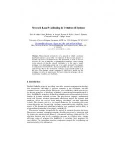
Figure 1.

System Extension

wants to use some data, it accesses the appropriate store, uses the data, and discards it afterwards. For subsequent usage, it must access the store again. Before discarding the data, the agent may write it, possibly after processing it in some way, into the same or a different store. In this way, data can propagate between stores. A consequence of this restriction on the interaction between system entities is that the use of data is always observable at the data stores. Systems are governed by (usage-control) policies, which state requirements on the usage of the data. For example, only agents with particular credentials may modify data, or data must be deleted after two years from a given store. Agents may or may not comply with policies. Logging and Monitoring. Given a system that is an instance of the above system model, we must extend it to support logging and monitoring. To determine whether a policy is violated we usually need to relate actions that are carried out in different parts of the system. Moreover, the ordering of actions and the time elapsed between them is important. To relate actions and the times when they happen, we log them locally, annotating each action with a timestamp, and merge these logs after some pre-processing. We then monitor this merged stream of logged actions. These system extensions are depicted in Figure 1. Challenges and Contributions. Individual logs are totally ordered and timestamped using local clocks. However, even assuming clock synchronization [3], we have only a partial order on system actions [4] as multiple actions with the same timestamp may occur in different logs. Our main theoretical challenge is to monitor such a partially ordered set of actions, which is, in general, an intractable problem. In Section III, we identify a subclass of formulas that describe properties that are insensitive to the ordering of actions labeled by the same timestamp and for which it suffices to monitor a particular merging of the logs, namely, the merging that assumes that actions with equal timestamps happen simultaneously. Furthermore, in case

the given formula is outside this class we provide means to meaningfully monitor this merge by approximating the described property. A practical challenge is to deploy adequate logging mechanisms. The mechanisms should be complete in that they log all occurrences of policy-relevant system actions. They should also be accurate in that if an action is logged then it has happened in the system and the corresponding log entry accurately describes the action, e.g, it describes the involved data and the associated timestamp is the actual time when the action happened. Incomplete or inaccurate logging may lead to false positives and false negatives when monitoring the system. In Section IV, we explain how we handle these practical challenges in our case study. Where possible, we use existing logging mechanisms and extract policy-relevant information from the produced log entries. For system components where no logging was available, we either added logging directly to the components or we extended the components with proxy mechanisms that logged actions. However, proxies have limitations: agents do not necessarily access a store over a proxy and proxies see requested actions but not necessarily all the effects on the involved data. In our case, the interactions could be accurately observed but not for all agents, which led to accurate but incomplete logs. Summarizing, we see our contributions as follows. We provide solutions for efficiently monitoring partially ordered logs, which is a central problem in monitoring real-time concurrent distributed systems. Moreover, we evaluate the performance of our monitoring approach and demonstrate its effectiveness on a real-world application. Organization. The remainder of this paper is structured as follows. In Section II, we give background on MFOTL and our monitor. In Section III, we show how we handle the interleavings of multiple streams of logged actions from different log producers. In Section IV, we report on our case study. In Section V, we discuss related work and in Section VI, we draw conclusions. The Appendices A–D contain additional proof details. Additional details on the case study are given in Appendix E. II. Preliminaries We briefly review metric first-order temporal logic (MFOTL) and describe how we use it to monitor systems. Syntax and Semantics. Let I be the set of nonempty intervals over N. We will write an interval I ∈ I as [b, b0 ) := {a ∈ N | b ≤ a < b0 }, where b ∈ N, b0 ∈ N ∪ {∞}, and b < b0 . A signature S is a tuple (C, R, ι), where C is a finite set of constant symbols, R is a finite set of predicates disjoint from C, and the function ι : R → N associates each predicate r ∈ R with an arity ι(r) ∈ N. In the following, let S = (C, R, ι) be a signature and V a countably infinite set of variables, assuming V ∩ (C ∪ R) = ∅.

¯ τ¯ , v, i) |= t≈ t0 (D, ¯ τ¯ , v, i) |= t≺ t0 (D, ¯ τ¯ , v, i) |= r(t1 , . . . , tι(r) ) (D, ¯ τ¯ , v, i) |= (¬φ) (D, ¯ τ¯ , v, i) |= (φ ∨ ψ) (D, ¯ τ¯ , v, i) |= (∃x. φ) (D, ¯ τ¯ , v, i) |= ( I φ) (D, ¯ τ¯ , v, i) |= (#I φ) (D, ¯ τ¯ , v, i) |= (φ SI ψ) (D, ¯ τ¯ , v, i) |= (φ UI ψ) (D,

v(t) = v(t0 ) v(t) < v(t0 )
v(t1 ), . . . , v(tι(r) ) ∈ rDi ¯ τ¯ , v, i) 6|= φ (D, ¯ τ¯ , v, i) |= φ or (D, ¯ τ¯ , v, i) |= ψ (D, ¯ τ¯ , v[x/d], i) |= φ, for some d ∈ |D| ¯ (D, ¯ τ¯ , v, i − 1) |= φ i > 0, τi − τi−1 ∈ I, and (D, ¯ τ¯ , v, i + 1) |= φ τi+1 − τi ∈ I and (D, ¯ τ¯ , v, j) |= ψ, for some j ≤ i, τi − τ j ∈ I, (D, ¯ τ¯ , v, k) |= φ, for all k ∈ [ j + 1, i + 1) and (D, ¯ τ¯ , v, j) |= ψ, iff for some j ≥ i, τ j − τi ∈ I, (D, ¯ τ¯ , v, k) |= φ, for all k ∈ [i, j) and (D,

iff iff iff iff iff iff iff iff iff

Figure 2.

Semantics of MFOTL

Formulas over the signature S are given by the grammar φ ::= t1≈ t2 t1≺ t2 r(t1 , . . . , tι(r) ) (¬φ) (φ ∨ φ) (∃x. φ) ( I φ) (#I φ) (φ SI φ) (φ UI φ) , where t1 , t2 , . . . range over the elements in V ∪ C, and r, x, and I range over the elements in R, V, and I, respectively. To define MFOTL’s semantics, we need the following notions. A structure D over S consists of a domain |D| , ∅ and interpretations cD ∈ |D| and rD ⊆ |D|ι(r) , for each c ∈ C ¯ τ¯ ), and r ∈ R. A temporal structure over S is a pair (D, ¯ where D = (D0 , D1 , . . . ) is a sequence of structures over S and τ¯ = (τ0 , τ1 , . . . ) is a sequence of natural numbers (i.e., timestamps), where: (1) The sequence τ¯ is monotonically increasing (i.e., τi ≤ τi+1 , for all i ≥ 0) and makes progress (i.e., for every i ≥ 0, there is some j > i such that τ j > τi ). ¯ has constant domains, i.e., |Di | = |Di+1 |, for all i ≥ 0. (2) D ¯ and require that |D| ¯ is We denote the domain by |D| strict linearly ordered by a relation }, such that θ(α) = >, where θ is extended from atomic propositions to formulas as expected. The SAT problem asks whether a given propositional formula is satisfiable. SAT is NP-hard. Suppose P = {p0 , . . . , pn−1 }, with n ≥ 0, is a set of atomic propositions. Let S be the signature (C, R, ι) with C = {c}, R = {q0 , r0 , . . . , qn−1 , rn−1 }, and ι(qi ) = ι(ri ) = 1, for any ¯ 1 , τ¯ 1 ) and (D ¯ 2 , τ¯ 2 ) 0 ≤ i < n. The two temporal structures (D ¯ D 1 2 ¯ over S are given by: |D| = {c}, c = c, τi = τi = i for any i ∈ N, and for any k ∈ {1, 2} and i, j ∈ N with 0 ≤ i < n, ( Dkj {c} if k = 1 and i = j, qi = ∅ otherwise, ( k D {c} if k = 2 and i = j, ri j = ∅ otherwise. Given a propositional formula α over P, the MFOTL formula pαq is obtained by replacing each occurrence of
a proposition pi in α with  ri (c) ∧  qi (c) . Thus, given a propositional formula α, the reduction constructs the two ¯ 1 , τ¯ 1 ) and (D ¯ 2 , τ¯ 2 ) and the MFOTL prefixes of length n of (D formula pαq. This reduction is linear in the size of α. Its correctness is shown by Lemma 13. The following remarks and lemma will be needed. ¯ 2 , τ¯ 2 ), the ¯ τ¯ ) ∈ (D ¯ 1 , τ¯ 1 ) (D Remark. For any interleaving (D, functions f1 and f2 in Definition 1 satisfy fk (i) ∈ {2i, 2i + 1} where k ∈ {1, 2}. Moreover, these functions are unique, ./

[7] I. Aad and V. Niemi, “NRC data collection campaign and the privacy by design principles,” in Proceedings of the International Workshop on Sensing for App Phones (PhoneSense), 2010. [8] A. Pretschner, M. Hilty, and D. Basin, “Distributed usage control,” Commun. ACM, vol. 49, no. 9, pp. 39–44, 2006. [9] J. Park and R. Sandhu, “The UCONABC usage control model,” ACM Trans. Inform. Syst. Secur., vol. 7, no. 1, pp. 128–174, 2004. [10] A. Goodloe and L. Pike, “Monitoring distributed real-time systems: A survey and future directions,” NASA Langley Research Center, Tech. Rep. NASA/CR-2010-216724, July 2010. [11] A. Bauer, M. Leucker, and C. Schallhart, “Model-based runtime analysis of distributed reactive systems,” in Proceedings of the 2006 Australian Software Engineering Conference (ASWEC). IEEE Computer Society, 2006. [12] A. Genon, T. Massart, and C. Meuter, “Monitoring distributed controllers: When an efficient LTL algorithm on sequences is needed to model-check traces,” in Proceedings of the 14th International Symposium on Formal Methods (FM), ser. Lect. Notes Comput. Sci., vol. 4085. Springer, 2006, pp. 557–572. [13] K. Sen, A. Vardhan, G. Agha, and G. Ros¸u, “Efficient decentralized monitoring of safety in distributed systems,” in Proceedings of the 26th International Conference on Software Engineering (ICSE). IEEE Computer Society, 2004, pp. 418– 427. [14] J. Chomicki, “Efficient checking of temporal integrity constraints using bounded history encoding,” ACM Trans. Database Syst., vol. 20, no. 2, pp. 149–186, 1995. [15] U. W. Lipeck and G. Saake, “Monitoring dynamic integrity constraints based on temporal logic,” Inform. Syst., vol. 12, no. 3, pp. 255–269, 1987. [16] A. P. Sistla and O. Wolfson, “Temporal triggers in active databases,” IEEE Trans. Knowl. Data Eng., vol. 7, no. 3, pp. 471–486, 1995. [17] T. Massart, C. Meuter, and L. Van Begin, “On the complexity of partial order trace model checking,” Inform. Process. Lett., vol. 106, no. 3, pp. 120–126, 2008. [18] N. Markey and P. Schnoebelen, “Model checking a path,” in Proceedings of the 14th International Conference on Concurrency Theory (CONCUR), ser. Lect. Notes Comput. Sci., vol. 2761. Springer, 2003, pp. 248–262.

./

Lemma 13. Let α be a propositional formula. It holds that α ¯ 1 , τ¯ 1 ) (D ¯ 2 , τ¯ 2 ) weakly violates is satisfiable if and only if (D ¬pαq at time point 2n. Proof: Suppose first that α is satisfiable. Then there is ¯ τ¯ ) be a truth value assignment θ such that θ(α) = >. Let (D, the interleaving determined by the functions f1 and f2 given by ( 2i if θ(pi ) = >, f1 (i) = 2i + 1 otherwise, and

( f2 (i) =

2i 2i + 1

if θ(pi ) = ⊥, otherwise.

./

Let v be an arbitrary valuation. From Lemma 12, we obtain ¯ τ¯ , v, 2n) |= pαq, that is, (D, ¯ τ¯ , v, 2n) 6|= ¬pαq. that (D, 1 1 ¯ ¯ Suppose now that (D , τ¯ ) (D2 , τ¯ 2 ) weakly violates ¬pαq ¯ τ¯ ) and a at time point 2n. Then there is an interleaving (D, ¯ valuation v such (D, τ¯ , v, 2n) 6|= ¬pαq. Let f1 and f2 the be ¯ τ¯ ) as in Definition 1. Let θ be functions determined by (D, a truth value assignment such that θ(pi ) = > if and only if f1 (i) = 2i. Using again Lemma 12, we get that θ is a satisfying assignment for α.

./

¯ τ¯ ) Proof: Suppose first that α is a tautology. Let (D, 2 2 1 1 ¯ ¯ be an arbitrary interleaving in (D , τ¯ ) (D , τ¯ ) and f1 , f2 be functions as in Definition 1. Let θ be a truth value assignment such that θ(pi ) = > if and only if f1 (i) = 2i. Let v be an arbitrary valuation. Using Lemma 12, we obtain ¯ τ¯ , v, 2n) 6|= ¬pαq. Hence (D ¯ 1 , τ¯ 1 ) (D ¯ 2 , τ¯ 2 ) strongly that (D, violates ¬pαq at time point 2n. ¯ 1 , τ¯ 1 ) (D ¯ 2 , τ¯ 2 ) strongly violates ¬pαq Suppose now that (D at time point 2n. Let θ be an arbitrary truth value assignment. ¯ τ¯ ) be the interleaving determined by the functions Let (D, f1 and f2 given by ( 2i if θ(pi ) = >, f1 (i) = 2i + 1 otherwise, ./

Proof: We use structural induction on the form of α. The only interesting case is the base case, the other cases follow directly from the induction hypotheses. Thus let α = pi ∈ P. ¯ τ¯ , v, 2n) |= (ri (c)∧ qi (c)). That is, there Suppose that (D, ¯ τ¯ , v, j) |= ri (c) and such is a time point j ≤ 2n such that (D, ¯ τ¯ , v, j0 ) |= that there is a time point j0 ≤ j for which (D, D j0 Dj qi (c). Then c ∈ ri and c ∈ qi . From the definition of an interleaving and the definitions of the interpretations of the predicates qi and ri , it follows that j = f2 (i) and j0 = f1 (i). Then, as f1 (i), f2 (i) ∈ {2i, 2i + 1}, f1 (i) , f2 (i), and j0 ≤ j, we get that f1 (i) = 2i and f2 (i) = 2i + 1. Thus θ(pi ) = >. Suppose that θ(α) = >. Then f1 (i) = 2i and f2 (i) = 2i + 1. ¯ τ¯ , v, 2i) |= qi (c) and (D, ¯ τ¯ , v, 2i+1) |= ri (c). Thus We have (D, ¯ ¯ τ¯ , v, 2n) |= (D, τ¯ , v, 2i + 1) |= ri (c) ∧  qi (c) and clearly (D,
 ri (c) ∧  qi (c) .

Lemma 14. Let α be a propositional formula. It holds that ¯ 2 , τ¯ 2 ) strongly ¯ 1 , τ¯ 1 ) (D α is a tautology if and only if (D violates ¬pαq at time point 2n.

./

./

Lemma 12. Let α be a propositional formula, θ a truth ¯ τ¯ ) an interleaving value assignment, v a valuation, and (D, 2 2 1 1 ¯ ¯ of (D , τ¯ ) (D , τ¯ ) given by the functions f1 and f2 such that θ(pi ) = > iff f1 (i) = 2i, for any i with 0 ≤ i < n. It holds ¯ τ¯ , v, 2n) |= pαq. that θ(α) = > if and only if (D,

Reduction from TAUT. We show coNP-hardness of the decision problem in Theorem 3(2) by reduction from TAUT. We recall that a propositional formula α over a set of atomic propositions P is a tautology if θ(α) = > for any assignment θ of propositions to truth values. The TAUT problem asks whether a given propositional formula is a tautology. TAUT is coNP-hard. We use the same reduction as for the decision problem in Theorem 3(1). The correctness of the reduction follows from the following lemma.

./

that is, if g1 , g2 : N → N are strictly monotonic functions satisfying conditions (1)–(3) in Definition 1 then either g1 = f1 and g2 = f2 , or g1 = f2 and g2 = f1 . Furthermore, for any strictly monotonic functions f1 and f2 satisfying conditions (1) and (2) in Definition 1 and with f1 (i), f2 (i) ∈ {2i, 2i + 1} ¯ τ¯ ) for 0 ≤ i < n, there is a unique temporal structure (D, such that f1 and f2 also satisfy condition (3). In other words, ¯ 1 , τ¯ 1 ) and the functions f1 , f2 determine an interleaving of (D ¯ 2 , τ¯ 2 ) (D

and ( f2 (i) =

2i 2i + 1

if θ(pi ) = ⊥, otherwise.

¯ τ¯ , v, 2n) 6|= ¬pαq. Using again There is a valuation v such (D, Lemma 12, we get that θ is a satisfying assignment for α. Hence α is a tautology. B. Additional Proof Details: Derivation Rules Figure 5 lists all the inference rules for label propagation. Lemma 15 (see below) shows the soundness of these rules. When considering formulas in positive normal form, as required in Theorem 11, the Boolean operator ∨ and the temporal operators release RI and trigger TI are seen as primitives, instead of being defined as syntactic sugar. We recall that ψ RI χ abbreviates ¬(¬ψ SI ¬χ) and ψ TI χ abbreviates ¬(¬ψ UI ¬χ). Figure 6 lists propagation rules for formulas that use these operators. Their soundness follows from the soundness of rules in Figure 5 and the mentioned equivalences. For instance, the correctness of the rule ψ : (|= ∃) χ : (|= ∀) 0 < I, 0 ∈ J (ψ RI χ) ∨ (♦ J ψ) : (|= ∀) follows from unfolding the abbreviation (ψ RI χ) ∨ (♦ J ψ),
which is ¬ (¬ψ SI ¬χ) ∧ ( J ¬ψ) , and the following deriva-

tion:

•

ψ : (|= ∃) χ : (|= ∀) ¬ψ : (6|= ∃) ¬χ : (6|= ∀) 0 < I, 0 ∈ J (¬ψ SI ¬χ) ∧ ( J ¬ψ) : (6|= ∀)
¬ (¬ψ SI ¬χ) ∧ ( J ¬ψ) : (|= ∀)

•

Finally, for convenience, Figure 7 lists some inference rules for formulas for which the main operator is one of the temporal operators I , ♦I , I , and I . These rules can be derived from the rules in Figure 5 by simply applying the definition of syntactic sugar. For instance, the rule ψ : (|= ∀) I ψ : (|= ∀)

•

can be derived from x ≈ x : (|= ∀) ∃x. x ≈ x : (|= ∀) ψ : (|= ∀) (∃x. x ≈ x) SI ψ : (|= ∀) Note that I ψ is syntactic sugar for (∃x. x ≈ x) SI ψ. We now show the soundness of the inference rules in Figure 5.

•

Lemma 15. Let φ be a formula. If φ can be labeled with `, then φ satisfies the invariant `, where ` ∈  (|= ∀), (6|= ∀), (6|= ∃), (|= ∃) . ¯ κ¯ ) be the collapse of an interleaving of Proof: Let (C, two given temporal structures. We proceed by induction on size of the derivation tree assigning label ` to φ. We make a case distinction based on the rule applied to label the formula, that is, the rule at the root of the tree. However, for clarity, we generally group cases by the formula’s form. For readability, and without loss of generality, we already fix an arbitrary valuation v, an arbitrary time point i, and an ¯ τ¯ ) ∈ col−1 (C, ¯ κ¯ ). arbitrary temporal structure (D, • We first consider the weakening rules. – φ is labeled with (|= ∀) and (|= ∃). Suppose that ¯ κ¯ , v, i) |= φ. By the induction hypothesis, φ sat(C, ¯ τ¯ , v, j) |= φ for any isfies the invariant (|= ∀), thus (D, ¯ κ¯ ), there is j with τ j = κi . By the definition of (C, at least one j with τ j = κi . Hence φ satisfies the invariant (|= ∃). – φ is labeled with (6|= ∀) and with (6|= ∃). This case is analogous to the previous one. 0 0 • φ = t ≈ t , where t and t are variables or constants. In this case φ is labeled with (|= ∀) and (6|= ∀). ¯ κ¯ , v, i) |= φ. – φ is labeled with (|= ∀). Suppose that (C, ¯ τ¯ , v, j) |= φ for any Then v(t) = v(t0 ). Clearly, (D, time point j, as φ only depends on the valuation. The invariant (|= ∀) is hence satisfied. – φ is labeled with (6|= ∀). This case is analogous to the previous one.

•

•

φ = t ≺ t0 , where t and t0 are variables or constants. This case is analogous to the previous one. φ = r(t1 , . . . , tι(r) ), where t1 , . . . , tι(r) are variables or constants. In this case φ is labeled with (|= ∃) and (6|= ∀). ¯ κ¯ , v, i) |= φ. – φ is labeled with (|= ∃). Suppose that (C, S Then (v(t1 ), . . . , v(tι(r) )) ∈ rCi . As rCi = { j|τ j =κi } rD j , there is a j with τ j = κi such that (v(t1 ), . . . , v(tι(r) )) ∈ ¯ τ¯ , v, j) |= φ. Thus φ satisfies the rD j . Therefore (D, invariant (|= ∃). ¯ κ¯ , v, i) 6|= – φ is labeled with (6|= ∀). Suppose that (C, φ. Then for any j with τ j = κi we have that ¯ τ¯ , v, j) |= φ. Thus (v(t1 ), . . . , v(tι(r) )) < rD j , that is, (D, φ satisfies the invariant (6|= ∀). φ = ¬ψ. If ψ is labeled with `, then φ is labeled with ¬`, where ¬` is (|= ∀), (6|= ∀), (6|= ∃), or (|= ∃) when ` is (6|= ∀), (|= ∀), (|= ∃), or (6|= ∃) respectively. ¯ κ¯ , v, i) |= – φ is labeled with (|= ∀). Suppose that (C, ¬ψ. By the induction hypothesis, ψ satisfies the ¯ κ¯ , v, i) 6|= ψ, we have that invariant (6|= ∀). As (C, ¯ τ¯ , v, k) 6|= ψ, that is, (D, ¯ τ¯ , v, k) |= φ, for all k (D, with τk = κi . Thus φ satisfies the invariant (|= ∀). – The other cases are similar. φ = ψ ∧ χ. There are four rules to be analyzed. – φ, ψ, and χ are labeled with (|= ∀). Suppose that ¯ κ¯ , v, i) |= ψ ∧ χ. Then (C, ¯ κ¯ , v, i) |= ψ and (C, ¯ κ¯ , v, i) |= χ. By the induction hypothesis, ψ and (C, χ satisfy the invariant (|= ∀). Hence, for all j with ¯ τ¯ , v, j) |= ψ and (D, ¯ τ¯ , v, j) |= χ. τ j = κi , we have (D, ¯ τ¯ , v, j) |= φ and (D, ¯ τ¯ , v, j) |= χ for all j Thus (D, with τ j = κi . Hence, φ satisfies the invariant (|= ∀). – The other cases are similar. φ = ∃x.ψ. There are four rules, one for each label: if ψ is labeled with `, then φ is labeled with `. ¯ κ¯ , v, i) |= ∃x.ψ. Then there – ` is (|= ∀). Suppose that (C, ¯ ¯ is a d ∈ |D| such that (C, κ¯ , v[x/d], i) |= ψ. As ψ satis¯ τ¯ , v[x/d], j) |= ψ fies the invariant (|= ∀), we have (D, ¯ τ¯ , v, j) |= ∃x.ψ for all j with τ j = κi . That is, (D, for all j with τ j = κi . Hence φ satisfies the invariant (|= ∀). – The other cases are similar. φ = ψ SI χ. We have three rules to analyze. – φ, ψ, and χ are each labeled with (|= ∀). By the induction hypothesis, ψ and χ satisfy the invariant ¯ κ¯ , v, i) |= φ. Then, for some (|= ∀). Suppose that (C, ¯ κ¯ , v, j) |= χ and j ≤ i with κi − κ j ∈ I, we have (C, ¯ (C, κ¯ , v, k) |= ψ for all k ∈ [ j + 1, i + 1). Let i0 be an arbitrary time point such that τi0 = κi . As χ satisfies the invariant (|= ∀), for the largest j0 with τ j0 = κ j we ¯ τ¯ , v, j0 ) |= χ. Clearly, τi0 − τ j0 ∈ I. From the have (D, ¯ κ¯ ), for any k0 ∈ [ j0 + 1, i0 + 1), there definition of (C, is a k ∈ [ j + 1, i + 1) such that τk0 = κk . Then, as ψ satisfies the invariant (|= ∀), for any k0 ∈ [ j0 +1, i0 +1), ¯ τ¯ , v, k0 ) |= ψ. As ψ satisfies the invariant we have (D, (|= ∀), for all k ∈ [ j + 1, i + 1) and all k0 with τk0 = κk ,

φ : (|= ∀) φ : (|= ∃) t ≈ t0 : (|= ∀)

t ≈ t0 : (6|= ∀)

r(t1 , . . . , tι(r) ) : (|= ∃) ψ : (|= ∃) ¬ψ : (6|= ∃)

ψ : (|= ∀) ¬ψ : (6|= ∀)

φ : (6|= ∀) φ : (6|= ∃) t ≺ t0 : (|= ∀)

t ≺ t0 : (6|= ∀)

r(t1 , . . . , tι(r) ) : (6|= ∀) ψ : (6|= ∃) ¬ψ : (|= ∃)

ψ : (6|= ∀) ¬ψ : (|= ∀)

ψ : (|= ∀) χ : (|= ∀) ψ ∧ χ : (|= ∀)

ψ : (|= ∀) χ : (|= ∃) ψ ∧ χ : (|= ∃)

ψ : (6|= ∀) χ : (6|= ∀) ψ ∧ χ : (6|= ∀)

ψ : (6|= ∃) χ : (6|= ∃) ψ ∧ χ : (6|= ∃)

ψ : (|= ∀) ∃x. ψ : (|= ∀)

ψ : (|= ∃) ∃x. ψ : (|= ∃)

ψ : (6|= ∀) ∃x. ψ : (6|= ∀)

ψ : (6|= ∃) ∃x. ψ : (6|= ∃)

ψ : (|= ∀) χ : (|= ∀) ψ SI χ : (|= ∀)

ψ : (6|= ∀) χ : (6|= ∀) ψ SI χ : (6|= ∀)

ψ : (6|= ∃) χ : (6|= ∀) ψ SI χ : (6|= ∃)

ψ : (6|= ∃) χ : (6|= ∀) 0 < I, 0 ∈ J (ψ SI χ) ∧ ( J ψ) : (6|= ∀)

ψ : (|= ∀) χ : (|= ∀) ψ UI χ : (|= ∀)

ψ : (6|= ∀) χ : (6|= ∀) ψ UI χ : (6|= ∀)

ψ : (6|= ∃) χ : (6|= ∀) ψ UI χ : (6|= ∃)

ψ : (6|= ∃) χ : (6|= ∀) 0 < I, 0 ∈ J (ψ UI χ) ∧ ( J ψ) : (6|= ∀)

ψ : (|= ∃) I ψ : (|= ∃)

ψ : (|= ∃) 0