Euclidean distance between points i and j (dij = qi â qj ) x. True value of x (for x = qi ... These ideas have been implemented in different manners. For instance, [3].
Monocular Template-based Reconstruction of Smooth and Inextensible Surfaces F. Brunet1,2 , R. Hartley3 , A. Bartoli1 , N. Navab2 , and R. Malgouyres4 1
ISIT, Universit´e d’Auvergne, Clermont-Ferrand, France CAMPAR, Technische Universt¨ at M¨ unchen, Germany Research School of Information Sciences, ANU, NICTA, Australia 4 LIMOS, UMR 6158, Clermont-Ferrand, France 2
3
Abstract. We present different approaches to reconstructing an inextensible surface from point correspondences between an input image and a template image representing a flat reference shape from a frontoparallel point of view. We first propose a ‘point-wise’ method, i.e. a method that only retrieves the 3D positions of the point correspondences. This method is formulated as a second-order cone program and it handles inaccuracies in the point measurements. It relies on the fact that the Euclidean distance between two 3D points must be shorter than their geodesic distance (which can easily be computed from the template image). We then present an approach that reconstructs a smooth 3D surface based on Free-Form Deformations. The surface is represented as a smooth map from the template image space to the 3D space. Our idea is to say that the 2D-3D map must be everywhere a local isometry. This induces conditions on the Jacobian matrix of the map which are included in a least-squares minimization problem.
1
Introduction
Monocular surface reconstruction of deformable objects is a challenging problem which has known renewed interest during the past few years. This problem is fundamentally ill-posed because of the depth ambiguities; there are virtually an infinite number of 3D surfaces that have exactly the same projection. It is thus necessary to use additional constraints ensuring the consistency of the reconstructed surface. In this paper, we present two algorithms for monocular reconstruction of deformable and inextensible surfaces under some general assumptions. First, we consider the template-based case. Reconstruction is achieved from point correspondences between an input image and a template image showing a flat reference shape from a fronto-parallel point of view. Second, we suppose the intrinsic parameters of the camera to be known. Third, we assume that the camera is a perspective camera. These are common assumptions [1–3]. Over the years, different types of constraints have been proposed to disambiguate the problem of monocular reconstruction of deformable surfaces.
2
F. Brunet et al.
They can be divided into two main categories: the statistical and the physical constraints. For instance, the methods relying on the low-rank factorization paradigm [4–10] can be classified as statistical approaches. Learning approaches such as [11–13, 1] also belong to the statistical approaches. Work such as [1], where the reconstructed surface is represented as a linear combination of inextensible deformation modes, is also a statistical approach. Physical constraints include spatial and temporal priors on the surface to reconstruct [14, 15]. Statistical and physical priors can be combined [5, 7]. A physical prior of particular interest is the hypothesis of having an inextensible surface [16, 2, 1, 3]. In this paper, we consider this type of surface. This hypothesis means that the geodesics on the surface may not change their length across time. However, computing geodesics is generally hard to achieve and it is even more difficult to incorporate such constraints in a reconstruction algorithm. There exist several approaches to approximate this type of constraint. For instance, if the points are sufficiently close together, the geodesic between two 3D points on the surface can be approximated by the Euclidean distance [17]. An efficient approximation consists in saying that the geodesic distance between two points is an upper bound to the Euclidean distance [16, 3]. Algorithms for monocular reconstruction of deformable surfaces can also be categorized according to the type of surface model (or representation) they use. The point-wise methods utilize a sparse representation of the 3D surface, i.e. they only retrieve the 3D positions of the data points [3]. Other methods use more complex surface models such as triangular meshes [16, 1] or smooth surfaces such as Thin-Plate Splines [3, 5]. In this latter case, the 3D surface is represented as a parametric 2D-3D map between the template image space and the 3D space. Smooth surfaces are generally obtained by fitting a parametric model to a sparse set of reconstructed 3D points: the smooth surface is not actually used in the 3D reconstruction process. In this paper, we propose an algorithm that directly estimates a smooth 3D surface based on Free-Form Deformations [18]. Having an inextensible surface means that the surface must be everywhere a local isometry. This induces conditions on the Jacobian matrix of the 2D-3D map. We show that these conditions can be integrated in a non-linear least-squares minimization problem along with some other constraints that force the consistency between the reconstructed surface and the point correspondences. Such a problem can be solved using an iterative optimization procedure such as Levenberg-Marquardt that we initialize using a point-wise reconstruction algorithm. Our approach is highly effective in the sense that it outperforms previous approaches in terms of accuracy of the reconstructed surface and in terms of inextensibility. Another important aspect in monocular reconstruction of deformable surfaces is the way noise is handled. It can be accounted for in the template image [3] or in the input image [1]. There exist different approaches for handling the noise. For instance, one can minimize a reprojection error, i.e. the distance between the data points of the input image and the projection of the reconstructed 3D points. It is also possible to hypothesize maximal inaccuracies in the data points. We propose a point-wise approach that accounts for noise in both the template and
Reconstruction of Inextensible Surfaces
3
the input images. This approach is formulated as a second-order cone program (SOCP) [19].
Notation Description P Matrix of the intrinsic parameters of the camera (P ∈ R3×3 ) (The camera is assumed to be at the coordinate origin, so the matrix P may be assumed to be square and invertible.)
pTk nc qi q0i ¯i q ui µi Qi dij x ˆ
2
kth row of the matrix P Number of point correspondences ith point in the template image ith point in the input image; i ∈ {1, . . . , nc } Point qi in homogeneous coordinates ¯ 0i )/kP−1 q ¯ 0i k) Sightline corresponding to the point q0i (ui = (P−1 q Depth of the point Qi Reconstructed 3D point i Euclidean distance between points i and j (dij = kqi − qj k) True value of x (for x = q0i , qi , Qi , ui , µi , dij ) Table 1. Notation used in this paper.
Related Work on Inextensible Surface Reconstruction
A popular assumption made in deformable surface reconstruction is to consider that the surface to reconstruct is inextensible [16, 2, 1, 3]. This assumption is reasonable for many types of material such as paper and some types of fabrics. Having an inextensible surface means that the surface is an isometric deformation of the reference shape. Another way of putting it is to say that the length of the geodesics between pairs of points remains unchanged when the surface deforms. An exact transcription of this principle is difficult to integrate in a reconstruction algorithm. Indeed, while it is trivial to compute the geodesic in a flat reference shape, it is quite difficult to do it for a bent surface (especially when the surface is represented as a sparse set of points or a triangular mesh). Many approximations have thus been proposed. The first type of approximation consists in saying that if the surface does not deform too much then the Euclidean distance is a good approximation to the geodesic distance. Such an approach has been used for instance in [12, 16, 20, 2]. Note that these types of constraints are usually set in a soft way. For a given set of point pairs on the surface, the Euclidean distance should not diverge too much from the geodesic distances. This approximation is better when there are a large number of points. Depending on the surface model it is not always possible to vary the number of points. Although the Euclidean approximation can work well in some cases, this approximation gives poor results when creases appear in the 3D surface. In this case, the Euclidean distance between two points on the surface can shrink, as
4
F. Brunet et al.
illustrated in figure 1. The ‘upper bound approach’ is a now classical approach [1,
Fig. 1. Inextensible object deformation. The Euclidean distance between two points is necessarily less than or equal to the length of the geodesic that links those two points (this length is easily computable if we have a template image representing the flat reference surface from a fronto-parallel point of view).
3] which consists in noticing that even if the Euclidean distance between two points can shrink it can never be greater than the length of the corresponding geodesic. In other words, the inextensibility constraint kQi − Qj k ≤ dij must be satisfied for any pair of points (Qi , Qj ) lying on the surface. The second principle of such algorithms is to say that a 3D point Qi must lie on the sightline ui , i.e. Qi = µi ui . These two constraints are not sufficient to reconstruct the surface. Indeed, nothing prevents the reconstructed surface from shrinking towards the optical centre of the camera. This problem is ‘solved’ using a heuristic that has been proven to be very effective in practice. It consists in considering a perspective camera and in maximizing the depth of the reconstructed 3D points. These ideas have been implemented in different manners. For instance, [3] proposes a dedicated algorithm that enforces the inextensibility constraints. This algorithm accounts for noise only in the template image (by simply increasing a little bit the geodesic distances in the template, i.e. by replacing dij with dij +εT where εT is the maximal inaccuracy of the points in the template image). Another sort of implementation is given by [16, 1]. In these papers, a convex cost function combining the depth of the reconstructed points and the negative of the reprojection error is maximized while enforcing the inequality constraints arising from the surface inextensibility. The resulting formulation can be easily turned into an SOCP problem. A similar approach is explored in [2]. These last two methods account for noise in the input image. The approach of [3] is a pointwise method. The approaches of [16, 1, 2] use a triangular mesh as surface model, and the inextensibility constraints are applied to the vertices of the mesh.
3
Convex Formulation of the Upper Bound Approach with Noise in all Images
In this section, we propose a convex formulation of the principles sketched in §2 that, compared to [3], accounts for noise in both the template and the input
Reconstruction of Inextensible Surfaces
5
images. We can express this in terms of image-plane measurements. As in [16, 1], our approach is formulated as an SOCP problem. However, contrary to [16, 1], our approach is a point-wise method that does not require us to tune the relative influence of minimizing the reprojection error and maximizing the depths. 3.1
Noise in the Template Only
Let us first remark that the basic principles explained in §2 can be formulated as SOCP problems. In this first formulation, the noise is only account for in the template image. The inextensibility constraint kQi − Qj k ≤ dij + εT can be written: kµi ui − µj uj k ≤ dij + εT . (1) Including the maximization of the depths, we obtain this SOCP problem: max µ
nc X
µi
i=1
subject to kµi ui − µj uj k ≤ dij + εT
∀(i, j) ∈ E
(2)
µi ≥ 0 i ∈ {1, . . . , nc } � where µT = µ1 . . . µnc , and E is a set of pairs of points to which the inextensibility constraints are applied. 3.2
Noise in Both the Template and the Input Images
Let us now suppose that the inaccuracies are expressed in terms of image-plane measurements. Suppose that points are measured in the image with a maximum error of εI , i.e. kˆ q0i − q0i k ≤ εI , ∀i ∈ {1, . . . , nc }. (3) Since we are searching for the true 3D position of the point Qi , we say that: � T � 1 p1 Qi ˆ 0i = T . (4) q p3 Qi pT 2 Qi Equation (3) can thus be rewritten:
� T �
1 p1 Qi 0
− q i ≤ εI .
pT Q pT 2 Qi 3 i
(5)
We finally add the inextensibility constraints and the maximization of the depths (which are given by pT 3 Qi ) and we obtain the following SOCP problem: max pT 3 Q
subject to
nc X
Qi i=1
� T �
p1
T Qi
p2
T
− q0i pT Q 3 i ≤ εI p3 Qi ∀i ∈ {1, . . . , nc }
kQi − Qj k ≤ dij
∀(i, j) ∈ E
pT 3 Qi ≥ 0
∀i ∈ {1, . . . , nc }
(6)
6
F. Brunet et al.
where Q is the concatenation of the 3D points Qi , for i ∈ {1, . . . , nc }.
4
Smooth and Inextensible Surface Reconstruction
Pnc µi described in Although the strategem of maximizing the sum of depths i=1 the previous section gives reasonable results, it is merely a heuristic, not based on any valid principle related to surface properties. We therefore consider next a new formulation based on the principle of surface inextensibility. Let the surface be modelled as a function W : R2 → R3 , mapping the planar template to 3-dimensional space. The inextensibility constraint is equivalent to saying that the map W must be everywhere a local isometry. This condition may be expressed in terms of its Jacobian. Let J(q) ∈ R3×2 be the Jacobian matrix ∂W/∂q evaluated at the point q. The map W is an isometry at q if the columns of J(q) are orthonormal. This local isometry can be enforced for the whole surface with the following least-squares constraint: ZZ
J(q)T J(q) − I2 2 dq = 0. (7) In practice, we consider a discretization of the quantity in equation (7), namely Ei (W) =
nj X
J(gj )T J(gj ) − I2 2 ,
(8)
j=1 n
j where {gj }j=1 is a set of 2D points in the template image space taken on a fine and regular grid (for instance, a grid of size 30 × 30). This term Ei (W) measures the departure from inextensibility of the surface W. Our minimization problem is then to minimize this quantity, over all possible surfaces, subject to the projection constraints, namely that point W(qi ) projects to (or near to) the image point q0i , for all i.
4.1
Parametric Surface Model
The problem just described involves a minimization over all possible surfaces. Instead of considering this as a variational problem over all possible surfaces, we consider a parametrized family of surfaces. For this purpose, we chose FreeForm Deformations (FFD) [18] based on uniform cubic B-splines [21]. Let W` : R2 → R3 be the parametric FFD, parametrized by a family of 3D points `jk ; j ∈ {1, . . . , nu }, k ∈ {1, . . . , nv }, which act as ‘attractors’ for the surface. For a point q = (u, v) in the template, the surface point is explicitly given as W` (q) =
nu X nv X
`jk Nj (u)Nk (v).
(9)
j=1 k=1
The functions Nj are the B-spline basis functions [21] which are polynomials of degree 3. If point qi = (ui , vi ) is fixed and known then the surface point W` (qi )
Reconstruction of Inextensible Surfaces
7
is expressed as a linear combination of the points `jk , and hence can be written in the form W` (qi ) = Wi `, where Wi is a 3×nu nv matrix depending only on the point qi , and ` is the vector obtained by concatenating all the points `jk . Thus, the 3D point is a linear expression in terms of the parameter vector `. Since the polynomials Nj and Nk depend only on a local set of the attractor points `jk , the matrix Wi is sparse, which is important for computational efficiency. 4.2
Surface Reconstruction as a Least-Squares Problem
By replacing Qi by Wi ` in (6) we may arrive at a constraint:
�� T � �
p1 T 0 T
− q p W ` i ≤ εI p3 Wi `. i 3
pT 2
(10)
We may then formulate the optimization problem as minimizing the inextensibility cost Ei (W` ) given in (8) over all choices of parameters `, subject to constraints (10). The constraints are SOCP constraints, but the cost function (8) is of higher degree in the parameters. To avoid the difficulties of constrained non-linear optimization, we choose a different course, by including the reprojection error into the cost function, leading to an unconstrained problem. To simplify the formulation of the reprojection error, we introduce the depths µi as subsidiary variables, for reasons that become evident below. This is not strictly necessary, but reduces the degree of the reprojection-error term. The minimization problem now takes the form: min Ed (µ, `) + αEi (`) + βEs (`), µ,`
(11)
where Ed , Ei , Es are the data (reprojection error), inextensibilty, and smoothing terms respectively. The data term ensures the consistency of the point correspondences with the reconstructed surface. Ei forces the inextensibility of the surface. Es promotes smooth surface in order to cope with, for instance, lack of data. The relative influence of these three terms are controlled with the weights α ∈ R+ and β ∈ R+ . The inextensibility term has been described previously. We now describe the two other terms in (11). Data term. Replacing Qi by Wi ` in (5) gives an expression for the reprojection error associated with some point. However, the resulting expression is non-linear with respect to the parameters `. We thus prefer a linear data term expressed in terms of ‘3D errors’, which is the reason why we introduced the depths µ of the data points in the optimization problem. The data term is then defined by: Ed (µ, `) =
nc X
2
W (qi ) − µi P−1 q ¯ 0i , `
(12)
i=1
which measures the distance between the point W` on the surface and the point at depth µi along the ray defined by q0i .
8
F. Brunet et al.
Smoothing term. In some cases, the point correspondences and the hypothesis of an inextensible surface are not sufficient. For instance, imagine that there is no point correspondence in a corner of the surface. In this case, there is nothing that indicates how the surface should behave. The corners of the surface can bend freely as long as they do not extend or shrink (like the corners of a piece of paper). To overcome this difficulty, we can add a third term (the smoothing term) in our cost function that favours non-bending surfaces. Note that usually, such terms are used to compensate for the undesirable effects of under-fitting and over-fitting. Doing so is usually a problem because it requires one to determine a correct value for the weight associated to the smoothing term (value β in equation (11)). This is a sensible and critical way of balancing the effective complexity of the surface against the complexity of the data. Here, we do not have to care too much. Indeed, the complexity of the surface is limited by the fact that it is inextensible. Any small value (but big enough to be not negligible, for instance β = 10−4 ) is thus suitable for the weight of the smoothing term. We define our smoothing term using the bending energy:
2
3 ZZ 2 i
X
∂ W` (q) Es (µ, `) =
dq.
∂q2 i=1
(13)
F
where W`i (q) is the i-th coordinate of the point, and k · kF is the Frobenius norm of the Hessian matrix. With FFD, there exists a simple and linear closed-form expression for the bending energy: Es (`) = kB1/2 `k2 = `T B`
(14)
where B ∈ R3p×3p is a symmetric, positive, and semi-definite matrix which can be easily computed from the second derivatives of the B-spline basis functions.
Initial solution. The problem of equation (11) is a non-linear least-squares minimization problem typically solved using an iterative scheme such as LevenbergMarquardt. Such an algorithm requires a correct initial solution. We used an FFD surface fitted to the 3D points reconstructed with one of the point-wise methods presented in §3. Subsequently, since we use a surface model which is linear with respect to its parameters, the initial parameters ` can be found by solving the least-squares problem: nc nc X X
2
W (qi ) − Qi 2 ⇔ min min kWi ` − Qi k . ` ` i=1 ` i=1
(15)
An alternative is to modify the problem (6), expressing Qi in terms of the required parameters `, according to Qi = Wi `. Then one may solve for ` directly using SOCP. If necessary, the linear smoothing term of equation (13) can be included in equation (15).
Reconstruction of Inextensible Surfaces
5 5.1
9
Experimental Results Experiments on Synthetic Data
In this section, we experiment several aspects of different reconstruction algorithms. We first use synthetic piece of papers, such as those of figure 2, randomly generated using the code provided by [22]. The piece of papers are square and 200mm wide. The input images are simulated by projecting the deformed piece of paper with a virtual camera placed at approximately 1 meter of the paper sheet and with a focal length of 36mm. A set of nc point correspondences are generated by taking random locations on the 3D surface. A zero mean Gaussian noise with standard deviation of 1 pixel is added to the point correspondences. There are no self-occlusion in the data.
Fig. 2. Example of randomly generated piece of paper. Left: 3D surface. Middle: template image. Right: input image. The blue dots are examples of point correspondences.
Several algorithms are compared in our experiments: – SOCPimg: our point-wise method described in §3.2 ; – FFDref: our smooth reconstruction algorithm described in §4.2 ; – FFDinit: the initial solution of our smooth reconstruction algorithm, as described in §4.2 ; – Salz: the convex formulation proposed in [1]. This method is similar to SOCPimg except for the noise that is not handled the same way. In [1], the author minimizes a cost function that includes a ‘reprojection error’ in order to cope with the noise. In SOCPimg, the noise is handled with hard constraints. – PerrioInit: the ‘upper depth bound’ approach of [23, 3] which is a point-wise algorithm that iteratively enforces the inextensibility constraints ; – PerrioRef: the ‘refined approach’ of [23, 3] which minimizes a cost function resulting in a refined estimation of the 3D points obtained with PerrioInit. Reconstruction Errors. The discrepancy between the reconstructed and the ground truth surfaces are quantified with two measures, depending on the surface model used by the algorithms. The point-wise reconstruction error (pwre), denoted ep , can be used for all the algorithms. It is defined by: ep =
nc 1 X ˆ i k. kQi − Q nc i=1
(16)
10
F. Brunet et al.
For algorithms that uses more complex surface models, such as triangular meshes or FFD, we measure the surface reconstruction error (sre), denoted es . It is the ˆ difference between the reconstructed surface W` and the ground truth surface W: ZZ
ˆ
W (q) − W(q)
dq. es = (17) ` In this experiment, we use 1,000 randomly generated paper sheets with 150 points correspondences. Figure 3(a) shows the pwre for all the algorithms and figure 3(b) shows the sre for the algorithms that use a complex surface model. The main result of this experiment is that our approach FFDref gives the smallest reconstruction errors (pwre and sre). Globally, the methods that use complex surface models get better results than the point-wise approaches.
2 1 0.5
2 1 0.5
FF
(a) Point-wise reconstruction error
f re D FF
Sa
D in it
lz
re D
in
FF
FF
D
ef
t ni
oR
rri Pe
Pe
rri
oI
Sa
Pi m SO C
f
10 5
it
10 5
lz
100 50
g
100 50
(b) Surface reconstruction error
Fig. 3. Comparison of the reconstruction errors for different algorithms. The central red line is the median. The limits of the blue box are the 25th and the 75th percentiles. The black ‘whiskers’ cover approximately 99.3% of the experiment outcomes. The green crosses are the maximal errors over the 1000 trials.
Length of Geodesics. When a reconstructed 3D surface is reconstructed in a truly inextensible way, the transformation of the straight line linking two points in the template image must be the geodesic linking the corresponding two 3D points on the surface. In particular, the length of these two paths must be identical. Testing this hypothesis for our algorithms FFDinit and FFDref is the goal of this experiment. To do so, we use the same data as in the previous experiment. For each surface, we choose randomly 10,000 pairs of points in the template im3D age. For each pair of points (gi , gj ), the length lij of the deformed path linking the 3D points W` (gi ) and W` (gj ) on the surface is approximated by the length of the polygonal line linking these two points with the following formula: 3D lij
ng X
=
W` gi +
k ng kgj
� − gi k − W` gi +
k−1 ng kgj
�
− gi k ,
(18)
k=1
where ng is the number of intermediate points used for the approximation (we use ng = 200 since we experimentally observed that the approximation stabilizes for values of ng greater than 180). The lengths of the deformed paths are plotted
Reconstruction of Inextensible Surfaces
11
against their reference length in the template image in figure 4(a) for FFDinit and in figures 4(b,c) for FFDref. Figures 4(b) and 4(c) show that, with the surfaces reconstructed with FFDref, the length of the deformed paths are almost equal to the length they should have if they were actual geodesics. In other words, our approach FFDref reconstructs 3D surfaces which are truly inextensible. On the other hand, figure 4(a) shows that the initial solution FFDinit (which is just an FFD fitted to a sparse set of reconstructed 3D points) seems to be much less inextensible.
(a) FFDinit
(b) FFDref
(c) Magnification of (b)
Fig. 4. Plot of the length of deformed paths against the length they should have if the reconstructed surface was truly inextensible. The red diagonal line is the place where all the blue points should be for inextensible surfaces.
2D Let lij be the Euclidean distance between the points gi and gj . Table 2 gives 3D some statistics on the relative error between the computed length lij and the 2D 2D 2D 3D reference length lij , i.e. the quantity (lij − lij )/lij . These numbers confirm the results seen in figure 4.
Mean Std deviation Median Minimum Maximum FFDinit 0.0119 0.0417 0.0036 −1.9689 0.8931 FFDref 2.0084 × 10⁻⁵ 7.1965 × 10⁻⁴ 5.8083 × 10⁻⁶ −0.0505 0.3396 Table 2. Statistics on the relative errors between the length of transformed paths and the length they should have.
Gaussian curvature. The Gaussian curvature is the product of the two principal curvature (which are the reciprocal of the radius of the osculating circle). For an inextensible surface, the Gaussian curvature is null. In this experiment, we check if this property is satisfied by the smooth surfaces reconstructed with FFDinit and FFDref. We used the same 1,000 reconstructed surfaces as in the previous experiment. The Gaussian curvature, denoted κ, is computed for 10,000 randomly chosen points on the surface with the formula κ = det(II) det(I) , where I and II are the first and the second fundamental forms of the parametric surface [24]. The results of this experiment are reported in table 3. It shows that, in average, the Gaussian curvature of the surfaces reconstructed using FFDref
12
F. Brunet et al.
are consistently close to 0. It also shows that FFDref gives Gaussian curvatures which are 100 times smaller than the ones obtained with FFDinit. These results demonstrate that the surfaces reconstructed with our approach FFDref are indeed inextensible. Note that this kind of experiment cannot be achieved if a smooth surface is not available. Mean Std deviation Median Minimum Maximum −4 −5 FFDinit 4.9458 × 10 0.0875 9.7302 × 10 7.5122 × 10⁻¹⁴ 258.2379 −6 −4 FFDref 5.0046 × 10 7.1320 × 10 1.7333 × 10⁻⁶ 2.2325 × 10⁻¹⁴ 1.5199 Table 3. Statistics on the (absolute value of the) Gaussian curvatures for 1,000 reconstructed surfaces and 10,000 points per surface.
5.2
Experiments on Real Data
The algorithms used in the synthetic experiments of §5.1 are applied to real data in figures 5 and 6. These figures show that our approaches give good results on real data. In particular, figure 5 shows that our method FFDref outperforms the other approaches in the presence of a self-occlusion. This comes from the fact that FFDref requires the surface to be inextensible everywhere, even if there are no point correspondences (which is the case on the self-occluded part of the paper sheet). An accurate stereo reconstruction of the surface in figure 6 were available. We compare in table 4 the average 3D errors between the surfaces reconstructed with a monocular approach to the stereo reconstruction. Again, our method FFDref is the one giving the best results.
Template image (+ point corresp.)
PerrioRef
SOCPimg
Salz
FFDinit
FFDref
Fig. 5. Illustration of monocular reconstruction algorithms in the presence of a selfocclusion (the point correspondences were automatically extracted using [25]). Note how our algorithm FFDref is able to recover a reasonable shape for the occluded part.
6
Conclusion
In this paper, we presented new approaches for monocular reconstruction of inextensible surfaces imaged by a perspective camera. In particular, we proposed a SOCP formulation of the problem that accounts for noise in both the template and the input images. We also designed an algorithm that directly reconstruct a smooth surface based on free-form deformations. This algorithm outperforms
Reconstruction of Inextensible Surfaces
13
Template image Stereo reconstr.
PerrioRef
SOCPimg
Salz
FFDinit
FFDref
Fig. 6. Illustration of the results obtained with several monocular reconstruction algorithms. First row: input image along with a reprojection of the reconstructed 3D surface. Second row: reconstructed surface from a different point of view. Note that the stereo reconstruction (first column) is not a monocular algorithm: it is just used to assert the quality of the other reconstructed surfaces (see table 4). PerrioRef SOCPimg Salz FFDinit FFDref 2.388 2.261 4.743 2.259 1.991 Table 4. Average 3D error (in millimeters) with respect to the stereo reconstruction of the surface for the surfaces of figure 6.
previous approaches in terms of precision of the reconstructed surface. Besides, we experimentally showed that the surfaces reconstructed with this algorithm are truly inextensible. The only drawback of this approach is that it is formulated as a non-linear least-squares minimization problem with a non-convex cost function. However, we proposed a method to build an initial solution which is close to the optimum. It allows us to get rid of the difficulties linked to the non-convexity of the cost function. Acknowledgement. This work has been partly founded by the Regional Council of Auvergne. NICTA is funded by the Australian Government, in part through the Australian Research Council.
References 1. Salzmann, M., Fua, P.: Reconstructing sharply folding surfaces: A convex formulation. In: IEEE Conference on Computer Vision and Pattern Recognition. (2009) 1054–1061 2. Shen, S., Shi, W., Liu, Y.: Monocular 3-D tracking of inextensible deformable surfaces under L2 -norm. IEEE Transactions on Image Processing 19 (2010) 512– 521 3. Perriollat, M., Hartley, R., Bartoli, A.: Monocular template-based reconstruction of inextensible surfaces. International Journal of Computer Vision (2010) 4. Bregler, C., Hertzmann, A., Biermann, H.: Recovering non-rigid 3D shape from image streams. In: IEEE Conference on Computer Vision and Pattern Recognition. (2000) 2690–2696 5. Bartoli, A., Gay-Bellile, V., Castellani, U., Peyras, J., Olsen, S., Sayd, P.: Coarseto-fine low-rank structure-from-motion. In: IEEE Conference on Computer Vision and Pattern Recognition. (2008)
14
F. Brunet et al.
6. Brand, M.: A direct method for 3D factorization of nonrigid motion observed in 2D. In: IEEE Conference on Computer Vision and Pattern Recognition. (2005) 7. Del Bue, A.: A factorization approach to structure from motion with shape priors. In: IEEE Conference on Computer Vision and Pattern Recognition. (2008) 8. Olsen, S., Bartoli, A.: Implicit non-rigid structure-from-motion with priors. Journal of Mathematical Imaging and Vision 31 (2008) 233–244 9. Torresani, L., Hertzmann, A., Bregler, C.: Nonrigid structure-from-motion: Estimating shape and motion with hierarchical priors. IEEE Transactions on Pattern Analysis and Machine Intelligence 30 (2008) 878–892 10. Xiao, J., Chai, J., Kanade, T.: A closed-form solution to non-rigid shape and motion recovery. International Journal of Computer Vision 67 (2006) 233–246 11. Gay-Bellile, V., Perriollat, M., Bartoli, A., Sayd, P.: Image registration by combining thin-plate splines with a 3D morphable model. In: International Conference on Image Processing. (2006) 12. Salzmann, M., Hartley, R., Fua, P.: Convex optimization for deformable surface 3-D tracking. In: IEEE International Conference on Computer Vision. (2007) 13. Salzmann, M., Urtasun, R., Fua, P.: Local deformation models for monocular 3D shape recovery. In: IEEE Conference on Computer Vision and Pattern Recognition. (2008) 14. Gumerov, N., Zandifar, A., Duraiswami, R., Davis, L.S.: Structure of applicable surfaces from single views. In: European Conference on Computer Vision. (2004) 15. Prasad, M., Zisserman, A., Fitzgibbon, A.W.: Single view reconstruction of curved surfaces. In: IEEE Conference on Computer Vision and Pattern Recognition. Volume 2. (2006) 1345–1354 16. Salzmann, M., Moreno-Noguer, F., Lepetit, V., Fua, P.: Closed-form solution to non-rigid 3D surface registration. In: European Conference on Computer Vision. (2008) 581–594 17. Shen, S., Shi, W., Liu, Y.: Monocular template-based tracking of inextensible deformable surfaces under L2 -norm. In: Asian Conference on Computer Vision. (2009) 214–223 18. Rueckert, D., Sonoda, L., Hayes, C., Hill, D., Leach, M., Hawkes, D.: Nonrigid registration using free-form deformations: Application to breast MR images. IEEE Transactions on Medical Imaging 18 (1999) 712–721 19. Boyd, S., Vandenberghe, L.: Convex Optimization. Cambridge University Press (2004) 20. Zhu, J., Hoi, S., Lyu, M.: Nonrigid shape recovery by gaussian process regression. In: IEEE Conference on Computer Vision and Pattern Recognition. (2009) 21. Dierckx, P.: Curve and Surface Fitting with Splines. Oxford University Press (1993) 22. Perriollat, M., Bartoli, A.: A quasi-minimal model for paper-like surfaces. In: Proceedings of the ISPRS International Workshop “Towards Benmarking Automated Calibration, Orientation, and Surface Reconstruction from Images”. (2007) 23. Perriollat, M., Hartley, R., Bartoli, A.: Monocular template-based reconstruction of inextensible surfaces. In: British Machine Vision Conference. (2008) 24. Gray, A.: The Gaussian and Mean Curvatures. In: Modern Differential Geometry of Curves and Surfaces with Mathematica. CRC Press (1997) 373–380 25. Gay-Bellile, V., Bartoli, A., Sayd, P.: Direct estimation of non-rigid registrations with image-based self-occlusion reasoning. IEEE Transactions on Pattern Analysis and Machine Intelligence 32 (2008) 87–104