Monotonic Simplification and Recognizing Exchange Reducibility

arXiv:math/0507124v2 [math.GT] 7 Jul 2005

Monotonic Simplification and Recognizing Exchange Reducibility William W. Menasco

∗

University at Buffalo Buffalo, New York 14214 Dedicated to Joan Birman on the occasion of her advancement to active retirement.

July 7, 2005

Abstract In [BM4] the Markov Theorem Without Stabilization (MTWS) established the existence of a calculus of braid isotopies that can be used to move between closed braid representatives of a given oriented link type without having to increase the braid index by stabilization. Although the calculus is extensive there are three key isotopies that were identified and analyzed—destabilization, exchange moves and elementary braid preserving flypes. One of the critical open problems left in the wake of the MTWS is the recognition problem— determining when a given closed n-braid admits a specified move of the calculus. In this note we give an algorithmic solution to the recognition problem for three isotopies of the MTWS calculus—destabilization, exchange moves and braid preserving flypes. The algorithm is “directed” by a complexity measure that can be monotonic simplified by that application of elementary moves.

1

Introduction.

1.1

Preliminaries.

Given an oriented link X ⊂ S 3 it is a classical result of Alexander [A] that X can be represented as a closed n-braid. For expository purposes of this discussion it is convenient to translate Alexander’s result into the following setting. Let S 3 = IR3 ∪ {∞} and give IR 3 an open-book decomposition, i.e. IR 3 \ {z − axis} is fibered by a collection of half-planes fibers H = {Hθ |0 ≤ θ < 2π} where the boundary of Hθ is the z-axis. Equivalently, we consider the cylindrical coordinates (r, θ, z) on IR 3 and Hθ is the set of points having its second coordinate θ. ∗

partially supported by NSF grant #DMS 0306062

2

William W. Menasco

An oriented link X in IR3 (⊂ S 3 ) is a closed n-braid if X ⊂ IR3 \{z−axis} with X transversely intersecting each fiber of H in n points. The braid index of X is the cardinality b(X) = |X ∩ Hθ | = n which is invariant for all Hθ ∈ H. axis

projection of X onto C1

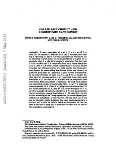
Figure 1: Possibly after a small isotopy of X in IR 3 \ {z − axis}, we can consider a regular projection π : X → C1 given by π : (r, θ, z) 7→ (1, θ, z), where C1 = {(r, θ, z)|r = 1}. The projection π(X) ⊂ C1 is isotopic to a standard projection that is constructed as follows. For n = b(X) we first consider the n circles ck = {(r, θ, z)|r = 1, z = nk } for 1 ≤ k ≤ n. Next, we alter the projection of this trivial unlink of n components to construct the projection of π(X) by having adjacent circles ci and ci+1 cross via the addition of a positive or negative crossing at the needed angle to produce a projection of X. It is clear through an ambient isotopy of IR 3 which preserves the fibers of H that we can always reposition X in IR3 \ {z − axis} so that π(X) is a standard projection. (See Figure 1 and 2.) ci+2

ci+1 ci The circles ci on a portion of the cylinder C1

−1 σi σi+1

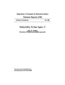
Figure 2: From a standard projection π(X) on C1 we can read off a cyclic word in the classical Artin generators σi±1 , 1 ≤ i ≤ n − 1. Specifically, β(X) is the cyclic word that comes from recording the angular occurrence of crossings where a positive (respectively negative) crossing between the circles ci and ci+1 contributes a σi (respectively σi−1 ) element to β(X), 1 ≤ i ≤ n − 1.

3

Monotonic Simplification n i+1 i 1

σi σ−1 i n

n

n

i+1

i+1

i

i

1

1

σ−1 i σi

Reidemeist type II move n

n

j+1

j+1

n

i+2

i+2

j

j

i+1

i+1

i+1

i+1

i

i

i

i

1

1

1

σi+1 σi σi+1 Reidemeister type III move

σi σi+1 σi

σi σj

1

σj σi

braid group relation for |i−j|>1

±1 ±1 σi goes to Figure 3: For type III moves there is also moves corresponding to σi−1 σi+1 ±1 ±1 −1 −1 −1 −1 −1 σi+1 σi σi+1 , and σi σi+1 σi goes to σi+1 σi σi+1 . For the braid group relations we also have the moves σiǫ σ δ goes to σjδ σiδ where ǫ, δ ∈ {−1, 1}.

We can alter π(X) (and, correspondingly, β(X)) while preserving the n-braid structure of X, plus its standard projection characteristic, by judicious use of type-II and -III Reidemeister moves and the braid group relation. (See Figure 3.) We consider the equivalence classes under the moves in Figure 3. Specifically, X and X ′ are braid isotopic if π(X) can be altered to produce π(X ′ ) through a sequence of type-II and -III moves, and braid group relations. We will let Bn (X) be notation for the equivalence class of n-braids which are braid isotopic to X. Next, let W = {σ1 , · · · , σn−2 } and U = {σ2 , · · · , σn−1 }. We now have a sequence of definitions. An n-braid X admits a destabilization if for π(X), its associated braid word β(X) is of the ±1 form W σn−1 , where W is a word using only the generators in the set W. (See Figure 4(a).) X admits an exchange move if β(X) is of the form W U where W (respectively U ) is a word using only the generators in the set W (respectively U). Alternatively, if X admits an exchange move −1 then there is a braid isotopic X ′ with β(X ′ ) of the form W1 σn−1 W2 σn−1 where W1 and W2 are words using only the generators in W. (See Figure 4(b).) Finally, X admits an elementary p ±1 W2 σn−1 where W1 and W2 are words in (braid preserving) flype if β(X) is of the form W1 σn−1 W and p ∈ Z − {0}. In Figure 4(c) we allow for the strands to be weighted. Thus, the crossings

4

William W. Menasco

Figure 4: can be seen as generalized crossings and the performance of the isotopy can products twisting in these weighted strands. We say that Bn (X) admits a destabilization, exchange move or elementary flype, respectively, if there exists a braid representative X ′ ∈ Bn (X) which admits a destabilization, exchange move or elementary flype, respectively. A long standing problem (Problem 1.84 in [K]) is determining when an n-braid equivalence class Bn (X) contains a braid X that admits either a destabilization, an exchange move, or an elementary flype. Our main result (Theorem 1) states that there is a simple algorithmic method for making these determinations. To understand this algorithm we need to consider our representation of X in H anew using ‘rectangular diagrams’.

1.2

Rectangular diagrams and main results.

A horizontal arc, h ⊂ C1 , is any arc having parametrization {(1, t, z0 )|t ∈ [θ1 , θ2 ]}, where the horizontal level, z0 , is a fixed constant and |θ1 − θ2 | < 2π. The angular support of h is the interval [θ1 , θ2 ]. Horizontal arcs inherit a natural orientation from the forward direction of the θ coordinate. A vertical arc, v ⊂ Hθ0 , is any arc having parameterization {(r(t), θ0 , z(t))|0 ≤ t ≤ 1, r(0) = r(1) = 1; and r(t) > 1, dz dt > 0 for t ∈ (0, 1)}, where r(t) and z(t) are real-valued functions that are continuous on [0, 1] and differentiable on (0, 1). The angular position of v is θ0 . The vertical support of v is the interval [z(0), z(1)]. (We remark that the parametrization

5

Monotonic Simplification of the the vertical arcs will not be used in assigning orientation to the vertical arcs.) axis

axis

(a) arc presentation

standard projection

transition between standard projection and arc presentation (b)

Figure 5: Let X be an oriented link type in S 3 . X η ∈ X is an arc presentation if X η = h1 ∪ v1 ∪ · · · ∪ hk ∪ vk where: 1. each hi , 1 ≤ i ≤ k, is an oriented horizontal arc having orientation agreeing with the components of X η , 2. each vi , 1 ≤ i ≤ k, is a vertical arc, 3. hi ∩ vj ⊂ ∂hi ∩ ∂vj for 1 ≤ i ≤ k and j (modk) = {i, i − 1}, 4. the horizontal level of each horizontal arc is distinct, 5. the vertical position of each vertical arc is distinct. 6. the orientation of the horizontal arcs will agree with the forward direction of the θ coordinate, and the orientation of the vertical arcs is assigned so as to make the components of X η oriented. For a given arc presentation X η = h1 ∪ v1 ∪ · · · ∪ hk ∪ vk there is a cyclic order to the horizontal levels of the h′i s, as determined by their occurrence on the axis, and a cyclic order to the angular position of the vj′ s, as determined by their occurrence in H. It is clear that given two arc presentations with identical cyclic order for horizontal levels and angular positions

6

William W. Menasco

there is an ambient isotopy between the two presentations that corresponds to re-scaling of the horizontal levels and angular positions along with the horizontal and angular support of the arcs in the presentations. Thus, we will think of two arc presentations as being equivalent if the cyclic orders (up to a change of indexing) of their horizontal levels and vertical positions are equivalent. We define the complexity of the arc presentation X η as being C(X η ) = k, i.e. the number of horizontal (or vertical) arcs. Given a closed n-braid X and a corresponding standard projection π(X) we can easily produce a (not necessarily unique) arc presentation X η as illustrated in transition of Figure 5. Clearly, there is also the transition from an arc presentation X η to an n-braid X with a N X η or X η −→ B X it indicate these two standard projection π(X). We will use the notation X−→ presentation transitions.

Figure 6: Illustration (a) corresponds to horizontal exchange moves and (b) corresponds to vertical exchange moves. In each of the illustrated sequences dotted arcs are used to indicate that the adjoining vertical arcs (for (a)) and horizontal arcs (for (b)) have two possible ways of attaching themselves to the labeled solid arc. We next define elementary moves on an arc presentation X η . To setup these moves we let X η = h1 ∪ v1 ∪ · · · ∪ hk ∪ vk with: zi the horizontal position for hi ; [θi1 , θi2 ] the angular support for hi ; θi the angular position for vi ; and [zi1 , zi2 ] the vertical support for vi (where 1 ≤ i ≤ k in all statements). Horizontal exchange move—Let hj and hj ′ be two horizontal arcs that are, first, consecutive and, second, nested. Namely, first, when the points (0, 0, zi ), 1 ≤ i ≤ k, are viewed on the z-axis (0, 0, zj ) and (0, 0, zj ′ ) are consecutive in the cyclic order of the horizontal levels. And second, either [θj1 , θj2 ] ⊂ [θj1′ , θj2′ ], or [θj1′ , θj2′ ] ⊂ [θj1 , θj2 ], or [θj1′ , θj2′ ] ∩ [θj1 , θj2 ] = ∅, i.e. nested.

Monotonic Simplification

7

′ Then we can replace X η with X ′η = h1 ∪ · · · ∪ vj−1 ∪ h′j ∪ vj′ ∪ · · · ∪ vj′ ′ −1 ∪ h′j ′ ∪ vj′ ′ ∪ · · · ∪ hk ∪ vk where for the corresponding horizontal positions we have zj′ = zj ′ and zj′ ′ = zj , and the vertical ′ support for vj−1 , vj′ , vj′ ′ −1 and vj′ ′ are adjusted in a corresponding manner. (See Figure 6(a).)

Vertical exchange move—Let vj and vj ′ be two vertical arcs that are again consecutive and nested. Namely, the angular positions θj and θj ′ are consecutive in the cyclic order of the vertical arcs of X η . And, either [zj1 , zj2 ] ⊂ [zj1′ , zj2′ ], or [zj1′ , zj2′ ] ⊂ [zj1 , zj2 ], or [zj1′ , zj2′ ] ∩ [zj1 , zj2 ] = ∅, i.e. nested. Then we can replace X η with X ′η = h1 ∪ · · · ∪ h′j−1 ∪ vj′ ∪ h′j ∪ · · · ∪ h′j ′ −1 ∪ vj′ ′ ∪ h′j ′ ∪ · · · ∪ hk ∪ vk where for the corresponding angular positions we have θj′ = θj ′ and θj′ ′ = θj , and the angular support for h′j−1 , h′j , h′j ′ −1 and h′j ′ are adjusted in a corresponding manner. (See Figure 6(b).) Horizontal simplification—Let hj and hj+1 be two vertical arcs that are consecutive (as defined ′ in the horizontal exchange move). Then we can replace X η with X ′η = h1 ∪ · · · ∪ vj−1 ∪ ′ ′ ′ ′ hj ∪ vj+1 · · · ∪ hk ∪ vk where: the horizontal position of hj is zj ; the angular support of hj is ′ [θj1 , θj2 ] ∪ [θ(j+1)1 , θ(j+1)2 ]; the angular position of vj−1 (respectively vj′ ) is θj−1 (respectively ′ θj ); and the vertical support of vj−1 and vj′ are adjusted correspondingly. Vertical simplification—Let vj and vj+1 be two vertical arcs that are consecutive (as defined in the vertical exchange move). Then we can replace X η with X ′η = h1 ∪· · ·∪h′j ∪vj′ ∪h′j+2 · · ·∪hk ∪ vk where: the angular position of vj′ is θj ; the vertical support of vj′ is [zj1 , zj2 ]∪ [z(j+1)1 , z(j+1)2 ]; the horizontal position of h′j (respectively h′j+2 ) is zj1 (respectively z(j+1)1 ); and the angular support of h′j and h′j+2 are adjusted correspondingly. Given an arc presentation X η we notice that for any sequence of elementary moves applied to X η , the complexity measure C(X η ) is non-increasing. That is, any sequence of elementary moves which includes the uses of either horizontal or vertical simplification will be monotonic simplification. One would hope that for a closed n-braid X which admits, respectively, a destabilization, exchange moves, or elementary flype, there exists a sequence of elementary moves to the arc N X η ) such that for the resulted arc presentation X ′η , the presentation X η (coming from X−→ B X ′ admits, respectively, a destabilization, exchange closed n-braid X ′ coming from X ′η −→ move or elementary flype (as seen from the standard projection π(X ′ )). Unfortunately, this is too good to be true. In order to produce a X ′ that admits the assumed isotopy it may be necessary to increase the number of arcs in the arc presentation. At first glance this seems to disturb our ability to maintain the characteristic of monotonic simplification. However, it is possible to control the manner in which we introduce additional arcs in the arc presentation to maintain monotonic simplification using an altered complexity measure. In particular, we have the following move for introducing additional arcs in an arc presentation. Horizontal shear—For a given arc presentation X η = h1 ∪v1 ∪· · ·∪hk ∪vk let I be a collection of

8

William W. Menasco

Figure 7: The left illustration is X η and the right is XIη . We can recover X η from XIη through a sequence of horizontal (or vertical) simplifications. The number of additional arcs allowed when we shear is undetermined.

disjoint closed angular interval of the form [θk , θk +ǫ], 0 ≤ k ≤ l such that for θ ∈ I we have that Hθ contains no vertical arc of X η . Suppose hi be a horizontal arc whose horizontal support contains intersect I. Then a horizontal shear of X η along I is new shear arc presentation XIη that is related to X η via the alterations illustrated in Figure 7. In particular, X η can be obtained from XIη via a sequence of horizontal simplifications that occur inside the angular interval I. There is no limit on the number of arcs of XIη , but the growth in arcs can only occur inside the interval I. We allow shearing on any or all of the horizontal arcs of X η whose angular support intersects the intervals of I. Given a horizontal shear XIη of X η let k′ be the number of horizontal arcs of XIη whose angular support does not intersect I. Let k′′ be the number of point of intersection between horizontal arcs and ∂I. We define the complexity measure C(XIη ) = k′ + 12 k′′ . The reader should notice that C(XIη ) = C(X η ). (We will abuse notation using C for both complexities. Thus, the reader is required to refer to the context in determining which complexity is being referenced.) Since the complexity measure for XIη does not measure the total number of arcs of XIη we can treat XIη as the equivalence class of all presentations coming from the alteration depicted in Figure 7. For our purposes we will allow I to be: a single interval {[θ0 , θ0 + ǫ]} when we are discussing whether X admits a destabilization; two disjoint intervals {[θ1 , θ1 + ǫ1 ], [θ2 , θ2 + ǫ2 ]} when we are discussing whether X admits an exchange move; and three disjoint intervals {[θ1 , θ1 + ǫ1 ], [θ2 , θ2 + ǫ2 ], [θ3 , θ3 + ǫ3 ]} when we are discussing whether X admits an elementary flype. Once the number of intervals in I has been specified it is easily observed that due to the ability to rescale the angular support of horizontal arcs and the intervals of I given X η there are combinatorially only a finite number of possible XIη . Next, we adapt the elementary moves on arc presentations to moves on XIη so as to have them be monotonic simplifications with respect to C(XIη ). First, if the horizontal arcs hj , hj ′ of our original horizontal exchange move (respectively, vertical arcs vj , vj ′ of the vertical exchange


9

move) are contained in a single interval of either [0, 2π] \ I or I, then we allow the performance of a horizontal (respectively, vertical) exchange move. Second, in a similar fashion if hj , hj+1 (respectively, vj , vj+1 ) are contained in a single interval of either [0, 2π] \ I or I then we again allow the performance of a horizontal (respectively, vertical) simplification. In both cases, if the move occurs in an interval of I the complexity of our resulting XIη is unchanged. For horizontal or vertical exchange moves, independent of what interval the move occurs in, the complexity measure is unchanged. For the simplification moves the occur in intervals of [0, 2π] \ I the complexity of the resulting XIη decreases. Thus, we achieve monotonic simplification in our uses of our previous elementary moves by restricting their application to the intervals ([0, 2π]\I)∪I.

Figure 8: Figure (a) illustrates a shear-horizontal exchange and (b) illustrates a shear-vertical simplification. Again, in each of the illustrated sequences dotted arcs are used to indicate that the adjoining vertical arcs (for (a)) and horizontal arcs (for (b)) have two possible ways of attaching themselves to the labeled solid arc. We now add two new elementary moves that utilizes the intervals of I. Shear horizontal exchange move—We refer to Figure 8(a). Let hj and hj ′ be two horizontal arcs of XIη that are consecutive and nested with respect to I. That is, first, for an interval I ⊂ [0, 2π] \ I when we consider all of the horizontal arcs of XIη the horizontal levels of hj and hj ′ are consecutive in the ordering along A. Second, the angular support of hj restricted to an interval I ⊂ [0, 2π] \ I is contained inside the angular support of hj ′ restricted to I. Then we can interchange the horizontal level of these to arcs. This is achieved by first applying a horizontal shear to the portion of hj and hj ′ that is contained in I. Thus, when we consider the resulting arc presentations an original horizontal exchange move is realizable. We abuse notation referring to the resulted arc presentation as XIη . Notice that C(XIη ) remains constant. Shear vertical simplification—We refer to Figure 8(b). Let vj be a vertical arc of XIη that are consecutive with respect to I. That is, for an interval I ⊂ [0, 2π] \ I there is no vertical arc whose angular position is between vj and I. We can then push vj into I. Again, we abuse notation by referring to the resulted arc presentation as XIη . Notice that C(XIη ) is decreased by a count of one. We are now in a position to state our main results.

10

William W. Menasco

Theorem 1 Let X be a closed n-braid such that Bn (X) admits, respectively, a destabilization, exchange move or elementary flype. Consider any arc presentation coming from the a preN X η . Then there exists a set of intervals I and a sequence of arc sentation transition X−→ presentations XIη = X 0 →X 1 → · · · →X l = XI′η such that: 1. If Bn (X) admits, respectively, a destabilization, exchange move or elementary flype then I has, respectively, one, two or three intervals. 2. X i+1 is obtained from X i via one of the elementary moves—horizontal exchange move, vertical exchange move, horizontal simplification, vertical simplification, shear horizontal exchange move, and shear vertical simplification. All of these moves are with respect to the intervals of I. 3. C(X i+1 ) ≤ C(X i ) for 0 ≤ i ≤ l. In particular, if X i →X i+1 corresponds to a horizontal, vertical or shear horizontal exchange move then C(X i ) = C(X i+1 ). If it corresponds to a horizontal, vertical or shear vertical simplification then C(X i+1 ) < C(X i ). Thus, our sequence is monotonic simplification. B X ′ admits, respec4. The closed n-braid obtained from the presentation transition XI′η −→ tively, a destabilization, exchange move or elementary flype (as seen from the standard projection π(X ′ )).

It should be readily evident that given an arc presentation X η one can generate only finitely many equivalent arc presentations through any sequence of horizontal and vertical exchange moves. As previously remarked combinatorially there are only finitely many possible choices for I (for one, two or three intervals). Thus, as equivalence classes there are only finitely many XIη . Finally, since the number of arcs of XIη in [0, 2π] \ I is fixed and bounded by the number of arcs of X η , and since our elementary moves on the arcs in [0, 2π] \ I is monotonic simplification then there are only a finite number of possible XI′η that can be produced by any sequence of elementary moves. The production of such a finite set is easily seen as algorithmic. Moreover, given an arc presentation from the cyclic order information of the horizontal levels and the vertical positions it can readily be determined whether either a horizontal or vertical simplification can be applied. Therefore, Theorem 1 implies that following corollary. Corollary 2 There exists an algorithm for deciding whether an closed n-braid is braid isotopic to one that admits either a destabilization, exchange move, or elementary flype.


11

The construction of our algorithmic solutions and the establishment of its monotonic simplification feature comes from utilizing the braid foliation machinery that was first developed in [BF, BM1, BM2, BM3] and further refined in the beautiful work of I.A. Dynnikov [D].

2

The cylinder machinery.

2.1

Destabilizing, exchange and flyping discs.

Our first objective is the give a geometric characterization for recognizing when a closed n-braid is braid isotopic to one that admits either a destabilization, exchange move or elementary flype. All geometric characterizations will depend on the existence of a specified embedded disc. Our characterizations will, in fact, occur in pairs: one for the braid presentation and one for the arc presentation.

Figure 9: Figure (a) illustrates the braid below the disc and (b) illustrates the braid above the disc. Destabilizing disc—(Braid presentation) Let X be a closed n-braid which admits a destabi±1 lization, i.e. the corresponding braid word β(X) = W σn−1 . Then there exists a destabilizing disc ∆d having the following properties. a. ∂∆d = αh1 ∪ αv1 where we have horizontal boundary αh1 ⊂ X and the vertical boundary αv1 ⊂ Hθ1 for some Hθ1 ∈ H b. ∆d ∩ X = αh1 . c. ∆d transversely intersects A at a single point v. d. αh1 intersects each disc fiber Hθ ∈ H exactly once when θ 6= θ1 . e. aθ = ∆d ∩ Hθ is a single arc having an endpoint on αh1 and v as the other endpoint. If θ = θ1 then αv1 ⊂ aθ1 . In particular, the braid fibration induces a radial foliation on ∆d . If X ′ is braid isotopic to X then we can extend the braid isotopy which takes X to X ′ to an ambient isotopy of S 3 \ A. This ambient isotopy takes ∆d to a destabilizing disc for X ′ ,

12

William W. Menasco

i.e. properties a. through e. are still satisfied. Thus, every n-braid representative of Bn (X) will have a destabilizing disc. Referring to Figure 9, in a neighborhood of the arc αv1 ⊂ ∂∆d the braid enters or exits the ∂∆d either above (Figure 9(a)) or or below (Figure 9(b)) ∆d . The destabilizing disc ∆d will correspond to a positive (respectively, negative) destabilization if near αv1 the braid is either entering above or exiting below (respectively, either entering below or exiting above) ∆v1 . ±1 (Arc presentation) Again with β(X) = W σn−1 , we consider the arc presentation coming from N η η the transition X−→ X . As usual, let X = h1 ∪ v1 ∪ · · · hk ∪ vk . Then we also have a disc, which is call an obvious destabilizing disc, that has the following properties.

a. Up to a re-ordering of the arc in the presentation, ∂∆d = h1 ∪ v1 ∪ h′2 ∪ v2′ where h′2 ⊂ h2 and v2′ ⊂ Hθ0 for Hθ0 ∈ H. b. ∆d ∩ X = h1 ∪ v2 ∪ h′2 . c. ∆d transversely intersects A at a single point v, the vertex of the foliation on ∆d . d. aθ = ∆d ∩ Hθ is a single arc having an endpoint v. Moreover, when Hθ does not contain v2 or v2′ , aθ has an endpoint on either h1 or h′2 . When Hθ does contain v1 (respectively v2′ ), v1 ⊂ aθ (respectively v2′ ⊂ aθ ). In particular, the braid fibration induces a radial foliation on ∆d . The scheme for determining whether ∆d corresponds to a positive or negative destabilization is the same for X η as it was for X. Exchange move disc—(Braid presentation) Let X be a closed n-braid which admits an exchange move, i.e. the corresponding braid word β(X) = W U . Then there exists a exchange disc ∆e having the following properties. a. ∂∆e = αh1 ∪ αv1 ∪ αh2 ∪ αv2 where we have the horizontal boundary αh1 , αh2 ⊂ X; and the vertical boundary αvi ⊂ Hθi where Hθi ∈ H, i = 1, 2. b. ∆e ∩ X = αh1 ∪ αh2 . c. In neighborhoods of αv1 ⊂ ∆e (respectively, αv2 ⊂ ∆e ) we have that the braid enters and exits above ∆e (respectively, the braid exits and enters below below ∆e ). d. ∆e transversely intersects A at a single vertex point v. e. {αh1 ∪ αh2 } ∩ Hθ 6= ∅ for Hθ ∈ H and θ 6∈ {θ1 , θ2 }. f. aθ = ∆e ∩ Hθ is a single arc having: an endpoint on v; an endpoint on αh1 ∪ αh2 when θ 6∈ {θ1 , θ2 }; and contains αvi when θ = θi , i = 1, 2. In particular, the braid fibration induces a radial foliation on ∆e .


13

If X ′ is braid isotopic to X then we can extend the braid isotopy which takes X to X ′ to an ambient isotopy of S 3 \ A. This ambient isotopy takes ∆e to a exchange disc for X ′ , i.e. properties a. through e. are still satisfied. Thus, every n-braid representative of Bn (X) will have an exchange disc. (Arc presentation) Again with β(X) = W U , we consider the arc presentation coming from the N X η . As usual, let X η = h ∪ v ∪ · · · h ∪ v . Then we also have a disc, which transition X−→ 1 1 k k is call an obvious exchange disc, that has the following properties. a. Up to a re-ordering of the arc in the presentation, ∂∆e = h′1 ∪ v1′ ∪ h′2 ∪ v2′ where h′1 and h′2 are subarcs of two different horizontal arcs of X η and vi′ ⊂ Hθi for Hθi ∈ H, i = 1, 2. b. ∆e ∩ X = h′1 ∪ h′2 . c. In neighborhoods of v1′ , v2′ ⊂ ∆e we have that the braid either enters (for v1′ ) and exits (for v2′ ) above ∆e , or enters (for v1′ ) and exits (for v2′ ) below ∆e . d. ∆e transversely intersects A at a single vertex point v. e. aθ = ∆e ∩ Hθ is a single arc having an endpoint v. Moreover, when Hθ does not contain vi′ , aθ has an endpoint on either h1 or h′2 . When Hθ does contain v1′ (respectively v2′ ), v1′ ⊂ aθ (respectively v2′ ⊂ aθ ). In particular, the braid fibration induces a radial foliation on ∆d . Elementary flyping disc—(Braid presentation) Let X be a closed n-braid which admits an p ±1 elementary flype, i.e. the corresponding braid word β(X) = W1 σn−1 W2 σn−1 . Then there exists a flyping disc ∆f having the following properties. a. ∂∆f = αh1 ∪αv1 ∪αh2 ∪αv2 ∪αh3 ∪αv3 where we have the horizontal boundary αh1 , αh2 , αh3 ⊂ X; and the vertical boundary αvi ⊂ Hθi where Hθi ∈ H, i = 1, 2, 3. b. ∆f ∩ X = αh1 ∪ αh2 ∪ αh3 . c. In neighborhoods of αv1 , αv2 ⊂ ∆e we have that the braid either αv1 enters and αv2 exits above ∆f , or enters αv1 and exits αv2 below ∆f . d. X admits a positive flype (respectively, negative) if in a neighborhood of αv3 the braid either enters above or exits below ∆f (respectively, enters below or exits above ∆f ). e. ∆f transversely intersects A at a single vertex point v. f. {αh1 ∪ αh2 ∪ αh3 } ∩ Hθ 6= ∅ for Hθ ∈ H and θ 6∈ {θ1 , θ2 , θ3 }.

14

William W. Menasco g. aθ = ∆f ∩ Hθ is a single arc having: an endpoint on v; an endpoint on αh1 ∪ αh2 ∪ αh3 when θ 6∈ {θ1 , θ2 , θ3 }; and contains αvi when θ = θi , i = 1, 2, 3. In particular, the braid fibration induces a radial foliation on ∆f .

If X ′ is braid isotopic to X then we can extend the braid isotopy which takes X to X ′ to an ambient isotopy of S 3 \ A. This ambient isotopy takes ∆f to a flyping disc for X ′ , i.e. properties a. through e. are still satisfied. Thus, every n-braid representative of Bn (X) will have an flyping disc. ±1 (Arc presentation) Again with β(X) = W1 U W2 σn−1 , we consider the arc presentation coming N η η from the transition X−→ X . As usual, let X = h1 ∪ v1 ∪ · · · ∪ hk ∪ vk . Then we also have a disc, which is call an obvious flyping disc, that has the following properties.

a. Up to a re-ordering of the arc in the presentation, ∂∆f = h′1 ∪ v1′ ∪ h′2 ∪ v2′ ∪ h′3 ∪ v3′ where h′1 , h′2 , h′3 are subarcs of differing horizontal arcs of X η , and vi′ ⊂ Hθi for Hθi ∈ H, i = 1, 2, 3. b. ∆f ∩ X = h′1 ∪ h′2 ∪ h′3 . c. In neighborhoods of v1′ , v2′ ⊂ ∆e we have that the braid either v1′ enters and v2′ exits above ∆f , or v1′ enters and v2′ exits below ∆f . d. X admits a positive flype (respectively, negative) if in a neighborhood of v3′ the braid either enters above or exits below ∆f (respectively, enters below or exits above ∆f ). e. ∆f transversely intersects A at a single vertex point v. f. aθ = ∆f ∩ Hθ is a single arc having an endpoint v. Moreover, when Hθ does not contain vi′ we have aθ has an endpoint on either h′1 , h′2 , or h′3 . When Hθ does contain vi′ , vi′ ⊂ aθ , i = 1, 2, 3. In particular, the braid fibration induces a radial foliation on ∆f . We will establish Theorem 1 by establishing the following proposition Proposition 3 Let X be a closed n-braid such that Bn (X) admits, respectively, a destabilization, exchange move or elementary flype. Consider any arc presentation coming from the a N X η . Then there exists a set of intervals I and a sequence of arc presentation transition X−→ presentations XIη = X 0 →X 1 → · · · →X l = XI′η such that: 1. If Bn (X) admits, respectively, a destabilization, exchange move or elementary flype then I has, respectively, one, two or three intervals.


15

2. X i+1 is obtained from X i via one of the elementary moves—horizontal exchange move, vertical exchange move, horizontal simplification, vertical simplification, shear horizontal exchange move, and shear vertical simplification. All of these moves are respect to the intervals of I. 3. C(X i+1 ) ≤ C(X i ) for 0 ≤ i ≤ l. In particular, if X i →X i+1 corresponds to a horizontal, vertical or shear vertical exchange move then C(X i ) = C(X i+1 ). If it corresponds to a horizontal, vertical or shear vertical simplification then C(X i+1 ) < C(X i ). Thus, our sequence is monotonic simplification. 4. If Bn (X) admits, respectively, a destabilization, exchange move or elementary flype then here exists an obvious, respectively, destabilizing, exchange, or flyping disc ∆ε , ε ∈ {d, e, f } for XI′η such that the angular position of the vertical boundary arcs of ∆ε occur are in the set of angles ∂I. The proof of Proposition 3 requires the development machinery for “notch discs”.

2.2

Notch discs.

We now develop our machinery further. Let X be a closed n-braid presentation that is braid isotopic to a braid that admits either a destabilization, exchange move or elementary flype. Let ∆ε then be an appropriate disc illustrating the move, i.e. for X we have ∆ε with ε ∈ {d, e, f }. N X η , and consider the impact Next, we take a transition from a braid to a arc presentation, X−→ of this transition on ∆ε . (Again, we refer to the union of arcs X η = h1 ∪ v1 ∪ · · · ∪ hk ∪ vk . The reader should refer to the descriptions of ∆ε so as to recall the understanding of the horizontal and vertical portions of ∂∆ε .) As before, we denote the leaves of the radial foliation of ∆ε by aθ (= ∆ε ∩ Hθ ); and aθ contains a vertical boundary arc when θ is θi where i = {1, 2, 3}. Since X can be positioned to be arbitrarily close to X η (where closeness is measured by the standard metric for the (r, θ, z) coordinates), by an ambient isotopy of S 3 that preserves the boundary and foliation properties of ∆ε , we can assume that X η intersects ∆ε such that the following: i. For each leaf aθ where θ 6∈ {θ1 , θ2 , θ3 } we have that aθ intersects either the interior of a single horizontal arc or the interior of a single vertical arc of X η . ii. For aθ with θ 6∈ {θ1 , θ2 , θ3 }, if aθ intersects the interior of a horizontal arc of hi ⊂ X η then aθ ∩ hi is a transverse intersection at a single point. iii. For aθ with θ 6∈ {θ1 , θ2 , θ3 }, if aθ intersects the interior of a vertical arc of vj ⊂ X η then vj ⊂ aθ .

16

William W. Menasco

iv. For the leaves aθi , i ∈ {1, 2, 3}, recall we have αvi ⊂ aθi . There are two horizontal arcs hi1 , hi2 ⊂ X η such that a. aθi ∩ X η = aθi ∩ {hi1 ∪ hi2 } b. αvi has its endpoints on hi1 and hi2 .

Figure 10: In illustrate (a) we have drawn ∆ηε ⊂ ∆ε . In (b) we indicate what the structure of ∂∆ηε . With these conditions holding we can notch ∆ε to produce ∆ηε . That is, ∆ηε ⊂ ∆ε is the sub-disc whose boundary is obtain by projecting X ∩ ∆ε along the leaves aθ to X η ∩ ∆ε . (See Figure 10.) The boundary of ∆ηε is then a union of three types of arcs: horizontal arcs, hηj , that can be either arcs or sub-arcs of the horizontal arcs of X η ; vertical arcs, vjη , that are in fact arcs coming from the vertical arcs of X η ; and vertical boundary arcs, αηθi , that can be seen as sub-arcs of the leaves aθi ⊂ ∆ε for i ∈ {1, 2, 3}. (We will let 1 ≤ j ≤ l.) We then have ∂∆ηε the sequenced union of arcs alternating between horizontal and vertical, i.e. ∂∆ηε = hη1 ∪ v1η ∪ · · · ∪ hηj1 ∪ αηθ1 ∪ hηj1 +1 ∪ · · · ∪ hηjp ∪ αηθp ∪ hηjp +1 ∪ · · · ∪ hηl ∪ vlη , p ∈ {1, 2, 3}. Extending our notation for the transition between braid presentations and arc presentations, N (X η , ∆η ) and (X η , ∆η )−→ B (X, ∆ ) for indicating the transition between we will use (X, ∆ε )−→ ε ε ε presentation-disc pairs. Clearly, given a pair (X η , ∆ηε ) when elementary moves are applied to X η there can be an alternation to either the positioning of ∆ηε or the arc decomposition of ∂∆ηε .


17

Lemma 4 (First simplication of (X η , ∆ηε )) Let X be a closed n-braid such that Bn (X) admits, respectively, a destabilization, exchange move or elementary flype and let ∆ε be, respectively, a destabilizing disc, exchange move disc, or elementary flyping disc, i.e. ε ∈ {d, e, f }. N (X η , ∆′η ) we have Then there exists an alternate disc ∆′ε such that for (X, ∆′ε )−→ ε a. X η is unchanged. η η η η η η b. ∂∆′η ε = h1 ∪ αθ1 ∪ h2 ∪ v2 ∪ · · · ∪ hl ∪ vl when ε = d. η η η η η η c. ∂∆′η ε = h1 ∪ αθ1 ∪ h2 ∪ v2 ∪ · · · ∪ hl ∪ αθ2 when ε = e. η η η η η η η η η η d. ∂∆′η ε = h1 ∪ αθ1 ∪ h2 ∪ αθ2 ∪ h3 ∪ v3 ∪ · · · ∪ h4 ∪ v4 ∪ · · · ∪ hl ∪ αθ3 when ε = f .

Proof. The statements [b.] through [d.] are achieved by performing a isotopy of the arcs ′ αηθi s. In particular, statement [b.] is true by construction. To achieve statement [c.] while maintaining the truth of statement [a.] we start with the vertical boundary arcs of ∆ηε , αηθ1 , αηθ2 . If these two arcs have endpoints on a common horizontal arc of X η then we are done. If not then we push αηθ2 backward (or forward) through the disc fibers of H. This push will naturally isotop αηθ2 in the disc fibers. We stop our push when αηθ2 has an endpoint on a horizontal arc that αηθ1 also has an endpoint on. This corresponds to an ambient isotopy of the graph X η ∪ αηθ1 ∪ αηθ2 in IR3 \ A. There is still a disc whose boundary is the union of two subarc and ′η the resulting two vertical boundary arcs. This new disc is our ∆′η ε . It is easy to see that ∆ε is in fact a notch disc. Similarly, for achieving statement [d.] while maintaining the truth of statement [a.] we first push αηθ2 backward until it has an endpoint on a horizontal arc that also contains an endpoint of αηθ1 . Not we push αηθ3 backward until it has an endpoint on a horizontal arc that contains an endpoint of αηθ2 . Since both pushes are ambient isotopies of IR 3 \ A we again have an new notch disc. ♦ ′η We will refer to the portion hη2 ∪ v2η ∪ · · · ∪ hηl ∪ vlη ⊂ ∂∆′η d as the middle boundary of ∆d . ′η η η η η η (The middle boundary of ∂∆′η e and ∂∆f is, respectively, h2 ∪ v2 ∪ · · · ∪ hl and h3 ∪ v3 ∪ · · · ∪ hη4 ∪ v4η ∪ · · · ∪ hηl .) Proposition 3 and, thus, Theorem 1 will be established when the middle boundary of ∆ηε has been simplified so that it contains only a single horizontal boundary arc.

For the remainder of our discussion we will assume that our notch disc satisfies the conclusion of Lemma 4.

2.3

The intersection of C1 & ∆ηε .

In this subsection we start with a given initial pair (X η , ∆ηε ) and analyze the intersection C1 ∩ ∆ηε . Our overall strategy is to simplify C1 ∩ ∆ηε until ∆ηε is an obvious disc illustrating

18

William W. Menasco

either a destabilization, exchange move or elementary flype. We consider the intersection C1 ∩ ∆ηε . Notice that for each horizontal arc hηj ⊂ ∂∆ηε we necessarily have hηj ⊂ C1 ; for each vertical arc vjη ⊂ ∂∆ηε we have vjη ∩ C1 = ∂vjη ; and we can assume that the vertical boundary arcs αηθi transversally intersects at finitely many points. We can assume that C1 and int(∆ηε ) intersect transversely. Thus, C1 ∩ ∆ηε is a union of simple arcs (sa ) and simple closed curves (scc ). This next lemma allows us to get some initial control over the behavior of C1 ∩ ∆ηε without altering X η . The reader should refer back to the notation in Lemma 4 and our notion of the middle boundary of ∂∆ηε . Lemma 5 (Second simplication of (X η , ∆ηε )) Let (X, ∆ε ) be a braid presentation/disc pair where ε ∈ {d, e, f }, and consider an arc presentation/disc pair coming from the transition N (X η , ∆η ). Then we can replace the pair (X η , ∆η ) with (X η , ∆′η ) such that no sa (X, ∆ε )−→ ε ε ε ′η ∩ C have their endpoints on the . In particular, all sa of ∆ has an endpoint on X η ∩ ∂∆′η ε ε 1 ′η vertical boundary curves of ∂∆ε . Proof. By an isotopy of a collar neighborhood of ∂∆ηε in ∆ηε we can assume that there is a ′η η neighborhood N ⊂ ∆ηε which has the structure (X η ∩ ∂∆′η ε ) × I such that N ∩ C1 = X ∩ ∂∆ε . After this isotopy the only place where any sa can have its endpoints is on the vertical boundary arcs. ♦ Next, we set T0 = {(r, θ, z)|r < 1} and T∞ = {(r, θ, z)|r > 1}. Let δ ⊂ ∆ηε \ (C1 ∩ ∆ηε ) be any component. If δ ⊂ T0 (respectively δ ⊂ T∞ ) then we assign δ a “0” (respectively “∞”) label, i.e. δ0 (respectively δ∞ ). Lemma 6 (Initial position of C1 ∩ ∆ηε -part 1.) Let (X, ∆ε ) be a braid presentation/disc pair where ε ∈ {d, e, f }, and consider an arc presentation/disc pair coming from the transiN (X η , ∆η ). Then we can replace the pair (X η , ∆η ) with (X η , ∆′η ) such that the tion (X, ∆ε )−→ ε ε ε following hold: ′η a. Every scc of C1 ∩ ∆′η ε bounds a subdisc of ∆ε whose associated label is 0.

b. For every scc of c ⊂ C1 ∩ ∆′η ε either c bounds a subdisc of C1 which contains a single η horizontal arc of X , or c bounds the unique subdisc of ∆ηε which is intersected by A. η c. Every sa of C1 ∩ ∆′η ε having both endpoints on the same vertical boundary arc αθi , 1 ≤ ′η i ≤ 3, is outer-most in ∆′η ε and splits off a subdisc of ∆ε whose associated label is 0. η d. For every sa γ ⊂ C1 ∩ ∆′η ε that has both endpoints on the same αθi , 1 ≤ i ≤ 3, there exists a sub-arc γ ′ ⊂ Hθi ∩ C1 such that γ ∪ γ ′ bounds a subdisc of C1 that intersects exactly one horizontal arc of X η .


19

′η Proof. To establish statement a. we consider an scc c ⊂ C1 ∩ ∆′η ε and let R ⊂ C1 ∩ ∆ε be the disc region with c = ∂R. We let ∆c ⊂ C1 be the sub-disc having c = ∂∆c . Suppose that R contains a sub-region having an associated label ∞; and assume with respect to ∆c c is the innermost such scc , i.e. if there is any scc c′ ⊂ C1 ∩ R then c′ bounds a sub-disc of R having a single associated label 0. We now take a push-off of the open disc int(∆c ) ⊂ C1 into T0 to produce a disc ∆′c which has ∆′c ∩ C1 = ∂∆′c = c. By our innermost assumption on c we can assume that ∆′c ∩ R = c. Thus, the 2-sphere ∆′c ∩c R is embedded in the complement of our arc presentation X η and, thus, bounds a 3-ball. We can then use this 3-ball to isotop R to ∆′c . This isotopy will be eliminate all of the scc intersection of int(R) ∩ C1 . Continuing in this fashion we can assume that statement a. holds.

To establish statement b. let c ⊂ C1 ∩ ∆ηε . Assume that c bounds a sub-disc R ⊂ ∆ηε . Now that we have established the validity of statement a. we can assume that int(R) ⊂ T0 . Let ∆c ⊂ C1 having ∂∆c = c. We now isotop R by radially pushing R out of T0 along θ-rays. The obstruction to pushing R totally out of T0 will be horizontal arcs of X η that are contained in ∆c . Thus, this radially isotopy of R will result in a new scc for each horizontal arc of ∆c ∩ X η . The arguments establishing statements c. & d. are similar. For statement c. let a ⊂ C1 ∩∆ηε be a sa that splits off a region R ⊂ ∆ηε . Assume for convenience that ∂a are contained in the vertical boundary arc αηθ1 ⊂ Hθ1 where Hθ1 ∈ H. Let ∆a ⊂ C1 be the half-disc such that ∂∆a = a ∪ b where b is an arc contained in Hθ1 . Suppose that there is a portion of R that has the associated label ∞. Moreover, assume with respect to ∆a that c is an outermost having such a labeled region R. That is, for every other sa in C1 ∩ int(R) they split off a sub-disc that is a half-disc only intersects T0 . Under these assumption we can construct a 2-sphere bounding a 3-ball that gives us an isotopy reducing the number of intersections of C1 ∩ int(R). Specifically, we push off int(∆a ) into T0 . Call this new half-disc ∆′a . Since a is outermost with respect to ∆a we can assume that ∆′a ∩ R = a. Now, ∆′a ∪a R is an embedded disc in the complement of X η having its boundary a curve ca ⊂ Hθ1 . Let δca ⊂ Hθ1 that has ca as its boundary. Then δca ∪ca (∆′a ∪a R) is an embedded 2-sphere. Since X η can only intersect Hθ1 positively and since the algebraic intersection of X η with any 2-sphere is zero, this embedded 2-sphere must in fact be in the complement of X η . Thus, we have our needed 2-sphere bounding a 3-ball. If we restrict our attention to Hθ1 we see that the isotopy through this 3-ball will take the arc R ∩ Hθ1 to the arc ∆′a by pushing through the disc δca . Thus, we achieve statement c. Finally, to achieve statement d. we again use an isotopy that radially pushes out any halfdisc that is split off in ∆ηε by an outermost sa . The obstruction to pushing these half-discs out of T0 will be portions of horizontal arcs. The statement follows. ♦ Lemma 7 (Initial position of C1 ∩ ∆ηε -part 2.) Let (X, ∆ε ) be a braid presentation/disc

20

William W. Menasco

pair where ε ∈ {d, e, f }, and consider an arc presentation/disc pair coming from the transiN (X η , ∆η ). We can replace the pair (X η , ∆η ) with (X η , ∆′η ) such that for every tion (X, ∆ε )−→ ε ε ε ′η η = ∅ then δ is a disc of component of δ ⊂ ∆′η \ (C ∩ ∆ ) with label 0, if δ ∩ A = ∅ and δ ∩ X ε ε 1 the one of the following type: a. A whole disc–A disc whose boundary in C1 ∩ ∆′η ε is a scc . b. A half disc–A disc whose boundary is the union of two arc γ1 ∪ γ2 where γ1 ⊂ C1 ∩ ∆ηε and γ2 ⊂ αηθi for some i ∈ {1, 2, 3}. c. a rectangle–A disc whose boundary is the union of four arcs γ1 ∪ γ2 ∪ γ3 ∪ γ4 where γ1 , γ3 ⊂ C1 ∩ ∆ηε , γ2 ⊂ αηθi and γ4 ⊂ αηθj for 1 ≤ i < j ≤ 3. Moreover, there exists arcs γ2′ ⊂ Hθi ∩ C1 and γ4′ ⊂ Hθj ∩ C1 such that γ1 ∪ γ2′ ∪ γ3 ∪ γ4′ bounds a disc in C1 which intersects exactly one horizontal arc which intersects both γ2′ and γ4′ . . Proof. Statements a. (concerning the whole disc) and b. (concerning the half disc) clearly following, respectively, from statements a. plus b. and c. plus d. of Lemma 6. Finally, if there exists a horizontal arc h ⊂ X η that intersects at least two components of I then would we try and “push” ∆ηε out of T0 it will obstruct a rectangular disc as described in statement c. ♦ Lemma 8 (Initial position of C1 ∩ ∆ηε -part 3.) Let (X, ∆ε ) be a braid presentation/disc pair where ε ∈ {d, e, f }, and consider an arc presentation/disc pair coming from the transition N (X η , ∆η ). We can replace the pair (X η , ∆η ) with (X η , ∆′η ) such that no component (X, ∆ε )−→ ε ε ε of ∆′η ∩ T is a rectangle subdisc as described in conclusion [c.] of Lemma 7. ε 0 Proof. Referring to the description of a rectangle subdisc in conclusion [c.] of Lemma 7 suppose we have a disc in R ⊂ ∆ηε ∩ T0 whose boundary is the union of four arcs γ1 ∪ γ2 ∪ γ3 ∪ γ4 where γ1 , γ3 ⊂ C1 ∩ ∆ηε , γ2 ⊂ αηθi and γ4 ⊂ αηθj for 1 ≤ i < j ≤ 3. We then have a rectangle disc R′ ⊂ C1 such that ∂R′ = γ1 ∪ γ2′ ∪ γ3 ∪ γ4′ where γ2′ ⊂ Hθi ∩ C1 and γ4′ ⊂ Hθj ∩ C1 . Moreover, there is a horizontal arc of X η which intersects both γ2′ and γ4′ . We can then push R′ slightly into T∞ to produce a rectangle R′′ such that ∂R′′ = γ1 ∪ γ2′′ ∪ γ3 ∪ γ4′′ where γ2′′ ⊂ Hθi and γ4′′ ⊂ Hθj . The reader should observe that since R′ was intersected by a single horizontal arc across its entire angular length R′′ does not intersect X η . Our new ∆′η ε is obtained by cutting η ′′ ′′ out R in ∆ε and replacing it with R . We can then smooth out R to eliminate the intersection arcs γ1 & γ3 . ♦ In Lemmas 5, 6 and 7 for the pair (X η , ∆ηε ) we did not alter X η , only ∆ηε . Thus, our complexity measure C(X η ) remained constant. The resulting pair (X η , ∆′η ε ) coming from the


21

application of Lemmas 6, 7 and 8 will be referred to as an initial position for the braid presentation/disc pair.

2.4

The tiling machinery on ∆ηε .

We now make the transition from an arc presentation to a shear presentation. To do this we need to specify the intervals for I. This is achieved by specifying the angular support of the vertical boundary arcs. N (X η , ∆η ) produces a pair that So given (X, ∆ε ) we assume that the transition (X, ∆ε )−→ ε satisfies the conclusion of Lemma 4 & 5. With this assumption in place we now refer back to the pair (X, ∆ε ).

For a vertical boundary arc αθi ⊂ ∂∆ε , either braid entering or braid exiting. (See Figure 9.) If αθi is braid entering then [θi , θi + ǫ] ∈ I. If αθi is braid exiting then [θi − ǫ, θi ] ∈ I. With S (X η , ∆η ) for going this assignment for I in place introduce new transition notation (X, ∆ε )−→ ε I from a braid/disc pair to a shear-arc-presentation/notch-disc pair. We now adapt the classical foliation/tiling machinery of surfaces in braid structures extensively developed and exploited in [BM1, BM2, BM3, BM4, BF]. This machinery has built into it the ability to recognize when and where exchange moves are admitted. To start our adaptation we have the following definitions. Given a pair (XIη , ∆ηε ) in initial position (as specified by the conclusions of Lemma 6, 7 & 8), let hηi ⊂ XIη be a horizontal arc that intersects at most one of the interval components of I. Let h ⊂ hηi be a component of hηi ∩([0, 2π)\I). Let [θ1h , θ2h ] be the angular support of h and z h be the vertical position of h. The coning disc of h is the disc δh = {(r, θ, z h )|0 ≤ r ≤ 1, θ1h ≤ θ ≤ θ2h }. Let vh = δh ∩ A is the vertex for δh . The reader should notice that a coning disc inherits a radial foliation from its intersection with the disc fibers of H. Now for any coning disc δh we consider the intersection set ∆ηε ∩ δh . By the three Lemmas used to define initial position we know that this intersection set will be a union of arcs that are transverse to disc fibers of H and, thus, the leaves of the radial foliation of δh . So viewed in δh any arc of intersection with ∆ηε can be viewed as parallel to h ⊂ ∂δh . In particular, by possibly a slight isotopy of the whole discs, half discs and rectangles of ∆ηε ∩ T0 , we can assume that the cylindrical coordinates of any intersection arc in the set ∆ηε ∩ δh has constant r-coordinate along with constant z-coordinate being z h . Let γ ⊂ ∆ηε ∩ δh such the intersection arc in δh having the smallest r-coordinate which we call rγ . We can then isotop γ through δh and past the axis A by letting rγ go to zero (and past it) to produce a disc T∆ηε that has a tiled foliation. By dragging ∆ηε along we can extend this isotopy of ∆ηε . As illustrated in Figure 11 there are two cases for this tiling isotopy.

22

William W. Menasco

Figure 11: The corresponding alteration in the foliation in (a) is depicted in Figure 12(a). Similarly, there is a correspondence between illustration (b) and Figure 12(b). The curve cγ is used to designate the grouping of the vertices and singularities introduced by the tiling isotopy that is associated with the intersection arc γ.

6 ∅). In Figure 11(a) we have the case where h is in fact the horizontal arc hηi (i.e. hηi ∩ I = η Here the tiling isotopy introduces to intersection points or vertices of ∆ε with A; and two of tangency points with disc fibers of H or singular points. In Figure 11(b) we have the case where h has an endpoint in a component of I. Here the tiling isotopy will isotopy one of the vertical boundary arcs of αθi of XIη . This will introduce two points of intersection of αθi with A and one tangency point with a disc fiber of H which we again call a singular point. Figure 11 also has the corresponding alteration to the foliation of ∆ηε . For convenience we will assume in all situations that the singularities introduces in tiling isotopy does not occur in a disc fiber of H that contains a vertical arc or vertical boundary arc. We will use the notation η η T η T η T η T η T (X (XIη , ∆ηε )−→ I , ∆ε ) to indicate the tiling isotopy between (XI , ∆ε ) and (XI , ∆ε ). In order that we maintain the grouping of the vertices and singularities introduced by tiling isotopy we will designate in the foliation a curve cγ ⊂ T∆ηε which is either a circle or an arc as illustrated in Figure 11. Specifically, when cγ is a circle it will encircle the two vertices and pass through the two singularities. When cγ is an arc it will split-off the two vertices that are on the vertical boundary arc and will pass through the single singularity. In Figure 12 we see how the tiling isotopy alters the radial foliation in a neighborhood of the intersection arc γ.


23

Figure 12: The parity signs indict one possibility for the parity assignment of singularities and vertices. In illustration (a) there is always the occurrence of a positive/negative pair of vertices and singularities. In illustration (b) there is always the occurrence of a positive/negative pair of vertices. The lone singularity can be of either parity. The curves cγ maintain the grouping of the vertices and singularities introduced by the tiling isotopy associated with the intersection arc γ. To review a little more thoroughly the tiling machinery, we consider the orientations of the axis A, our disc ∆ηε and the disc fibers of H (which is consistent with the orientation of A). We can associate to each vertex and singularity a parity as follows. A vertex v ⊂ T∆ηε ∩ A is positive (or +) if v is a positive intersection. Otherwise, v is negative (or −). A singular point s ⊂ T∆ηε is positive (or +) if the orientation of the tangent plane to ∆ηε at s agrees with the orientation of the disc fiber of H that contains s. Otherwise, s is negative (or −). Keeping with the literature that has developed around this topic of tiled foliation, we will refer to the non-singular leaves that have an endpoint on TXIη and another endpoint a vertex as a-arcs, and non-singular leaves that have both endpoints being vertices as b-arcs. There are four naturally occurring simply connected graphs contained in ∆ηε . (Refer to Figure 12.) For µ, ν ∈ {+, −} the graph Gµ,ν is described as follows: 1. The vertices of Gµ,ν are all the µ vertices in the tiling foliation of ∆ηε . 2. Each edge of Gµ,ν is contained in a tile that has a ν singular point. 3. Moreover, each ν singular point is contained in an edge of Gµ,ν . 4. For G+,ν the endpoints of its edges are all + vertices. 5. For G−,ν the endpoints of its edges are either ν vertices or points on horizontal arc of XIη . Briefly, we state a few salient properties of the graphs Gµ,ν which we will reference as ⋆-properties. (The most consolidated reference for these properties is [BF].) i. By construction every vertex of the tiling foliation is in either G+,+ or G−,− (respectively, G+,− or G−,+ ).

24

William W. Menasco

Figure 13: There are three possible means by which a singularity can be formed. In column (i) two b-arcs (leaves in the foliation that have both endpoints on vertices) can come together to form a singularity. In column (ii) the neighborhood of the singularity has both a-arcs (leaves having an endpoint on a vertex and an endpoint on the boundary of ∆ηε ) and b-arcs. In column (iii) the singularity has its vertices endpoints on a vertical boundary arc. ii. The graphs G+,+ and G−,− (respectively, G+,− and G−,+ ) are disjoint. iii. All four graphs are simply connected. Thus, every component of G−,− (respectively, G−,+ ) has a unique edge that has an endpoint on a horizontal arc of TXIη . iv. The number of negative vertices is one less than the number of positive vertices. v. Each − vertex that is in the interior of T∆ηε (i.e. not on a vertical boundary arc) is the endpoint of an edge in G−,− and an edge in G−,+ . (Remark: With an appropriate understanding of “interior” a similar statement can be may for + vertices.) The combinatorics tiling foliation machinery as developed in [BM1, BM2, BM3, BM4, BF] inherently has the ability to recognize when and where we should be applying our elementary moves. Specifically, we have the following tiling operations. O1 –Using the foliation to detect horizontal exchange moves. There are three differing configurations of the tiling foliation can be used to detect the occurrence of a horizontal exchange move. We now go through each configuration. In each case the application a horizontal exchange


25

move will either maintain or reduce the number of cγ curves.

Figure 14: In (a) we depict the tiling foliation in a neighborhood of a valence two vertex and show the alternation to the foliation when we eliminate positive/negative pairs of vertices and singularities. In (b) see illustrate a cross-section of the neighborhood in (b) along with the cross-section of the coning disc δh and the cylinder C1 . O1.1 –Configuration: an interior valence two vertex. Let v0 be the endpoint vertex of Gµ,− and Gµ,+ . (For clarity of discussion we focus on the case where µ is negative.) Thus, v1 is adjacent to exactly two singular leaves. Figure 14(a) illustrates the foliated disc neighborhood that contains the two positive vertices, v2 and v3 , and the two singularities (which have differing parities), s+ and s− . By construction of the tiling foliation there is a cγ curve that passes through the two singularities and encircles v1 along with one of the positive vertices, say v2 . Thus, between v1 and v2 on the axis A there is a vertex, vh , of coning disc δh for a horizontal arc h ⊂ XIη . By construction we know that the angular support of h is arbitrarily close to the angular interval between s+ and s− that overlaps the angular support of h. We can perform that classical exchange move of [BM1, BM2, BM3, BM4, BF] that would isotopy δh so that z h is near v3 and on the interval of A that is bounded by v2 and v3 . Our difficulty is in seeing that this in fact corresponds to horizontal exchange move as defined in §1.2. In particular, we consider the cone discs that have their coning point at a height on the axis A between v1 and v3 and the angular support of their associate horizontal arcs overlapping the angular support of h. Over the angular support of h the disc region in the tiled foliation of T∆ηε that is foliated by the leaves that have v1 and v3 separates vertical arcs of XIη into two classes. (The reader

26

William W. Menasco

can refer to the cross-sectional illustration in Figure 14(b).) Every vertical arc in this angular interval will either have vertical support that is in the interval [v1 , v3 ] or the interval [v3 , v2 , v1 ] (i.e. the interval containing v2 with endpoints v3 and v1 ). Thus, over the angular support of h the vertical arcs having vertical support inside [v1 , v3 ] satisfy the nested condition need for performing a vertical exchange move with any vertical arc that has its vertical support in the interval [v3 , v2 , v1 ]. We can then perform a sequence of vertical exchange moves on any and all vertical arcs that have vertical support in interval [v1 , v3 ] and angular position inside the angular support of h, so as to eliminate any such vertical arcs. (This isotopy will not alter the tiling foliation of T∆ηε , but may alter the cyclic order of the singularities in H.) This will make the angular support of h to be contain in the angular support of all horizontal arcs of TXIη whose horizontal position contain in [v1 , v3 ]. Thus, we will have the need nested condition so that when we perform the classical exchange move depicted in Figure 14 it will correspond to the horizontal exchange move of §1.2. Once the exchange move has been performed the interval [v2 , v1 ] ⊂ A will no long contain any vertex of a coning disc and we can perform the classical cancellation of positive/negative vertices and singularity pair. (See [BF].) The tiling foliation alteration is illustrated in Figure 14(a). The reader should observe that the classical exchange move is not concerned with number of coning disc vertices contained in the interval [v1 , v2 ] ⊂ A. Although initially there is only one coning disc vertex in the axis interval, after performing some number of horizontal exchange move predicated on the occurrence of a valence two vertex it is possible that the elimination of a valence two vertex may require the exchange move isotopy of numerous coning discs. The above discussion on establishing the nested condition for both vertical and horizontal exchange moves carries through in this more general setting. O1.2 –Configuration: a valence two vertex near boundary. We refer to Figure 15(a). The salient

Figure 15: The left sequence illustrates the use of a horizontal exchange move in the elimination of a valence two vertex and a cγ curve that is “near” the boundary of T∆ηε . The right sequence illustrates a horizontal exchange move that alters T∆ηε near TXIη . features of this configuration are: i) a positive vertex v that is the endpoint of G+,+ and G+,− ; ii)


27

v+ is the endpoint of leaves that are a-arcs; and in fact, iii) all of the a-arcs adjacent to v+ have an endpoint on a single horizontal arc h0 ⊂ XIη . All b-arcs adjacent to v+ will have an endpoint on a single negative vertex v− . Figure 15 depicts the cγ curve that encircles the vertices v+ and v− and passes through positive and negative singularities that are adjacent to v+ . We label the two angle at which these singularities occur as θ1 and θ2 . We make the simplifying assumption that there is no vertical arc having an angular position between θ1 and θ2 and vertical support nested in the vertical position of h0 and v+ . (This simplifying assumption can be achieved using vertical exchange moves based upon the configuration illustrated in Figure 16(b). See below.) For any horizontal arc that has angular support between θ1 and θ2 and vertical position between the position of v+ and v− we can then perform a horizontal exchange move that results in their vertical position being below that of h0 as illustrated in the sequence in Figure 15(a). Once such horizontal exchange moves are accomplished there will no longer be any vertices of coning discs on A in the interval between v+ and v− . We can thus eliminate these vertices and the two singularities that cγ passes through. This then eliminates the occurrence of this cγ . O1.3 –Configuration: horizontal arc parallel to a cγ curve. We refer to Figure 15(b) for this configuration. Let R ⊂ T∆ηε be a rectangular region that satisfies the following: i) int(R) ∩ C1 = ∅; ii) ∂R = a1 ∪ c′ ∪ a2 ∪ h2 where a1 and a2 are leaves containing vertical arcs of TXIη , c′ is an arc in a cγ curve, and h2 ⊂ TXIη is a horizontal arc. In Figure 15(b) the angle at which a1 occurs is θ1 and the angle at which a2 occurs is θ2 . We can assume without difficulty that all of the points of c′ have the same horizontal position so that we may speak of the horizontal position of c′ . We make a simplifying assumption that for any vertical arc having angular position between θ1 and θ2 the horizontal support is between the vertical position of h0 and that of cγ . (This simplifying assumption can be achieved by application of the vertical exchange move sequence illustrated in Figure 16(a) and discuss below.) Thus, the complementary interval on A between the horizontal position of c′ and h2 there are no vertical arcs between the angles θ1 and θ2 . Thus, h2 is nested inside all the horizontal arcs having horizontal positions in this complementary interval. We can therefore preform a horizontal exchange move that places the horizontal position of h2 arbitrarily close to the horizontal position of c′ as illustrated in the sequence in Figure 16(b).⋄ O2 –Using the foliation to detect vertical exchange moves. There are also three differing configurations of the tiling foliation can be used to detect the occurrence of a vertical exchange move. We next go through each of these configuration. In each case the application a vertical exchange move change only the angular position of vertical arcs of XIη . The interior tiling foliation of T∆ηε will remain unchanged. T η O2.1 –Configuration: vertical arcs in ∂∆ ε . We refer to Figure 16(a). The salient features of this T η configuration are as follows: i) h1 , v1 , h2 ⊂ ∂∆ ε are horizontal, vertical and horizontal arcs, respectively, in sequence; ii) a rectangular region R ⊂ T∆ηε between the angles θ1 and θ2 , and

28

William W. Menasco

Figure 16:

int(R) ∩ C1 = ∅; iii) the h′ ∪ τ1 ∪ c′ ∪ τ2 = ∂R is the union of four arcs with h′ ⊂ h1 , τ1 ⊂ θ1 , c′ ⊂ cγ and τ2 ⊂ θ2 ; and iv) we have the vertical arc v1 ⊂ θ2 . (We abuse notation by using the labels θ1 and θ2 to mean both the angle and the leaf in the foliation of T∆ηε occurring at that angle.) The vertical exchange move in the sequence in Figure 16(a) is achieved by isotopying v1 through the leaves of the induced foliation on R. O2.2 –Configuration: vertical arcs under R. For this configuration we refer to Figure 16(b). The key features are as follows: i) R ⊂ T∆ηε is a rectangular region with int(R) ∩ C1 = ∅; ii) R has vertical support between angles θ1 and θ2 and horizontal support between the horizontal support of a horizontal arc h1 and a curve cγ ; iii) as in the previous configuration ∂R = h′ ∪ τ1 ∪ c′ ∪ τ2 where h′ ⊂ h1 , τ1 ⊂ θ1 , c′ ⊂ cγ and τ2 ⊂ θ2 ; and, iv) v1 is any vertical arc of TXIη that has angular position between θ1 and θ2 and horizontal support between h′ and c′ . We can then perform a vertical exchange move that moves the angular position of v1 to either before θ1 or after θ2 . This vertical exchange will necessarily leave the angular position of all vertical arcs that have horizontal support in the complement of the interval between h′ and c′ unchanged. O2.3 –Configuration: classical change of fibration. The classical change of fibration that was utilized in many of the results in [BM1, BM2, BM3, BM4] can be adapted to our setting so as we may view it as performing vertical exchange moves. We refer to Figure 16(c). Let R ⊂ T∆ηε be a rectangular region that has two vertices and two singularities as its corners. So the leaves in R are parallel b-arcs and the two vertex corners of R are of opposite parity. We also require that the parity of the two singularity corners be of the same parity, say +. The region R can have cγ -curves intersecting it. Since the classical change of fibration has two possible ways in which we can isotop the two singularities passed each other we can pick the one that does not disturb the cγ -curves. The sequence in Figure 16(c) illustrates the alternation to the tiling of T η ∆ε . The horizontal positions of the two vertices break A up into two intervals I1 , I2 . The two singularities are the boundary of the angular interval, [θ1 , θ2 ], over the b-arcs in R occur. For all


29

vertical arcs having angular position in [θ1 , θ2 ], the isotopy sequence depicted in Figure 16(c) will push the one having horizontal support contained in I1 passed the ones having horizontal support contained in I2 . The salient feature of the classical change of fibration is that it will reduce the valence of the two vertices corners of R.⋄ O3 –Using the foliation to detect horizontal or vertical simplification. First, referring T η back to Figure 16 if we have that h′ = h1 then there is a vertical arc of ∂∆ ε that has an ′ endpoint on h . So when we perform the vertical exchange move sequence depicted in Figure 16(a) we will have eliminated the horizontal arc h1 (which is by assumption h′ ). Horizontal simplification can also be obtained through combined application of the isotopies in Figures 15(b), 16(a) & (b). However, the ability to achieve horizontal simplification in this manner will not be essential to our overall argument.⋄

Figure 17: The sequence in (a) illustrates how the foliation is altered by the application of a shear horizontal exchange move. The vertex v+ is valence one adjacent to a-arcs and contained in a vertical boundary arc αθi . The sequence in (b) illustrates how a shear horizontal exchange move is applied to horizontal arc h′ . The sequence in (c) illustrates a similar alternation when v0 is a valence one vertex not adjacent to any a-arcs. Sequence (d) illustrates the shear horizontal exchange move applied, again, to the horizontal arc h′ . The horizontal position of h′ after the shear horizontal exchange move is directly below that of vertex v1 . O4 –Using the foliation to detect shear horizontal exchange moves. There are two possible foliation configurations for detecting the application of a shear horizontal exchange move. O4.1 –Valence one vertex adjacent to a-arcs. We refer to the sequences in Figure 17(a) & (b). In (a) the salient features of the foliation of T∆ηε are recorded: there are two vertices, v+ & T η v− , that are consecutive on a boundary vertical arc, αθi ⊂ ∂∆ ε , necessarily of opposite parity;

30

William W. Menasco

v+ is valence one vertex; and, v+ is adjacent to a-arcs. Thus, v+ and v− will necessarily be endpoints of a common singular leaf containing the singularity s0 . Finally, we assume that the edge-path that starts at v− , goes through s0 , ends on h, and is contained in this singular leaf splits off a subdisc of T∆ηε that contains no vertices of the foliation other than v+ and v− . Now, let h′ be a portion of a horizontal arc that has the vertex of its coning disc in the interval on A between v+ and v− . We can then perform a shear horizontal exchange move that moves the coning disc for h′ below the horizontal position of h. The sequence in Figure 17(b) depicts the isotopy. once there are one vertices of coning discs on A between v+ and v− we can eliminate these two vertices along with the singularity s0 . O4.2 –Valence one vertex adjacent to only b-arcs. We refer to the sequences in Figure 17(c) & (d). The key features recorded in (c) are: there are three consecutive vertices, v1 , v0 , v2 , on T η a boundary vertical arc, αθi ⊂ ∂∆ ε , necessarily of alternating parity; v0 is valence one vertex; and, v0 is adjacent to only b-arcs. v1 , v0 and v2 are necessarily be endpoints of a common singular leaf containing the singularity s0 . By construction there will be a cγ arc that passes through s0 and splits off a disc containing v0 and, say, v2 . Let h′ be a portion of a horizontal arc that has the vertex of its coning disc in the interval on A between v0 and v2 . We can then perform a shear horizontal exchange move that moves the coning disc for h′ below the horizontal position of v1 . The sequence in Figure 17(d) depicts the isotopy. once there are one vertices of coning discs on A between v0 and v2 we can eliminate these two vertices along with the singularity s0 .⋄ O5 –Using the foliation to detect shear vertical simplification. Referring back to Figure 16(a) & (b) we can easily adapt these to configurations so as to create shear vertical simplification if we specify that the angle θ1 is the frontier of a component of our shearing set I. Then the vertical arc v1 is being isotopied into a component of I, thus giving us a shear vertical simplification. A shear vertical simplification coming from adapting Figure 16(a) will be a O5.1 operation, and from Figure 16(b) will be O5.2 . ⋄

3

Proof of Theorem 1.

With the operations discussed at the end of §2.4 we are now in a position to prove Proposition 3 and, thus, Theorem 1. To start, given a braid/disc pair (X, ∆ε ) that satisfies the conclusions of Lemma 4 & 5. We N (X η , ∆η ). We next apply Lemmas 6, 7 8 to the intersection of take the transition (X, ∆ε )−→ ε η ∆ε ∩ C1 . Finally, we apply the transitions T S (XIη ,T∆ηε ). (X η , ∆ηε )−→ (XIη , ∆ηε )−→


31

Again, abusing our complexity notation we define the lexicographically ordered complexity T η C(XIη ,T∆ηε ) = (n1 , n2 , n3 ) where n1 = C(XIη ), n2 is the number of vertical arc in ∂∆ ε , and n3 is T η the number of singularities in the tiling foliation of ∆ε . We assume that under the operations Or (1 ≤ r ≤ 5) defined in §2.4 we are given a pair of minimal. Thus, for ε = d we will have an obvious destabilizing when n2 is 1 and n3 is 0; for ε = e we will have an obvious exchange disc when n2 and n3 are both 0; and for ε = f we will have an obvious flyping disc when n2 and n3 are both 0. Under this assumption of minimality we have the following claims. (XIη ,T∆ηε )

Claim 1– No component of the graph G−,− has an vertex endpoint that is in the interior of T∆ηε . We argue by contradiction. Suppose there exists v0 ⊂ G−,− that is a vertex endpoint in the interior of T∆ηε . Then v0 is adjacent to exactly one negative singularity and some number of positive singularities. Let link(v0 ) ⊂ T∆ηε be the disc neighborhood of v0 that is obtained by taking the closure of the union of all the b-arcs that are adjacent to v0 . The circle ∂link(v0 ) will necessarily be an edge-path that runs through every singular leaf that is adjacent to v0 . If ∂link(v0 ) runs through just two singular leaves then link(v0 ) corresponds to the disc depicted in Figure 14(a). We can then perform an O1.1 operation reducing n3 by two. However, this contradicts our assumption of minimality. If ∂link(v0 ) contains more than two singular points then there is a rectangular region R ⊂ link(v0 ) that corresponds to the R in Figure 16(c). We can then perform an O2.3 operation to reduce the valence of v0 and there by the number of singular points in ∂link(v0 ). Continuing in this manner we can reduce the valence of v0 to two. This puts us back in the situation where we obtain a contradiction of minimality by our ability to apply an O1.1 operation. This establishes our claim.⋄ Claim 2– No component of the graph G−,− has an vertex endpoint that is on a vertical boundary T η arc of ∂∆ ε. To establish this claim we need to understand how we can apply the ⋆-properties. However, these properties will apply only to a disc (or more generally, a surface) whose boundary is a curve transverse to the disc fibers of H, i.e. a curve that is a braid. Fortunately we can easily c produce such a disc T∆ηε that contains T∆ηε be attaching an annular collar to T∆ηε that is arbitrary c small in width and has its extended boundary curve ∂T∆ηε being a braid of index one. (In a T η straight forward manner this is achieved by pushing off a algebraic unlinked longitude of ∂∆ ε, tilting all of the vertical arcs and vertical boundary arcs so that they are transverse to the c disc fibers of H.) Notice that T∆ηε has the same set of vertices as T∆ηε , but will have additional singularities that will appear in the annular collar. c c Now, the tiled foliation of T∆ηε extends to a tiled foliation of T∆ηε . Moreover, the tiling of T∆ηε will be classical; that is, it is tiled by ab- & bb-tiles [BM1]. By ⋆-property [iii.] every component

32

William W. Menasco

c of v0 ⊂ G−,− ⊂ T∆ηε has an vertex endpoint that is adjacent to only b-arcs. The possibilities T η T η are that either v0 ⊂ int(∆ ε ) or v0 ⊂ ∂∆ε . If the former case occurs then Case 1 applies and we have a contradiction of our minimality assumption. If the latter case occurs then we c again consider the disc neighborhood link(v0 ) ⊂ T∆ηε . The circle boundary will be an edge-path that goes through one negative singular point and some number of positive singular points. (Necessarily exactly one of those singular points will be in the annular collar.) As in Claim 1, if this edge-path goes through more than two singular points we will be able to apply a classical change of fibration operation, O2.3 , to reduce the valence of v0 . Thus, we can assume that c link(v0 ) again resembles Figure 14(a)-left, where we are interrupting this figure to be in T∆ηε . This interpretation allows for two possible ways of understanding the placement of the vertices v2 , v0 , v1 in T∆ηε . First, all three vertices can be consecutively positions on a vertical boundary arc so that they correspond to the positioning of the vertices in Figure 17(c). We can then apply a shear horizontal exchange move, O4.2 , to reduce the number of singularities in the tile foliation of T∆ηε by one. But, this reduction contradicts our minimality assumption. The second interruption has v0 & v1 positioned consecutively on a vertical boundary arc; and v2 contained in the interior of T∆ηε so that it is an endpoint of the leaf the contains this vertical boundary arc. But, we can again perform a shear horizontal exchange move, O4.2 , to reduce the number of singularities by one. This again gives us a contradiction to our minimality assumption. Our claim is now established.⋄ Since any component of G−,− will necessarily with interior vertex endpoints by ⋆-properties, based upon Claims 1 & 2 we can assume that the tiled foliation of T∆ηε contains no negative vertices. Our minimality assumption then allows us to conclude that there are no negative vertices and no singularities in the foliation of T∆ηε when the complexity of our pair (XIη ,T∆ηε ) is minimal. Moreover, we can conclude that T∆ηε ∩ C1 is the union of a single scc along with sa T η that have endpoints on differing vertical boundary arcs of ∂∆ ε. Breaking our discussion up into the differing types of discs, we now can conclude the following. In the case of a destabilizing disc, T∆ηε ∩ C1 , is exactly one scc that splits off a subdisc that contains a single positive vertex. For the case of an exchange disc, T∆ηε ∩C1 will also have exactly one scc that splits off a subdisc that contains a single positive vertex. Moreover, referring back to Lemma 7 if T∆ηε ∩ C1 contains any sa then T∆ηε ∩ T0 will contain rectangle discs. But, by Lemma 8 we know there are no rectangle discs. Finally, when we have the case of a flyping disc, T∆ηε ∩ C1 will again have exactly one scc that splits off a subdisc that contains a single positive vertex. Having specified how we need to break up our discussion, we now deal with each differing disc type. A destabilizing disc–To recap, although the tiled foliation of T∆ηε can be assumed to radial with a single positive vertex (under our minimality assumption) with cγ = T∆ηε ∩ C1 , a single scc , we do not necessarily have an obvious destabilizing disc since the middle boundary (as defined

33

Monotonic Simplification T η at the end of §2.2) of ∂∆ ε may have more than one horizontal arc.

Utilizing the labels specified in the conclusion [b.] of Lemma 4 we have hε2 as a portion of a horizontal arc and hε3 as a horizontal arc in the middle boundary of T∆ηε . (If hε3 does not exist then T∆ηε is an obvious destabilizing disc and we are done.) hε

hε

Let [θ1 3 , θ2 3 ] be the angular support of hε3 . Let R3 = ∪

hε

hε

θ∈[θ1 3 ,θ2 3 ]

(aθ ∩T∞ ) where aθ = T∆ηε ∩Hθ

for Hθ ∈ H. Then R3 will correspond to an R-region as described in operation O1.3 and depicted in Figure 15(b). We can then perform a horizontal exchange move placing hε3 arbitrarily close to cγ so that its horizontal position is arbitrarily close to the horizontal position of cγ . (The reader should note that this horizontal exchange move does not alter the complex measure of our pair (XIη ,T∆ηε ).) Next we consider the similar rectangular region in T∆ηε for hε2 , namely R2 = ∪

hε

hε

θ∈[θ1 2 ,θ2 2 ]

(aθ ∩

T∞ ). Due to the fact that hε3 has horizontal position arbitrarily close to cγ , we will haveR2 corresponding to an R-region as described in operation O3 and depicted in Figure 15(a). We can then perform a vertical simplification that pushes the vertical arc, v2ε , which is between hε2 & hε3 , into our shearing interval of I. This operation will reduce the complexity of our pair (XIη ,T∆ηε ), thus, contradicting our assumption of minimality. We conclude that a minimal pair corresponds to a pair having an obvious destabilizing disc T η ∆ε .

An exchange disc–Reviewing, by our two claims we can assume the tiled foliation of T∆ηε is radial with a single positive vertex. The set T∆ηε ∩ C1 is exactly a single scc . To finish the argument for exchange discs, we again must argue that the middle boundary is a single horizontal arc. But this is done by applying the same argument as described in the destabilizing disc situation above. The only difference is that we allow for a vertical simplification for either hε2 or hεl . In either case the complexity of our pair is reduce contradicting our minimality assumption. Thus, we are done. A flyping disc–As in the case of an exchange disc we can assume by our two claims that the tiled foliation of T∆ηε is radial with a single positive vertex. The set T∆ηε ∩ C1 is exactly a single scc . To finish the argument for flyping discs, we again must argue that the middle boundary is a single horizontal arc. But this is done by applying the same argument as described in the destabilizing and exchange disc situation above. Thus, we are done with the proof of Proposition 3 and, thus, Theorem 1.⋄

34

4

William W. Menasco

Algorithm.

We now describe how to utilize Theorem 1 to construct an algorithm for determining whether a give closed braid admits one of our specified braid isotopies. In each case we start with a closed n-braid X and readily produce an arc presentation X η . For each isotopy type the algorithm proceeds by first specifying a choice of shearing intervals I.

4.1

Algorithm for destabilization isotopy.

For the destabilization isotopy we need only specify the location of one shearing interval. But, by the argument of isotopying the vertical boundary arcs through disc fibers of H as described in the proof of Lemma 4, we see that we in fact can chose any angle θ so that [θ, θ + ǫ] = I. Now, we list the possibilities. For X be a link of k-components there are k possible destabilizations, where k ≤ n − 1. So for a choice of component which has winding around A greater than one we pick an edge-path E = hη1 ∪ εn1 ∪ hη2 ∪ · · · ∪ hηl such that: 1) hη1 ∩ I = 6 ∅= 6 hηl ∩ I; and, 2) E ∩ I = (hη1 ∪ hηl ) ∩ E. We now apply our elementary moves to XIη with the proviso that no shearing occur on the horizontal arc hη1 . By Proposition 3 after a finite number of elementary moves either there are no more complexity reducing elementary moves to apply, or we have a resulting edge-path η′ η′ η′ η′ E ′ = hη′ 6 ∅= 6 hη′ 1 ∪ v1 ∪ h2 such that: 1) h1 ∩ I = 2 ∩ I; and, 2) the horizontal positions of h1 and hη′ 2 are consecutive. If it is the latter then we are done. If it is the former then we start again with a new edge-path on a different component of X. After a finite number of iterations this process will stop by either finding a destabilization or determining that X does not admit a destabilization.

4.2

Algorithm for exchange move.

For the exchange move isotopy we need only specify the location of two shearing interval. Again, by the argument of isotopying the vertical boundary arcs through disc fibers of H as described in the proof of Lemma 4, we see that we in fact can chose I = {[θ1 , θ1 + ǫ], [θ2 , θ2 + ǫ]} where over the interval [θ1 , θ2 ]. We concern the possibilities. They include choices an edge-path E ⊂ X η and an additional horizontal arc ˆ hη such that: 1) E = hη1 ∪ εn1 ∪ hη2 ∪ · · · ∪ hηl ; 2) hη1 ∩ I = 6 ∅ = 6 hηl ∩ I; 3) ˆ η 6⊂ E. Obviously the number of possible choices for h ˆ η is E ∩ I = (hη1 ∪ hηl ) ∩ E; and, 4) h bounded by the n. However, again using the argument in the proof of Lemma 4 our choice of E ˆ η in hand we proceed. is bounded by the number of components of X. With a choice of E and h


35

We now apply our elementary moves to XIη with the proviso that no shearing occur on ˆ η . By Proposition 3 after a finite number of elementary moves the horizontal arcs hη1 and H either there are no more complexity reducing elementary moves to apply, or we have a resulting η′ edge-path E ′ = hη′ 1 such that the angular support of h1 contains the intervals of I. Since the ˆ η remains unaltered, the angular support of h ˆ η still contains the intervals of horizontal arc h ˆη I. (We then can use the horizontal arcs hη′ 1 and h as the horizontal boundary of an obvious exchange disc.) If it is the latter then we are done. If it is the former then we start again with ˆ η pair. After a finite number of iterations this process will stop by either a new choice of E & h finding an exchange move or determining that X does not admit an exchange move.

4.3

Algorithm for braid preserving flype.

For the flype isotopy we need only specify the location of three shearing interval. Again, by the argument of isotopying the vertical boundary arcs through disc fibers of H as described in the proof of Lemma 4, we see that we in fact can chose I = {[θ1 , θ1 + ǫ], [θ2 , θ2 + ǫ], [θ3 , θ3 + ǫ]} where over the combined interval [θ1 , θ2 ] ∪ [θ2 , θ3 ] there are no vertical arcs of X η . We concern the final possibilities. They include choices an edge-path E ⊂ X η and two ˆη , h ˆ η such that: 1) E = hη ∪ εn ∪ hη ∪ · · · ∪ hη ; 2) hη ∩ I = additional horizontal arcs h 6 ∅ and 1 1 2 1 2 1 l η η η η ˆη ˆ hl ∩ I = 6 ∅; 3) E ∩ I = (h1 ∪ hl ) ∩ E; and, 4) h1 , h2 6⊂ E. Obviously the number of possible ˆη & h ˆ η is bounded by the n(n−1) —n chosen 2 ways. Again using the argument in choices for h 1 2 2 the proof of Lemma 4 our choice of E is bounded by the number of components of X. With a ˆη, h ˆη choice of E and h 1 2 in hand we continue. We now apply our elementary moves to XIη with the proviso that no shearing occur on the ˆ η , or h ˆ η . By Proposition 3 after a finite number of elementary moves horizontal arcs hη1 , h 1 2 either there are no more complexity reducing elementary moves to apply, or we have a resulting η′ edge-path E ′ = hη′ 1 such that the angular support of h1 contains the interval [θ3 , θ1 ]. Since the ˆ η remains unaltered, the angular support of h ˆη & h ˆ η still contains the intervals horizontal arc h 1 2 ˆη, h ˆ η as the horizontal boundary of an obvious of I. (We then can use the horizontal arcs hη′ , h 1 1 2 flyping disc.) If it is the latter then we are done. If it is the former then we start again with a ˆη , h ˆ η . After a finite number of iterations this process will stop by either new choice of triple E, h 1 2 finding an exchange move or determining that X does not admit an exchange move.

4.4

Destabilization example.

We now give an extended example illustrating how the algorithm is implemented on a closed braid that admits a destabilization. Figure 18 is a standard projection of a 4-braid, X, drawn on a portion of C1 . (C1 is represented as a rectangular disc with its left and right edges identified.)

36

William W. Menasco

Figure 18: The rectangular disc is a portion of C1 where we identify the left and the rights edges. With this representation of C1 we then have a standard projection of a 4-braid. We will step through the implementation of the algorithm by first performing the transition N X η which gives us the arc presentation illustrated in Figure 19. The complexity measure X−→ of the arc presentation in Figure 19 is just the number of horizontal arc, i.e. 54.

Figure 19: The arc presentation is clear directly obtained from the standard projection in Figure 18. The arc presentation in Figure 19 clearly has numerous places where the number of arcs can be reduced by the application of either vertical or horizontal simplifications. Without altering the number of crossings in the arc presentation we apply a number of such simplifications until we obtain the arc presentation illustrated in Figure 20. The complexity measure of X η is now 13. Next we perform, first a horizontal exchange move. The portion of the arc presentation where this horizontal exchange move occurs is indicated by a transparent heavy red edgepath that is a vertical-horizontal-vertical path. After the performance of this exchange move it is possible to perform two horizontal simplifications. The portion of the arc presentation involved in these simplification is indicated by a transparent heavy red edge-path that is a vertical-horizontal-vertical-horizontal path. These two horizontal simplifications reduced the complexity of X η to 11. Finally, we perform two more horizontal exchange moves that can be sequenced independent of our previous operations. They are the two horizontal arc that are indicated by the heavy/transparent magenta horizontal arcs. These operations result in the arc


37

Figure 20: We indicate a vertical-horizontal-vertical (red) edge-path upon which we will perform a horizontal exchange move; a vertical-horizontal-vertical-horizontal (red) edge-path upon which we will perform two horizontal simplifications; and two (magenta) horizontal arcs upon which we will perform two more horizontal exchange moves. presentation illustrated in Figure 21.

Figure 21: The right extended portion of the rectangular disc is our shearing interval. The red edge-path will be used in a shear horizontal exchange move. We now “extend” the right side of the rectangular disc so as to include a shearing interval and we consider XIη . The complexity of XIη is initially the same as that of X η , namely 11. We now perform a shear horizontal exchange move and then a horizontal simplification using the edge-path in Figure 21 that is indicated by the heavy/transparent red path. This will yield the arc presentation illustrated in Figure 22. (This could also be seen as the performance of a shear vertical simplification.) The complexity of the resulting XIη is reduced by one to 10. The alteration from Figure 22 to 23 is achieved by a shear vertical simplification applied to the vertical-horizontal red edge-path. The complexity measure of XIη is reduced by a count of one to 9. On Figure 23 we perform two move shear horizontal exchange moves which will leave the complexity measure of XIη unchanged. The edge-paths where the shear horizontal exchange moves occur are indicated in heavy/transparent red again. The operation leaves unchanged the complexity of XIη .

38

William W. Menasco

Figure 22: The red edge-path will be used in a shear vertical simplification.

Figure 23: We indicate again by red edge-paths where we will perform two shear horizontal exchange moves.

Figure 24: The red edge-path indicates where we will perform one last shear horizontal exchange move to achieve the obvious destabilizing arc presentation diagram in Figure 25.


39

Figure 25: The red heavy/transparent edge-path picks out the configuration for an obvious destabilization. Finally, using the edge-path indicated by the red heavy/transparent path we perform one last shear horizontal exchange move to obtain the obvious destabilizing configuration illustrated in Figure 25. This last operation leaves the complexity of XIη unchanged.

40

William W. Menasco

References [A] Alexander, J. W. Alexander, A lemma on systems of knotted curves, Proc.. Nat. Acad. Sci. USA. 9 (1923), 93-95. [BF] J. Birman & E. Finkelstein, Studying surfaces via closed braids, Jour. of Knot Theory and Its Ramkf., Vol. 7, No. 3 (1998), 267-334. [BM1] J. Birman & W. Menasco, Studying Links via Closed Braids V: Closed braid representations of the unlink, Transactions of the AMS, Vol. 329, No. 2, 585–606, February 1992. [BM2] J. Birman & W. Menasco, Studying Links via Closed Braids IV: Split links and composite links, Inventiones Mathematicae, 102 (1990), 115-139. [BM3] J. Birman & W. Menasco, Special positions for essential tori in link complements, Topology 33,No. 3 (1994), 525-556. [BM4] J. Birman & W. Menasco, Stabilization in the braid groups I: MTWS, preprint March 19, 2002 (revised June 1, 2004), math.GT/0310279. [D] I.A. Dynnikov, Arc-presentations of Links. Monotonic simplification, preprint, September 2003. [K] R. Kirby, Problems in low-dimensional topology. Edited by Rob Kirby. AMS/IP Stud. Adv. Math., 2.2, Geometric topology (Athens, GA, 1993), 35–473, Amer. Math. Soc., Providence, RI, 1997. 57-02.