Zachary Taylor and Juan Nieto. University of Sydney, Australia. {z.taylor, j.nieto}@acfr.usyd.edu.au. AbstractâThis paper formulates a new pipeline for auto-.
Motion-Based Calibration of Multimodal Sensor Arrays Zachary Taylor and Juan Nieto University of Sydney, Australia {z.taylor, j.nieto}@acfr.usyd.edu.au
Abstract— This paper formulates a new pipeline for automated extrinsic calibration of multi-sensor mobile platforms. The new method can operate on any combination of cameras, navigation sensors and 3D lidars. Current methods for extrinsic calibration are either based on special markers and/or chequerboards, or they require a precise parameters initialisation for the calibration to converge. These two limitations prevent them from being fully automatic. The method presented in this paper removes these restrictions. By combining information extracted from both, platform’s motion estimates and external observations, our approach eliminates the need for special markers and also removes the need for manual initialisation. A third advantage is that the motion-based automatic initialisation does not require overlapping field of view between sensors. The paper also provides a method to estimate the accuracy of the resulting calibration. We illustrate the generalisation of our approach and validate its performance by showing results with two contrasting datasets. The first dataset was collected in a city with a car platform, and the second one was collected in a tree-crop farm with a Segway platform.
I. I NTRODUCTION Autonomous and remote control platforms that utilise a large range of sensors are steadily becoming more common. Sensing redundancy is a pre-requisite for their robust operation. For the sensor observations to be combined, each sensors position, orientation and coordinate system must be known. Automated calibration of multi-modal sensors is a non trivial problem due to the different type of information collected by the sensors. This is aggravated by the fact that in many applications different sensors will have minimum or zero overlapping field of view. Physically measuring sensor positions is difficult and impractical due to the sensors’ housing and the high accuracy required to give a precise alignment, especially in long-range sensing outdoor applications. For mobile robots, working on topologically variable environments, as found in agriculture or mining, this can result in significantly degraded calibration after as little as a few hours of operation. Therefore, to achieve long-term autonomy at the service of non-expert users, calibration parameters have to be determined efficiently and dynamically updated over the lifetime of the robot. Traditionally, sensors were manually calibrated by either placing markers in the scene or by hand labelling control points in the sensor outputs [1], [2]. Approaches based on these techniques are impractical as they are slow, labour intensive and usually require a user with some level of technical knowledge. In more recent years, automated methods for calibrating pairs of sensors have appeared. These include configurations
such as 3D lidar to camera calibration [3], [4], [5], [6], camera to IMU calibration [7], [8] and odometry based calibration [9]. While these systems can in theory be effectively used for calibration, they present drawbacks that limit their application in many practical scenarios. First, they are generally restricted to a single type of sensor pair, second their success will depend on the quality of the initialisation provided by the user, and third, approaches relying exclusively on external sensed data require overlapping fields of view [10]. In addition, the majority of the methods do not provide an indication of the accuracy of the resulting calibration, a key for consistent data fusion and to prevent failures in the calibration. In this paper we propose an approach for automated extrinsic calibration of any number and combination of cameras, 3D lidar and IMU sensors present on a mobile platform. Without initialisation, we obtain estimates for the extrinsics of all the available sensors by combining individual motions estimates provided by each of them. This part of the process is based on recent ideas for markerless hand-eye calibration using structure-from-motion techniques [11], [12]. We will show that our motion-based approach is complementary to previous approaches, providing results that can be used to initialise methods relying on external data and therefore requiring initialisation [3], [4], [5], [6]. We also show how to obtain an estimate of uncertainty for the calibrations parameters, so the system can make an informed decision about which sensors may require further refinement. All of the source code used to generate these results is publicly available at [13]. The key contributions of our paper are: • • • • •
A motion-based calibration method that utilises all of the sensors motion and their associated uncertainty. The use of a motion-based initialisation to constrain existing lidar-camera techniques. The introduction of a new motion based lidar-camera metric. A calibration method that gives an estimate of the uncertainty of the resulting system. Evaluation in two different environments with two different platforms.
Our method can assist non-expert users in calibrating a system as it does not require an initial guess to the sensors position, special markers, user interaction, knowledge of coordinate systems or system specific tuning parameters. It can also provide calibration results from data obtained during
the vehicles normal operations. II. R ELATED W ORK As mentioned above, previous works have focused on specific pairs of sensor modalities. Therefore, we present and analyse the related work according to the sensor modalities being calibrated. 1) Camera-Camera Calibration: In a recent work presented in [9], four cameras with non-overlapping fields of view are calibrated on a vehicle. The method operates by first using visual odometry in combination with the cars egomotion provided by odometry to give a coarse estimate of the cameras position. This is refined by matching points observed by multiple cameras as the vehicle makes a series of tight turns. Bundle adjustment is then performed to refine the camera position estimates. The main limitation of this method is that it was specifically designed for vision sensors. 2) Lidar-Camera Calibration: One of the first markerless calibration approaches was the work presented in [3]. Their method operates on the principle that depth discontinuities detected by the lidar will tend to lie on edges in the image. Depth discontinuities are isolated by measuring the difference between successive lidar points. An edge image is produced from the camera. The two outputs are then combined and a grid search is used to find the parameters that maximise a cost metric. Three very similar methods have been independently developed and presented in [4], [14] and [6]. These methods use the known intrinsic values of the camera and estimated extrinsic parameters to project the lidar’s scan onto the camera’s image. The MI value is then taken between the lidar’s intensity of return and the intensity of the corresponding points in the camera’s image. When the MI value is maximised, the system is assumed to be perfectly calibrated. The main differences among these methods are on the optimisations strategies. In our most recent work [15], [10] we presented a calibration method that is based on the alignment of the orientation of gradients formed from the lidar and camera. The gradient for each point in the camera and lidar is first found. The lidar points are then projected onto the cameras image and the dot product of the gradient of the overlapping points are taken. This result is then summed and normalised by the strength of the gradients present in the image. A particle swarm global optimiser is used to find the parameters that maximise this metric. The main drawback of these cost functions is that they are non-convex and therefore will require initialisation. A. Motion-based Sensor-Camera Calibration In [7] the authors presented a method that utilises structure from motion in combination with a Kalman filter to calibrate an INS system with a stereo camera rig. More related to our approach are recent contributions to the hand-eye calibration for calibrating a camera mounted to a robotic arm. These techniques have made use of structure from motion approaches to allow them to operate without requiring markers
Fig. 1. A diagram of a car with a camera (C), velodyne lidar (V) and nav sensor (N). The car on the right shows the three sensors positions on the vehicle. The image on the left shows the transformation these sensors undergo at timestep k
or chequerboards [11], [12]. The main difference between these approaches and our own is that they are limited to calibrating a single pair of sensors and do not make use of the sensors uncertainty or the overlapping field of view some sensors have. III. OVERVIEW OF METHOD Throughout this paper the following notation will be used TBA : The transformation from sensor A to sensor B. A,i : The transformation from sensor A at timestep i to TB,j sensor B at timestep j R : A Rotation matrix t : A translation vector Figure 1 depicts how each sensors motion and relative position are related. As the vehicle moves the transformation between any two sensors A and B can be recovered by using Equation 1. B,k−1 A,k−1 A TBA TB,k = TA,k TB
(1)
This is the basic equation used in most hand-eye calibration techniques. Note that it only considers a single pair of sensors. Our approach takes the fundamental ideas used by hand eye calibration and place them into an algorithm that takes into account the relative motion of all sensors present in a system, is robust to noise and outliers, and provides estimates for the variance of the resulting transformations. Then when sensor overlap exists we exploit sensor specific techniques to further refine the system taking advantage of all the information the sensors provide. The steps followed to give the overall sensor transformation and variance estimates are summarised in Algorithm 1.
ALGORITHM 1
IV. M ETHOD A. Finding the sensor motion
1. Given n sensor readings from m sensors 2. Convert sensor readings into sensor motion i,k−1 Ti,k . Each transformation has the associated i,k−1 2 variance (σi,k ) 3. Set one of the lidar or nav sensors to be the base sensor B i,k−1 4. Convert Ri,k to angle-axis form Ai,k−1 i,k
For i = 1,...,m 5. Find a coarse estimate for RiB by using the Kabsch algorthim to solve i AB,k−1 = RB Ai,k−1 weighting the elements B,k i,k by i,k−1 2 B,k−1 2 −0.5 ) ) + max((σB,k ) )) Wk = (max((σi,k
6. Label all sensor readings over 3σ from the solution outliers end 7. Find estimate for RiB by minimising m P m P n q P T Rerrijk σ 2 Rerrijk i=1 j=i k=2
Rerrijk = (Aj,k−1 − Rji Ai,k−1 ) j,k i,k j,k−1 2 i,k−1 2 σ 2 = (σj,k ) + Rji (σi,k ) (Rji )T using the coarse estimate as an initial guess in the optimisation.
For i = 1,...,m 8. Find a coarse estimate for tB i by solving i,k−1 −1 B B,k−1 tB = (R − I) (R t − ti,k−1 ) i,k i,k i i B,k and weighting the elements by i,k−1 2 B,k−1 2 −0.5 ) ) + max((σB,k ) )) Wk = (max((σi,k
end 9. Find estimate for tB i by minimising m P m P n q P T σ 2 T errijk T errijk i=1 j=i k=2
i,k−1 T errijk = (Ri,k − I)tji + ti,k−1 − Rij tj,k−1 i,k j,k
using the coarse estimate as an initial guess in the optimisation. 10. Bootstrap sensor readings and re-estimate RiB B 2 and tB i to give variance estimate (σi ) 11. Find all sensors that have overlapping field of view 12. Use sensor specific metrics to estimate the transformation between sensors with overlapping field of view 13. Combine results to give final RiB , tB i and (σiB )2 .
The approach utilised to calculate the transformations between consecutive frames depends on the sensor type. In our pipeline, three different approaches were included to work with 3D lidar sensors, navigation sensors and image sensors. 1) 3D lidar sensors: 3D lidar sensors use one or more laser range finders to generate a 3D map of the surrounding environment. To calculate the transform from one sensor scan to the next the iterative closest point (ICP) [16] algorithm is used. A point to plane variant of ICP is used and the identity matrix is used for the initial guess as to the transformation. To estimate the covariance the data is bootstrapped and the ICP matching is run 100 times. In our implementation to allow for shorter run times the bootstrapped data was also subsampled to 5000 points. 2) Navigation sensors: This category includes sensors that provide motion estimates, such as IMU’s and wheel odometry. These require little processing to convert their standard outputs into a transformation between two positions and the covariance is usually provided as an output in the data stream. 3) Imaging sensors: This group covers sensors that produce a 2D image of the world such as RGB and IR cameras. The set of transforms that describe the movement of the sensors are calculated, up to scale ambiguity using a standard structure from motion approach. To get an estimate of the covariance of this method we take the points the method uses to estimate the fundamental matrix and bootstrap them 100 times. The resulting sets of points are used to re-estimate this matrix and the subsequent transformation estimate. 4) Accounting for timing offset: As a typical sensor array can be formed by a range of sensors running asynchronously, the times at which readings occur can differ significantly [17]. To account for this each of the sensor’s transforms are interpolated at the times when the slowest updating sensor obtained readings. For the translation linear interpolation is used and for the rotation Slerp (spherical linear interpolation) is used. B. Estimating the inter-sensor rotations Given that all of the sensors are rigidly mounted the rotation of any two sensors here labelled A and B can be given by the following Equation A,k−1 A A B,k−1 RB RB,k = RA,k RB
(2)
In our implementation an angle axis representation of the sensor rotations is used, this simplifies Equation 2 as if AA,k−1 is our rotation vector then the sensor rotations are A,k related by A A,k−1 AB,k−1 = RB AA,k B,k
(3)
We utilise this equation to generate a coarse estimate for the system and reject outlier points. This is done as follows.
First, one of the sensors is arbitrarily designated the base sensor. Next a slightly modified version of the Kabsch algorithm is used to find the transformation between this sensor and each other sensor. The Kabsch algorithm is an approach that calculates the rotation matrix between two vectors providing the smallest least squared error. The Kabsch algorithm we used had been modified to give a nonequal weighting to each sensor reading. The weight assigned to the readings at each timestep is given by Equation 4 A,k−1 2 B,k−1 2 −0.5 Wk = (max((σA,k ) ) + max((σB,k ) ))
(4)
where σ 2 is the variance. The taking of the maximum values makes the variance independent of the rotation and allows it to be reduced to a single number. Next an outlier rejection step is applied where all points that are over three standard deviations away from where the rotation solution obtained would place them are rejected. With an initial guess to the solution calculated and the outliers removed we move onto the next step of the process where all of the sensor rotations are optimised simultaneously. This stage of the estimation was inspired by how SLAM approaches combine pose information. However, it differs slightly as in SLAM each pose is generally only connected to a few other poses in a sparse graph structure, where in our application, every scan of every sensor contributes to the estimation of the systems extrinsic calibration and therefore the graph is fully connected. This dense structure of the problem prevents many of the sparse SLAM solutions from being used. In order to keep our problem tractable we only directly compare sensor transforms made at the same timestep. The initial estimate is used to form a rotation matrix that gives the rotation between any two of the sensors. Using this rotation matrix the variance for the sensors is found by 5. This is used to find the error for the pair of sensors as is shown in Equation 6. B,k−1 2 A,k−1 2 A A T σ 2 = (σB,k (σA,k ) ) + RB ) (RB
RotError =
q
T σ 2 Rerr Rerrijk ijk
Rerrijk = (Aj,k−1 − Rji Ai,k−1 ) j,k i,k
(5)
(6)
The error for all of the sensor pairs is combined to form a single error metric for the system. This error is minimised using a gradient decent optimiser (in our implementation the Nelder-Mead Simplex) to find the optimal rotation angles. C. Estimating the inter-sensor translations If the system contains only monocular cameras no measure of absolute scale is present and this prevents the translation from being calculated. However in any other system, if the base sensor’s transforms do not have scale ambiguity, once the rotation matrix is known the translation of the sensors
can be calculated. It is found using a method similar to that of the rotation. By starting with B,k−1 A A,k−1 tA − I)−1 (RB tA,k − tB,k−1 ) B = (RB,k B,k
(7)
The terms can be rearranged and combined with information from other timesteps to give the Equation 8
B,k−1 A A,k−1 RB,k − I RB tA,k − tB,k−1 B,k B,k A A,k tA,k+1 − tB,k RB,k+1 − I A RB B,k+1 B,k+1 (8) tB = A A,k+1 RB,k+2 − I RB tA,k+2 − tB,k+1 B,k+2 ... ... The only unknown here is tA B . The translation estimate depends significantly on the accuracy of the rotation matrix estimations and is the most sensitive parameter to noise. This B,k−1 sensitivity comes from the RB,k − I terms that make up the first matrix. As for our application (ground platforms) in B,k−1 most instances RB,k ≈ I leading to a matrix that ≈ 0. Dividing by this matrix reduces the SNR and therefore degrades the estimation. Consequently the translation estimates are generally less accurate than the rotation estimates. This formulation must be slightly modified to be used with cameras, as they only provide an estimate of their position up to a scale ambiguity. To correct for this when a camera is used the scale at each frame is simultaneously estimated. A rough estimate for the translation is found by utilising Equation 8, which provides translation estimates of each sensor with respect to the base sensor. The elements of this equation are first weighted by their variance using Equation 4. Once this has been performed the overall translation is found by minimising the following error functions
T ransError =
q T σ 2 T err T errijk ijk
i,k−1 i,k−1 T errijk = (Ri,k − I)tB − RiB tB,k−1 i + ti,k B,k
(9)
The final cost function to be optimised is the sum of Equation 9 over all sensor combinations, as was also done for the rotations. D. Calculating the overall variance To find the overall variance of the system the sensor transformations are bootstrapped and the coarse optimisation re-run 100 times. Bootstrapping is used to estimate the variance as it naturally takes into account several non-linear relationships such as the estimated translations dependence on the rotations accuracy. This method of variance estimation has the drawback of significantly increasing the runtime of the inter-sensor estimation stage. However as this time is significantly less than that used by the motion estimation step it has negligible effect on the overall runtime.
E. Refining the inter-sensor transformations One of the key benefits introduced with our approach is removing the restriction of the initialisation needed for calibration methods based on external observations. Our motion-based calibration described above is complementary to these methods. The estimates provided by our approach can be utilised to initialise convex calibration approaches [4], and also reduce the search space of non-convex calibration approaches such as [3], [15], rendering a fully automated calibration pipeline. We will call this second stage the refinement process. For cameras and 3D lidar scanners methods such as Levinson’s [3] or GOM [15] can be utilised for the calibration refinement. The calculation of the gradients for GOM is slightly modified in this implementation (calculated by projecting the lidar onto an image plane) to better handle the sparse nature of the velodyne lidar point cloud. Given that the transformation of the velodyne sensors position between timesteps is known from the motion-base calibration, we introduce a third method for refinement. This method works by assuming that the points in the world will appear the same colour to a camera in two successive frames. It operates by first projecting the velodyne points onto an image at timestep k and finding the colour of the points at these positions. The same scan is then projected into the image taken at timestep k+1 and the mean difference between the colour of these points and the previous points is taken. It is assumed that this value is minimised when the sensors are perfectly calibrated. All three of the velodyne-camera alignment methods described above give highly non-convex functions that are challenging to optimise. Given the large search space, these techniques are always constrained to search a small area around an initial guess. However in our case we have an estimated variance, rather than a strict region in the search space. Because of this in our implementation we make use of the CMA-ES Covariance Matrix Adaptation Evolution Strategy optimisation technique. This technique randomly samples the search space using a multivariate normal distribution that is constantly updated. This optimisation strategy works well with our approach as the initial normal distribution required can be set using the variance from the estimation. This means that the optimiser only has to search a small portion of the search space and can rapidly converge to the correct solution. To give an indication of the variance of this method a local optimiser is used to optimise the values of each scan used individually starting at the solution the CMA-ES technique provides. F. Combining the refined results The pairwise transformations calculated in the refinement step will not represent a consistent solution to the transformation of the sensors. That is, if there are three sensors A, B and C then TBA TCB 6= TCA . The camera to camera transformations also contain scale ambiguity. To correct for this and find a consistent solution the transformations are combined. This is done by using the calculated parameters to find a consistent transformation that has the highest probability of occurring.
We do this by first using the transformations to the base sensor to generate an initial guess. We then treat each of the transforms obtained as an input corrupted by normally distributed noise using the estimated variance. From this we find a consistent transformation system that maximised the pdf of the observed transforms. We use Nelder-Mead Simplex optimisation to optimise the system. As the cameracamera transforms contain scale ambiguity only the rotation portion of these transforms is considered. V. R ESULTS A. Experimental Setup The method was evaluated using data collected with two different platforms, in two different type of environments: (i) the KITTI dataset which consists of a car moving in an urban environment and (ii) the ACFR’s sensor vehicle known as “Shrimp” moving in a farm. 1) KITTI Dataset Car: The KITTI dataset is a well known publicly available dataset obtained from a sensor vehicle driving in the city of Karlsruhe in Germany [18]. The sensor vehicle is equipped with two sets of stereo cameras, a Velodyne HDL-64E and a GPS/IMU system. This system was chosen for calibration due to the ease of availability and the excellent ground truth available due to the recalibration of its sensors before every drive. On the KITTI vehicle some sensor synchronisation occurs as the velodyne is used to trigger the cameras, with both sets of sensors operating at 10 Hz. The GPS/IMU system gives readings at 100 Hz. All of the results presented here were tested using drive 27 of the dataset. In this dataset the car drives through a residential neighbourhood. In this test while the KITTI vehicle has an RTK GPS it frequently losses its connection resulting in jumps in the GPS location. The GPS and IMU data are also preprocessed and fused with no access to the raw readings. Drive 27 was selected as it is one of the longest of all the drives provided in the KITTI dataset giving 4000 consecutive frames of information. 2) ACFR’s Shrimp: Shrimp is a general purpose sensor vehicle used by the ACFR to gather data for a wide range of application. Due to this it is equipped with an exceptionally large array of sensors. For our evaluation we used the ladybug panospheric camera and velodyne HDL-64E lidar. On this system the cameras operates at 8.3 Hz and the lidar at 20 Hz. The dataset used is a two minute loop driven around a shed in an almond field. This proves a very challenging dataset for calibration as both the ICP used in matching lidar scans and the SURF matching used on the cameras frequently mismatch points on the almond trees leading to sensor transform estimates that are significantly noisier than those obtained with the KITTI dataset. B. Aligning Two Sensors The first experiment run was the calibration of the KITTI car’s lidar and IMU. To highlight the importance of an uncertainty estimate the results were also compared with a least squares approach that does not make use of the readings variance estimates. In the experiment a set of
Roll
1
0.5
0
100
200
300
400
500
600
700
800
900
1000
100
200
300
400
500
600
700
800
900
1000
Pitch
1
0.5
0
Yaw
1
0.5
0
C. Refining Camera-Velodyne Calibration 100
200
300
400 500 600 700 Number of Sensor Readings
800
900
1000
100
200
300
400
500
600
700
800
900
1000
100
200
300
400
500
600
700
800
900
1000
100
200
300
400 500 600 700 Number of Sensor Readings
800
900
1000
X
1
0.5
0
Y
1
0.5
0
Z
1
0.5
0
least squared method, this is most likely due to the RTK GPS frequently losing signal, producing significant variation in the sensors translation accuracy jumping position during the dataset. The accuracy of the predicted variance of the result is more difficult to assess than that of the calibration. However all of the errors were within a range of around 1.5 standard deviations from the actual error. This demonstrates that the predicted variance provides a consistent indication of the estimates accuracy.
Fig. 2. The error in rotation in degrees and translation in metres for varying numbers of sensor readings. The black line with x’s shows the least squares result, while the coloured line with o’s gives the result of our approach. The shaded region gives one standard deviation of our approaches estimated variance
The second experiment evaluates the refinement stage by using the KITTI vehicles velodyne and camera to refine the alignment. In this experiment 500 scans were randomly selected and used to find an estimate of the calibration between the velodyne and leftmost camera on the KITTI vehicle. This result was then refined using a subset of 50 scans and one of the three methods covered in section IV-E. To demonstrate the importance of an estimation of accuracy, an optimisation that does not consider the estimated variance was undertaken. The search space for this experiment was set as the entire feasible range of values (360◦ range for angles and |X|,|Y |,|Z| < 3m). The experiment was repeated 50 times and the results are shown in Figures 3 and Table I. Note that to allow the results to be shown at a reasonable scale, outliers were excluded (7 from the Levinson method results, 2 from the GOM method results and none from the colour methods). Metric Lev GOM Colour
Roll 58.2 86.3 3.3
Pitch 18.0 43.9 3.6
Yaw 14.3 49.5 5.7
X 1.97 1.26 1.09
Y 1.42 0.66 1.41
Z 3.28 2.93 0.51
TABLE I M EDIAN ERROR IN ROTATION IN DEGREES AND TRANSLATION IN
continuous sensor readings is selected from the dataset at random and the extrinsic calibration between them found. This is compared to the known ground truth provided with the dataset. The number of scans used was varied from 50 to 1000 in increments of 50 and for each number of scans the experiment was repeated 100 times with the mean reported. Figure 2 shows the absolute error of the calibration as well as one standard deviation of the predicted error. For all readings the calibration significantly improves as more readings are used for the first few hundred scans before slowly tapering off. Our method outperforms the least squared method in the vast majority of cases. In rotation, yaw and pitch angles were the most accurately estimated. This was to be expected as the motion of the vehicle is roughly planner giving very little motion from which roll can be estimated. For large numbers of scans the method estimated the roll, pitch and yaw between the sensors to within 0.5 degree of error. The calibration for the translation was poorer than the rotation. This is due to the reliance on the rotation calculation and the sensors tending to give noisier translation estimates. For translation our method significantly outperformed the
METRES FOR THE REFINEMENT WHEN THE OPTIMISER DOES NOT UTILISE THE STARTING VARIANCE ESTIMATE .
From the results shown in Figure 3 it can be seen that all of the methods generally significantly improve translation error. The results for the rotation error were more mixed, with the colour based method giving less accurate yaw estimates than the initial hand-eye calibration. Overall, the Levinson method tended to either converge to a highly accurate solution or a position with a large error. The GOM method was slightly more reliable though still error prone and the colour based method while generally the least accurate, always converged to reasonable solutions. It was due to this reliability that the colour based solution was used in our full system calibration test. Table I shows the results obtained without using the variance estimate to constrain the search space. In this experiment all three metrics perform poorly, giving large errors for all values. This experiment was included to show the limitations of the metrics and to demonstrate the need to constrain the search space in order to obtain reliable results.
2 10 8 Roll
Roll
1.5 1
6 4
0.5 0 2
2 _
__
___
____
_
__
_
__
Combined
Seperate
_
__
_
__
Combined
Seperate
12 10 Pitch
Pitch
1.5 1
8 6
0.5 0 2
4 2 _
__
___
____ 15 Yaw
Yaw
1.5 1
10 5
0.5 0
Starting
Levinson
GOM
0
Colour
1
2
1
X
X
1.5
0.5
0.5
0 1
0
_
__
___
____
6
Y
Y
4
0.5
2
0 1
0
_
__
___
____
Z
Z
6
0.5
4 2
0
0
Starting
Levinson
GOM
Colour
Fig. 3. Box plot of the error in rotation in degrees and translation in metres for the three refinement approaches.
D. Simultaneous Calibration of Multiple Sensors To evaluate the effects that simultaneously calibrating all sensors has on the results an experiment was performed using Shrimp and aligning its velodyne with the five horizontal cameras of its ladybug camera. The experiment was first performed using 200 readings to calibrate the sensor combining all of the readings. In a second experiment the velodyne was again aligned with the cameras however this time only the velodyne to camera transform for each camera was optimised. The mean error in rotation and translation between every pair of sensors was found and is shown in Figure 4. As can be seen in the Figure, utilising the camera-camera transformations substantially improves the calibration results. This was to be expected as performing a simultaneous calibration of the sensors provides significantly more information on the sensor relationships. In translation the results slightly improve however due to the low number of scans used and noisy sensor outputs the error in the translation estimation means it would be of limited use in calibrating a real system. E. Full alignment of the KITTI dataset sensors Finally, results with the full calibration process are shown for the KITTI dataset. We used 500 scans for the motion
Fig. 4. Box plot of the error in rotation in degrees and translation in metres for combining sensor readings and performing separate optimisations.
estimation step, and the Colour matching method was used for refining the velodyne-camera alignment. The experiment was repeated 50 times and the results are shown in Figure 5. For these results all of the sensors had a maximum rotation error of 1.5 degrees with mean errors below 0.5 degrees. For translation the IMU had the largest errors in position due to relying purely on the motion stage of the estimation. For the cameras the error in X and Y was generally around 0.1 m. The errors in Z tended to be slightly larger due to motion in this direction being more difficult for the refinement metrics to observe. Overall, while the method provides accurate rotation estimates, the estimated translation generally has an error that can only be reduced by collecting data in more topologically varied environments, as opposed to typical urban roads. However, given the asynchronous nature of the sensors and the distance to most targets, these errors in translation will generally have little impact on high level perception tasks, or visualisation such as colouring a lidar point cloud as shown in Figure 6. Nevertheless, the variance estimated by our approach permits the user to decide whether a particular sensor’s calibration needs further refinement.
proach provides an estimate of the variance of the calibration. The method was validated using scans from two separate mobile platforms.
1.5
Roll
1 0.5
ACKNOWLEDGEMENTS
0 _
__
___
____
_____
Pitch
1
This work has been supported by the Rio Tinto Centre for Mine Automation and the Australian Centre for Field Robotics, University of Sydney.
0.5
0 _
__
___
____
_____
Yaw
1
0.5
0 IMU
Cam0
Cam1
Cam2
Cam3
_
__
___
____
_____
_
__
___
____
_____
IMU
Cam0
Cam1
Cam2
Cam3
X
0.6 0.4 0.2 0
Y
0.3 0.2 0.1 0
Z
1 0.5 0
Fig. 5. Box plot of the error in rotation in degrees and translation in metres for performing the full calibration process.
Fig. 6.
A velodyne scan coloured by one of the KITTI cameras.
VI. C ONCLUSION This paper has presented a new approach for calibrating multi-modal sensor arrays mounted on mobile platforms. Unlike previous automated methods, the new calibration approach does not require initial knowledge of the sensor positions and requires no markers or registration aids to be placed in the scene. These properties make our approach suitable for long-term autonomy and non-expert users. In urban environments, the motion-based module is able to provide accurate rotation and coarse translation estimates even when there is no overlap between the sensors. The method is complementary to previous techniques, so when sensors overlap exists, the calibration can be further refined utilising previous calibration methods. In addition, the ap-
R EFERENCES [1] A. Geiger, F. Moosmann, O. Car, and B. Schuster, “Automatic camera and range sensor calibration using a single shot,” 2012 IEEE International Conference on Robotics and Automation, pp. 3936–3943, May 2012. [2] R. Unnikrishnan and M. Hebert, “Fast extrinsic calibration of a laser rangefinder to a camera,” 2005. [3] J. Levinson and S. Thrun, “Automatic Calibration of Cameras and Lasers in Arbitrary Scenes,” in International Symposium on Experimental Robotics, 2012. [4] G. Pandey, J. R. Mcbride, S. Savarese, and R. M. Eustice, “Automatic Targetless Extrinsic Calibration of a 3D Lidar and Camera by Maximizing Mutual Information,” Twenty-Sixth AAAI Conference on Artificial Intelligence, vol. 26, pp. 2053–2059, 2012. [5] A. Napier, P. Corke, and P. Newman, “Cross-Calibration of PushBroom 2D LIDARs and Cameras In Natural Scenes,” in IEEE International Conference on Robotics and Automation (ICRA), 2013. [6] Z. Taylor and J. Nieto, “A Mutual Information Approach to Automatic Calibration of Camera and Lidar in Natural Environments,” in the Australian Conference on Robotics and Automation (ACRA), 2012, pp. 3–5. [7] S. Schneider, T. Luettel, and H.-J. Wuensche, “Odometry-based online extrinsic sensor calibration,” 2013 IEEE/RSJ International Conference on Intelligent Robots and Systems, no. 2, pp. 1287–1292, Nov. 2013. [8] M. Li, H. Yu, X. Zheng, and A. Mourikis, “High-fidelity Sensor Modeling and Self-Calibration in Vision-aided Inertial Navigation,” ee.ucr.edu. [9] L. Heng, B. Li, and M. Pollefeys, “CamOdoCal: Automatic intrinsic and extrinsic calibration of a rig with multiple generic cameras and odometry,” 2013 IEEE/RSJ International Conference on Intelligent Robots and Systems, pp. 1793–1800, Nov. 2013. [10] Z. Taylor, J. Nieto, and D. Johnson, “Multi Modal Sensor Calibration Using a Gradient Orientation Measure,” Journal of Field Robotics, vol. 00, no. 0, pp. 1–21, 2014. [11] N. Andreff, “Robot Hand-Eye Calibration Using Structure-fromMotion,” The International Journal of Robotics Research, vol. 20, no. 3, pp. 228–248, Mar. 2001. [12] J. Heller, M. Havlena, A. Sugimoto, and T. Pajdla, “Structure-frommotion based hand-eye calibration using L infinity minimization,” Cvpr 2011, pp. 3497–3503, Jun. 2011. [13] Z. Taylor, “Calibration Source Code.” [14] R. Wang, F. P. Ferrie, and J. Macfarlane, “Automatic registration of mobile LiDAR and spherical panoramas,” 2012 IEEE Computer Society Conference on Computer Vision and Pattern Recognition Workshops, pp. 33–40, Jun. 2012. [15] Z. Taylor, J. Nieto, and D. Johnson, “Automatic calibration of multimodal sensor systems using a gradient orientation measure,” 2013 IEEE/RSJ International Conference on Intelligent Robots and Systems, pp. 1293–1300, Nov. 2013. [16] P. Besl and N. McKay, “A Method for Registration of 3-D Shapes,” IEEE transactions on pattern analysis and machine intelligence, vol. 14, no. 2, pp. 239–256, 1992. [17] A. Harrison and P. Newman, “TICSync: Knowing when things happened,” 2011 IEEE International Conference on Robotics and Automation, pp. 356–363, May 2011. [18] A. Geiger and P. Lenz, “Are we ready for autonomous driving? the kitti vision benchmark suite,” IEEE Conf. on Computer Vision and Pattern Recognition, pp. 3354–3361, Jun. 2012.